The Kakimizu complex is simply connected

For basic definitions concerning knots, see [1], [12] and [16]. For basic definitions concerning complexes, see [4]. For a knot $K$ in ${\mathbb{S}}^{3}$ we will denote an open regular neighborhood of $K$ by $\eta(K)$ and the exterior of $K$, ${\mathbb{S}}^{3}-\eta(K)$, by $E(K)$. Recall that a Seifert surface for $K$ is a connected surface with connected boundary representing a generator of $H_{2}(E(K),\partial E(K))$.

In our discussion here, paths and loops in a simplicial complex will traverse only vertices and edges (not higher dimensional faces).

One of the fundamental results concerning the Kakimizu complex is due to M. Scharlemann and A. Thompson. See [19]. It refers to the intersection number of surfaces. Recall that the intersection number of a pair of surfaces $(S,S^{*})$, $i(S,S^{*})$, is defined to be the least number of components of intersection of pairs of surfaces isotopic to $(S,S^{*})$ that have transverse intersection. In the language here, the theorem can be formulated as follows:

Our arguments will rely extensively on the use of (analytic) least area surfaces. In addition, we will be interested in the behavior of our surfaces near the boundary of our knot complements.

Let $M$ be a compact irreducible smooth manifold with $\partial M$ consisting of tori and with a relative Riemannian metric. In what follows we will always assume that a foliation of $\partial M$ is fixed. In the case of a knot complement, we will assume that ${\cal J}$ consists of preferred longitudes. When we consider relative least area surfaces, they will be considered with respect to this fixed foliation. Let $F$ be a properly embedded surface in $M$. We denote the proper isotopy class of $F$ by $[F]$. Furthermore, we denote the area of $F$ by $A(F)$ and the area of a relative least area representative of $[F]$ by $A([F])$.

In what follows we will specify a path by the vertices it traverses, e.g., $v^{1},\dots,v^{n}$.

The following theorems are proved in the appendix.

This is Corollary 11 from the appendix.

This is Corollary 13 in the appendix.

This is Theorem 12 in the appendix. (It is a variant of [7, Theorem 6.2].)

Two of the standard tools used in conjunction with least area surfaces are “exchange-roundoff” and the Meeks-Yau trick. The term “exchange-roundoff” refers to the fact that cut-and-paste along a pair of transverse least area surfaces yields a pair of lower area least area surfaces. (The area remains the same after cut-and-paste, but decreases after roundoff.) See Figure 1.

A pair of least area surfaces need not be transverse. For instance, there can be saddle intersections. For specific examples, see [7]. Additionally, a pair of relative least area surfaces can share components of their boundary. The Meeks-Yau trick allows us to skirt this issue. For an illustration, see the discussion in Case 2 of the proof of Lemma 2 below.

The following lemmas are crucial in the proof of the main theorem (Theorem 6). They allow us to refine the construction of Scharlemann and Thompson [19]. We denote the symmetric difference of two sets, $X,Y$, by $X\Delta Y$. Recall that $X\Delta Y=(X\cup Y)\backslash(X\cap Y)$.

Denote the two components of $M(K)\backslash S_{0}^{-1}$ by $M^{-1}_{-}$ and $M^{-1}_{+}$, with $M^{-1}_{+}$ the component above $S_{0}^{-1}$, i.e., the component containing $S_{1}$. Similarly, denote the two components of $M(K)\backslash S^{+1}_{0}$ by $M^{+1}_{-}$ and $M^{+1}_{+}$, with $M^{+1}_{+}$ the component above $S^{+1}_{0}$, i.e., the component containing $S_{1}$. Recall that the frontier of a subset $H$, denoted by $fr(H)$, is the closure of $H$ (in the ambient space) minus the interior of $H$.

Set

$$\tilde{B}^{down}=fr(M^{-1}_{-}\cap M^{+1}_{-})$$

and

$$\tilde{B}^{up}=fr(M^{-1}_{+}\cap M^{+1}_{+}).$$

Further, let $\tilde{T}^{down}$ be a small pushoff of $\tilde{B}^{down}$ into $M^{-1}_{-}\cap M^{+1}_{-}$ and $\tilde{T}^{up}$ a small pushoff of $\tilde{B}^{up}$ into $M^{-1}_{+}\cap M^{+1}_{+}$. See Figure 3. Let $B^{up},B^{down},T^{up},T^{down}$ denote the (homeomorphic) projections of $\tilde{B}^{up},\tilde{B}^{down},\tilde{T}^{up},\tilde{T}^{down}$ to the manifold $E(K)$. (Note that these surfaces could be disconnected.)

Let $\gamma$ be an oriented simple closed curve on $\partial E(K)$ that generates the homology of $E(K)$ and let $\tilde{\gamma}$ be its lift to $M(K)$. The algebraic intersection number of $\gamma$ with $\partial S,\partial S^{+1},\partial S^{-1}$, respectively, is $1$. Hence the algebraic intersection number of $\tilde{\gamma}$ with $\partial S_{0}^{+1},$ $\partial S_{0}^{-1}$, respectively, is also $1$, because of the homeomorphism between $C$ and $E(K)\backslash S$. Note that one component of $\partial S_{0}^{-1}\cup\partial S_{0}^{+1}$ lies in $\tilde{B}^{up}$ and the other lies in $\tilde{B}^{down}$. It follows that the algebraic intersection number of $\tilde{\gamma}$ with $\partial\tilde{T}^{up},\partial\tilde{T}^{down}$, respectively, is $1$. This in turn means that the algebraic intersection number of $\gamma$ with $T^{up},T^{down}$, respectively, is $1$, because of the homeomorphism between $C$ and $E(K)\backslash S$. It follows that $T^{up},$ $T^{down}$ each contain one Seifert surface. This proves Claim 1.

Denote the Seifert surfaces in $T^{down},T^{up}$ by $S^{down},S^{up}$, respectively. Then

$$S\cap S^{down}=\emptyset$$

$$S\cap S^{up}=\emptyset$$

$$(S^{+1}\cup S^{-1})\cap S^{down}=\emptyset$$

$$(S^{+1}\cup S^{-1})\cap S^{up}=\emptyset$$

$$S^{down}\cap S^{up}=\emptyset$$

Note that

$$\chi(T^{up})+\chi(T^{down})=\chi(\tilde{T}^{up})+\chi(\tilde{T}^{down})$$

since $T^{up}\cup T^{down}$ is homeomorphic to $\tilde{T}^{up}\cup\tilde{T}^{down}$. Also,

$$\chi(\tilde{T}^{up})+\chi(\tilde{T}^{down})=\chi(S_{0}^{+1})+\chi(S_{0}^{-1}),$$

since $\tilde{T}^{up}$ (resp. $\tilde{T}^{down}$) is isotopic to $\tilde{B}^{up}$ (resp. $\tilde{B}^{down}$), and

$$\tilde{B}^{up}\cup\tilde{B}^{down}=S_{0}^{+1}\cup S_{0}^{-1}.$$

Finally,

$$\chi(S_{0}^{+1})+\chi(S_{0}^{-1})=\chi(S^{-1})+\chi(S^{+1})$$

since $S_{0}^{-1}\cup S_{0}^{+1}$ is homeomorphic to $S^{-1}\cup S^{+1}$. Therefore

$$\chi(T^{up})+\chi(T^{down})=\chi(S^{-1})+\chi(S^{+1}).$$

There are no disks in $S^{-1}\Delta S^{+1}$, hence there are no disks in $S_{0}^{-1}\Delta S_{0}^{+1}$. Thus there are no disks or 2-spheres in $\tilde{T}^{up},\tilde{T}^{down}$. Therefore there are no disks or 2-spheres in $T^{up},T^{down}$. So

$$\chi(S^{up})+\chi(S^{down})\geq\chi(T^{up})+\chi(T^{down})$$

since

$$S^{up}\cup S^{down}\subset T^{up}\cup T^{down}.$$

Set $g=genus(K)$ (the minimal genus of a Seifert surface of $K$). Then

$$\chi(S^{-1})+\chi(S^{+1})=1-2g+1-2g=2-4g,$$

since $S^{+1}$ and $S^{-1}$ are minimal genus Seifert surfaces. Note also that

$$\chi(S^{down})\leq 1-2g,\chi(S^{up})\leq 1-2g.$$

By this observation and the above computation,

$$2-4g\geq\chi(S^{up})+\chi(S^{down})\geq 2-4g.$$

It follows that

$$\chi(S^{up})=\chi(S^{down})=1-2g.$$

This proves Claim 2.

This proves part (a) of the Lemma. Part (b) follows from the construction. We now prove part (c) of the Lemma.

Suppose that $E(K)$ is endowed with a relative Riemannian metric. Equip $M(K)$ with the pull-back of this metric. Since $C$ is isometric to $E(K)\backslash S$ via the restriction of the covering map $M(K)\to E(K)$, we have

$$A(S^{-1})+A(S^{+1})=A(S_{0}^{-1})+A(S_{0}^{+1})$$

and

$$A(\tilde{B}^{down})+A(\tilde{B}^{up})=A(B^{down})+A(B^{up}).$$

By the construction of $\tilde{B}^{down},\tilde{B}^{up}$,

$$A(S_{0}^{-1})+A(S^{+1})=A(\tilde{B}^{down})+A(\tilde{B}^{up}).$$

Note that the surfaces $B^{down},B^{up}$ are not smooth, while the relative least area surfaces in their respective isotopy classes are necessarily smooth. Therefore,

$$A(B^{down})>A([S^{down}]),\quad A(B^{up})>A([S^{up}]).$$

It follows that

$$A(S^{-1})+A(S^{+1})=A(\tilde{B}^{down})+A(\tilde{B}^{up})>A([S^{down}])+A([S^{up}]).$$

∎

Lemma 2 below reinterprets Lemma 1 above in the context of the Kakimizu complex.

Since

$$d_{K}(v,v^{+1})=1,d_{K}(v,v^{-1})=1,$$

$$d_{K}(v^{-1},v^{+1})=2,$$

we have

$$S^{-1}\cap S^{+1}\neq\emptyset$$

and Theorem 4 gives us

$$S\cap S^{+1}=\emptyset,S\cap S^{-1}=\emptyset.$$

By [7, Lemma 1.2] there are no disks in $S^{-1}\Delta S^{+1}$. (Such a disk would yield a “product region” in the sense of [7].) Thus all hypotheses of Lemma 1 are satisfied. Let $v^{up},v^{down}$ be the vertices in the Kakimizu of $K$ corresponding to $S^{up},S^{down}$. Then parts (a) and (b), respectively, follow from parts (a) and (b), respectively, of Lemma 1.

Furthermore, the statement about complexities follows because say,

$$A([S^{down}])\geq A([S^{up}]),$$

and thus

$$A(S)\geq max\{A(S^{-1}),A(S^{+1})\}\geq\frac{1}{2}(A(S^{-1})+A(S^{+1}))>$$

$$\frac{1}{2}(A([S^{up}])+A([S^{down}]))\geq A([S^{up}]).$$

Hence

$$A(S)>A([S^{up}]).$$

This proves part (c).

In this case we apply the Meeks-Yau trick as described in [7, Proof of Lemma 1.3]: Let $x\in S^{-1}\cap S^{+1}$ be an interior point of $E(K)$ where the surfaces intersect transversely. Let $D_{-1}\subset S^{-1},D_{+1}\subset S^{+1}$ be small disks about $x$, both contained in the interior of $E(K)$, so that the intersection $\alpha=D_{1}\cap D_{-1}$ is a (smooth) arc of transverse intersection between these disks. Then there are portions of the surfaces $B^{up},B^{down}$ near $x$ that are obtained by cutting $D_{+1}$ and $D_{-1}$ along $\alpha$ and pasting them together. The results are two piecewise-smooth disks $D^{up}\subset B^{up}$ and $D^{down}\subset B^{down}$. Neither disk is smooth along $\alpha$. Therefore, by “rounding off” these disks along $\alpha$ and keeping their boundaries fixed, we obtain two disks whose total area is less than

$$Area(D_{1})+Area(D_{2})-\epsilon,\quad\epsilon>0.$$

Next, take a surface $S^{-1}(t)$ which is sufficiently close to $S^{-1}$ in the $C^{1}$-topology, so that:

1. $\partial S^{-1}(t)\subset\partial E(K)$ lies in ${\cal J}$ and is disjoint from $\partial S^{+1}$.

2. $S^{-1}(t)$ intersects $S^{+1}$ transversely.

3. $D_{-1}\subset S^{-1}(t)$.

4. $Area(S^{-1}(t))<Area(S^{-1})+\epsilon$.

Now apply the argument from Case 1 to the surfaces $S^{-1}(t)$ and $S^{+1}$. As explained in [7, Proof of Lemma 1.3], there are no “product regions” between the new surfaces. In particular, since $S^{+1}$ and $S^{-1}$ are incompressible and $E(K)$ is irreducible, it follows that the symmetric difference $S^{-1}(t)\Delta S^{+1}$ contains no disks. Construct surfaces $B^{up}(t)$ and $B^{down}(t)$ and $S^{up}(t),S^{down}(t)$ in the same way as before. Since by “rounding-off” $B^{up}(t)$ and $B^{down}(t)$ we loose more total area than we have gained by replacing $S^{-1}$ with $S^{-1}(t)$, we conclude that

$$A([S^{up}(t)])+A([S^{down}(t)])<A(S^{-1})+A(S^{+1}).$$

The remainder of the argument follows as before. ∎

We will use the following Theorem to prove the main theorem (Theorem 6), but it is interesting in its own right. Recall that a simplicial complex is flag if it contains no empty simplices, i.e., if it contains an $n$-simplex whenever it contains the $(n-1)$-skeleton of the simplex.

We here prove that the Kakimizu complex is simply connected. Recall that paths and loops in the Kakimizu complex traverse only vertices and edges (not higher dimensional simplices). Recall that we specify paths by the vertices they traverse, e.g., $v^{1},\dots,v^{n}$. In the case of loops, we abuse notation slightly and write $0,1,\dots,n+1$ when we really mean $0\;mod\;n,\dots,n+1\;mod\;n$.

If $d_{K}(v^{i-1},v^{i+1})=1$ and $n=3$, then the loop spans a 2-simplex in the Kakimizu complex by Theorem 5 and is hence homotopic to a single vertex. If $d_{K}(v^{i-1},v^{i+1})=1$ and $n>3$, then $v^{i-1},v^{i},v^{i+1}$ still spans a 2-simplex. Hence the loop $v^{1},\dots,v^{n}$ is homotopic to the loop obtained by replacing $v^{i-1},v^{i},v^{i+1}$ with $v^{i-1},v^{i+1}$. This proves Claim 1.

We will henceforth assume that

$$d_{K}(v^{i-1},v^{i+1})=2\;\;\forall i.$$

Under the assumption $c(v^{i})\geq max\{c(v^{i-1}),c(v^{i+1})\}$, Lemma 2 furnishes two vertices $v^{up},$ $v^{down}$ in the Kakimizu complex such that

$$d_{K}(v^{i+1},v^{up})\leq 1,d_{K}(v^{i-1},v^{up})\leq 1,d_{K}(v^{i+1},v^{down})\leq 1,d_{K}(v^{i-1},v^{down})\leq 1,$$

$$d_{K}(v^{i},v^{down})\leq 1,d_{K}(v^{i},v^{up})\leq 1$$

and such that the complexity of say, $v^{up},$ is strictly less than that of $v^{i}$.

In particular, the two loops

$$v^{i-1},v^{i},v^{up}$$

$$v^{i},v^{i+1},v^{up}$$

bound 2-simplices in the Kakimizu complex of $K$, so

$$v^{1},\dots,v^{n}$$

is homotopic to

$$v^{1},\dots,v^{i-1},v^{up},v^{i+1},\dots,v^{n}$$

See Figure 4.

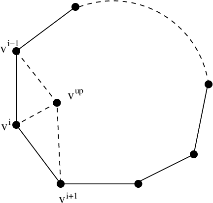
Since $c(v^{up})<c(v^{i})$, the complexity of this path is strictly smaller than that of the path $v^{1},\dots,v^{n}$. This proves Claim 2.

Now suppose that there is a homotopically nontrivial loop in the Kakimizu complex of $K$. By Theorem 3, there is a homotopically nontrivial loop $v^{1},\dots,v^{n}$ of smallest complexity. Then Claim 2 tells us that

$$c(v^{i})<max\{c(v^{i-1}),c(v^{i+1})\}\;\forall i.$$

But this is impossible. Thus the Kakimizu complex of $K$ is simply connected. ∎

We recall some of the standard terminology for simplicial complexes: The link of a vertex $v$ in a simplicial complex $X$, denoted by $X_{v}$, is the union of all simplices disjoint from $v$ that together with $v$ span a simplex in $X$. The star of a vertex $v$ in a simplicial complex $X$ is the union of all simplices in $X$ that contain $v$. A 2-dimensional simplicial complex $X$ is said to be locally $k$-large if for every vertex $v\in X$, every homotopically nontrivial loop in $X_{v}$ has length at least $k$.

The following theorem is classical. It follows from Propositions II.4.1 (Cartan-Hadamard Theorem) and II.5.25 in [4]. See Section 7 for a more general version.

$$d_{K}(v^{i+1},v^{down})\leq 1,d_{K}(v^{i-1},v^{down})\leq 1,d_{K}(v^{i+1},v^{up})\leq 1,d_{K}(v^{i-1},v^{up})\leq 1,$$

$$d_{K}(v^{i},v^{down})\leq 1,d_{K}(v^{i},v^{up})\leq 1,d_{K}(v,v^{down})\leq 1,d_{K}(v,v^{up})\leq 1$$

and (by part (b) of Lemma 2) also that

$$d_{K}(v^{i+2},v^{down})\leq 1,d_{K}(v^{i+2},v^{up})\leq 1.$$

Two cases need to be considered:

If $v^{down}$ is equal to one of the $v^{j}$, then the loop $v^{1},v^{2},v^{3},v^{4}$ breaks into two loops of length 3. The latter bound 2-simplices by Theorem 5. Hence we will assume that $v^{down}$ is not equal to one of the $v^{j}$. Now $v^{i-1},v^{i},v^{down}$ and $v^{i},v^{down},v^{i+1}$ are loops of length 3 and hence bound 2-simplices by Theorem 5. It follows that our loop

$$v^{i-1},v^{i},v^{i+1},v^{i+2}$$

is homotopic to

$$v^{i-1},v^{down},v^{i+1},v^{i+2}$$

in $X_{v}$. In addition, both $v^{down},v^{i+1},v^{i+2}$ and $v^{i+2},v^{i-1},v^{down}$ bound 2-simplices by Lemma 5. Thus $v^{i-1},v^{down},v^{i+1},v^{i+2}$ and hence $v^{i-1},v^{i},v^{i+1},v^{i+2}$, i.e., $v^{1},\dots,v^{4}$, is homotopically trivial in $X_{v}$. See Figure 5.

In this case we must argue differently. Let $F$ be a representative of $v$, $F_{0}$ a lift of $F$ to $M(K),$ $F_{1}=\tau(F_{0})$ and $C$ the component of

$$M(K)\backslash(F_{0}\cup F_{1})$$

that lies between $F_{0}$ and $F_{1}$. Recall the notation $S_{0}^{j},$ $\tilde{T}^{up},$ $\tilde{T}^{down},$ $S^{up},$ $S^{down}$ from the proof of Lemma 1 and let $\tilde{S}^{up},\tilde{S}^{down}$ be lifts of $S^{up},S^{down}$ to $C$, respectively. See Figure 6. We will assume (only) that $F,$ $F_{0},$ $F_{1}$ and each $S_{0}^{j}$ are least area surfaces in their isotopy classes.

References

- [1] C. Adams: The knot book. An elementary introduction to the theory of knots. American Mathematical Society, Providence, RI, 2004.
- [2] W. R. Alford: Complements of minimal spanning surfaces are not unique, Ann. Math. 91 (1970) 419–424.
- [3] M. Anderson: Curvature estimates for minimal surfaces in -manifolds, Ann. Sci. École Norm. Sup. (4), 18 (1985), pp. 89–105.
- [4] M. Bridson, A. Haefliger: Metric spaces of non-positive curvature. Grundlehren der Mathematischen Wissenschaften [Fundamental Principles of Mathematical Sciences], 319. Springer-Verlag, Berlin, 1999.
- [5] T. Colding, W. Minicozzi, II: Embedded minimal surfaces without area bounds in 3-manifolds, in Geometry and topology: Aarhus (1998), vol. 258 of Contemp. Math., Amer. Math. Soc., Providence, RI, 2000, pp. 107–120.
- [6] J. R. Eisner: Knots with infinitely many minimal spanning surfaces, Trans. Amer. Math. Soc. 229 (1977) 329–349.
- [7] M. Freedman, J. Hass, G. P. Scott: Area minimizing incompressible surfaces, Invent. Math. 71 (1983) 609–642.
- [8] J. Hass, P. Scott: The existence of least area surfaces in -manifolds, Trans. Amer. Math. Soc., 310 (1988), pp. 87–114.
- [9] M. Hirasawa, M. Sakuma: Minimal genus Seifert surfaces for alternating links, Proceedings of Knots 96 (1997) 383–394.
- [10] T. Januszkiewicz, J. Świa̧tkowski: Simplicial nonpositive curvature, Publications Mathématiques de l’Institut des Hautes Études Scientifiques, Volume 104, Number 1, November 2006, pp. 1-85.
- [11] O. Kakimizu: Finding disjoint incompressible spanning surfaces for a link, Hiroshima Math. J. 22 (1992) 225–236.
- [12] W.B.R. Lickorish: An introduction to knot theory. Graduate Texts in Mathematics 175. Springer-Verlag, New York, 1997.
- [13] N. Nakauchi: Compactness of incompressible stable minimal surfaces without boundary, J. of Mathematics of Kyoto University, 30 (1990), pp. 343–346.
- [14] U. Oertel: On the existence of infinitely many essential surfaces of bounded genus, Pacific J. Math. 202, no. 2 (2002) 449–458.
- [15] R. Pelayo: Diameter bounds on the complex of minimal genus Seifert surfaces for hyperbolic knots, thesis at California Institute of Technology, available at http://thesis.library.caltech.edu/2446/.
- [16] D. Rolfsen: Knots and links. Mathematics Lecture Series 7. Publish or Perish, Inc., Huston, TX, 1990.
- [17] M. Sakuma: Minimal genus Seifert surfaces for special arborescent links, Osaka J. Math. 31 (1994) 861–905.
- [18] M. Sakuma, K. Shackleton: On the distance between two Seifert surfaces of a knot, Osaka J. Math. 46 (2009) 203–221.
- [19] M. Scharlemann, A. Thompson: Finding disjoint Seifert surfaces, Bull. London Math. Soc. 20 (1988) 61–64.
- [20] R. Schoen: Estimates for stable minimal surfaces in three dimensional manifolds, in Seminar on minimal submanifolds, vol. 103 of Annals of Mathematics Studies, Princeton University Press, 1983, pp. 111–126.
- [21] K. Shackleton: private communication.
- [22] Y. Tsutsumi: Hyperbolic knots with a large number of disjoint minimal genus Seifert surfaces, Tokyo J. Math. 31 (2008), no. 1, 253–258.
- [23] R. Wilson: Knots with infinitely many incompressible Seifert surfaces, J. Knot Theory Ramifications 17 (2008), no. 5, 537–551.
Department of Mathematics
1 Shields Avenue
University of California, Davis
Davis, CA 95616