The phase structure of a chirally invariant lattice Higgs-Yukawa model -
numerical simulationsPreprint: HU-EP-07/28, DESY 07-108
Abstract
The phase diagram of a chirally invariant lattice Higgs-Yukawa model is explored by means of numerical simulations. The results revealing a rich phase structure are compared to analytical large calculations which we performed earlier. The analytical and numerical results are in excellent agreement at large values of . In the opposite case the large computation still gives a good qualitative description of the phase diagram. In particular we find numerical evidence for the predicted ferrimagnetic phase at intermediate values of the Yukawa coupling constant and for the symmetric phase at strong Yukawa couplings. Emphasis is put on the finite size effects which can hide the existence of the latter symmetric phase.
Keywords:
Higgs-Yukawa model, numerical simulation, hybrid Monte Carlo, phase diagramI Introduction
The main target of lattice studies of the Higgs-Yukawa sector of the electroweak standard model is the non-perturbative determination of lower and upper bounds of the Higgs boson mass Holland:2003jr; Holland:2004sd as well as its decay properties. There are two main developments which warrant to reconsider these questions: first, with the advent of the LHC, we are to expect that properties of the standard model Higgs boson, such as the mass and the decay width, will be revealed experimentally. Second, there is, in contrast to the situation of earlier investigations of lattice Higgs-Yukawa models, a consistent formulation of an exact lattice chiral symmetry Luscher:1998pq based on the Ginsparg-Wilson relation Ginsparg:1981bj.
Before questions of the Higgs mass bounds and decay properties can be addressed, the phase structure of the model needs to be investigated in order to determine the (bare) couplings in parameter space where eventual simulations of phenomenological interest can be performed. There has been a large activity of investigating lattice Higgs-Yukawa models in the past, see e.g. Refs. Smit:1989tz; Shigemitsu:1991tc; Golterman:1990nx; book:Montvay; book:Jersak; Golterman:1992ye; Jansen:1994ym for reviews. In particular, the phase structure of lattice Higgs-Yukawa models was investigated in great detail, see e.g. Refs. Hasenfratz:1989jr; Lee:1989mi; Bock:1990tv; Lin:1991cs; Hasenfratz:1991it; Hasenfratz:1992xs; Bock:1992yr; Bock:1997fu; Bock:1999qa for a still incomplete list. However, in these investigations, the lattice formulation of the corresponding Higgs-Yukawa theory broke explicitly chiral symmetry.
This situation changed when it was realized that the Ginsparg-Wilson relation Ginsparg:1981bj leads to the notion of an exact lattice chiral symmetry Luscher:1998pq allowing thus to go beyond the earlier models. Based on this development, the interest in lattice studies of Higgs-Yukawa models has been renewed Bhattacharya:2006dc; Giedt:2007qg; Poppitz:2007tu; KutiPrivateCom; Gerhold:2007yb. Here, we follow Lüscher’s proposition for a chirally invariant and hence consistent lattice Higgs-Yukawa model given in Ref. Luscher:1998pq. In particular, we want to address here the question whether the phase structure remains as complex as has been found out in the earlier work mentioned above. Additional and phenomenologically more interesting questions concerning the behaviour of the renormalized Higgs and Yukawa couplings will be addressed in future works.
In Gerhold:2007yb we have studied the phase structure of this chirally invariant Higgs-Yukawa model by means of a large computation, where denotes the number of fermion generations. We found a complex phase structure that resembles qualitatively the one of earlier lattice Higgs-Yukawa models, see e.g. Bock:1990tv, which, however, were lacking chiral symmetry. In the present paper we want to confront the results obtained in the large approximation with direct numerical simulations for finite values of . We remark that in the present work, as in Ref. Gerhold:2007yb, we neglect the gauge degrees of freedom and consider the pure scalar-fermion sector of the electroweak standard model.
To be more specific, we consider here a four-dimensional, chirally invariant Higgs-Yukawa model discretized on a finite lattice with lattice sites per dimension such that the total volume becomes . We set the lattice spacing to one throughout the paper. The model contains one four-component, real Higgs field and we consider fermion doublets represented by eight-component spinors , with . Furthermore, there are auxiliary fermionic doublets , serving as a construction tool in the creation of a chirally invariant Yukawa interaction term. Once the chiral invariance is established these unphysical fields are integrated out leading to a more complex model depending only on the Higgs field and the physical fermion doublets . The partition function is written as
| (1) |
with the total action being decomposed into the Higgs action , the kinetic fermion action , and the Yukawa coupling term . It should be stressed once again that no gauge fields are included within this model.
The kinetic fermion action describes the propagation of the physical fermion fields , in the usual manner according to
| (2) |
where the four-dimensional coordinates as well as all field variables and coupling constants are given in lattice units throughout this paper. The (doublet) Dirac operator is given by the Neuberger overlap operator , which is related to the Wilson operator by
| (3) |
with , denoting the forward and backward difference quotients. Note that in absence of gauge fields this kinetic part corresponds to the one of free fermions which will be exploited in the numerical construction of the overlap operator later. In particular, the eigenvalues of can be computed analytically. In momentum space with the allowed four-component momenta
| (4) |
the eigenvalues of the doublet operator are given by
| (5) |
We remark that the auxiliary fields do not propagate at all and that their contribution to is chosen such that the model will obey an exact lattice chiral symmetry.
The Higgs field couples to the fermions according to the Yukawa coupling term
| (6) |
where denotes the Yukawa coupling constant and will be referred to as Yukawa coupling matrix. Here the Higgs field is rewritten as a quaternionic, matrix , with denoting the vector of Pauli matrices, acting on the index of the fermionic doublets. Due to the chiral character of this model, left- and right-handed fermions couple differently to the Higgs field, as can be seen from the appearance of the projectors in the Yukawa term. Multiplying out the involved Gamma- and Pauli-matrices one can rewrite the coupling matrix in the compactified form
being block diagonal in position space. The model then obeys an exact, but lattice modified, chiral symmetry according to
| (10) | |||||
| (11) |
recovering the chiral symmetry in the continuum limit Luscher:1998pq.
Finally, the lattice Higgs action is given by the usual lattice notation
| (12) |
with the only particularity that the fermion generation number appears in the quartic coupling term which was a convenient convention for the large analysis. However, this version of the lattice Higgs action is equivalent to the usual continuum notation
| (13) |
with the bare mass and the bare quartic coupling constant . The connection is established through a rescaling of the Higgs field and the involved coupling constants according to
| (14) |
where denotes the Yukawa coupling constant corresponding to the continuum notation.
II Simulation Algorithm
The first step towards a numerical treatment of the considered Higgs-Yukawa model is to integrate out the fermionic degrees of freedom leading to the effective action
| (15) |
where the fermionic matrix
| (16) |
was given in Ref. Gerhold:2007yb.
Since we focus here on checking the validity of our earlier analytical investigation of the phase structure, which was determined in the large -limit, we will only consider even values for , allowing to rewrite the effective action according to
| (17) |
Thus the positivity of the determinant in Eq. (17) is guaranteed.
For the numerical treatment of the remaining determinant in Eq. (17) we have implemented an Hybrid-Monte-Carlo (HMC) algorithm Duane:1987de; Gottlieb:1987mq, with complex pseudo-fermionic fields according to the HMC-Hamiltonian
| (18) |
where denote the real momenta, conjugate to the Higgs field .
The application of the matrix on can then be performed by means of a Conjugate Gradient algorithm due to the hermiticity of . However, for the computation of , where is an arbitrary vector, we exploit the fact that there are no gauge fields included within our model. The eigenvectors of the used Neuberger overlap operator are therefore explicitly known to be the plane waves
| (19) |
with denoting the usual four-component spinor structure
| (20) |
Here are two orthonormal vectors and the four component quaternionic vector is defined as . The corresponding eigenvalues were given in Eq. (5). The operators and are thus both block-diagonal, the first in position space and the latter in momentum space. In our approach we use a Fast Fourier Transform (FFT) FFTW05 to switch between the position and momentum representations, such that all operator applications can be trivially performed due to their actual block-diagonal structure. This is particularly advantageous for the overlap operator, since the usual construction of this operator would be based on very demanding approximations, e.g. polynomial approximations.
A second advantage of this approach is that the applied Dirac operator can easily be replaced by other operators simply by adopting the corresponding eigenvalues.
Concerning the parallelization of the program there are several options. For example there are efficient parallelized FFT-routines available FFTW05. Here, however, we use a trivial - but very efficient - parallelization which is possible due to the large number of fermion generations . We simply perform each of the force calculations on a separate computer node.
For the integration of the obtained forces we find the Leap-Frog integration scheme to be efficient on small lattices. This situation changes with increasing lattice size and for we get better performance with higher order integrators. In that case we use an order 4 Omelyan-integrator Omelyan:2003; Takaishi:2005tz. The integration is then performed over a fixed trajectory length set to unity with the typical value for the step size. The step size is chosen such that the acceptance rate stays between and .
The observables we will be using for exploring the phase structure are the magnetization and the staggered magnetization ,
| (21) |
and the corresponding susceptibilities
| (22) |
where denotes the average over the -field configurations generated in the Monte-Carlo process.
The auto-correlation of our measurements of these observables in the Monte Carlo time is then accounted for by applying the -strategy Wolff:2003sm. In this approach the error of an observable is rewritten as a sum over the correlation function according to
| (23) |
where denotes the measurement of the observable in the -th configuration and is the total number of collected configurations. The variable is the window in which the function is to be summed up. It should be large enough to obtain reliable estimates of the auto-correlation time which is defined through the exponential decay rate of
| (24) |
and is thus directly connected to the sum of the auto-correlation function . Typical examples for the determination of by fitting the function to a constant are presented in Fig. 1. Since the auto-correlation length depends strongly on the distance to the phase transition we have selected one point in the parameter space close to the phase transition (Fig. 1a) and one point farer away from it (Fig. 1b). Both points correspond, however, to the ferromagnetic phase with a non-vanishing Higgs field expectation value, i.e. . For the Higgs field magnetization as the underlying observable we find in these examples the auto-correlation times in Fig. 1a and in Fig. 1b. We remark here that the value obtained in Fig. 1a is the largest auto-correlation time for the magnetization encountered in our studies. Although the auto-correlation time indeed increases when approaching the phase transition, its value remains acceptable for our purposes. Given that our typical statistics is -field configurations, this leads to reliable error determinations for the physical quantities of interest.
 |
 |
| (a) | (b) |
III Results for small values of the Yukawa coupling constant
In this section we will discuss the structure of the phase diagram at small values of the Yukawa coupling constant. All numerical results from our simulations are obtained by employing the algorithm as detailed in Section II. The anticipated structure of the phase diagram can be inferred from our large computation in Ref. Gerhold:2007yb. In that large approach the Higgs field and the coupling constants are scaled according to
| (25) |
where the quantities , , , and are held constant in the limit . Here, we want to confront this predicted phase structure with the results of our numerical simulations.
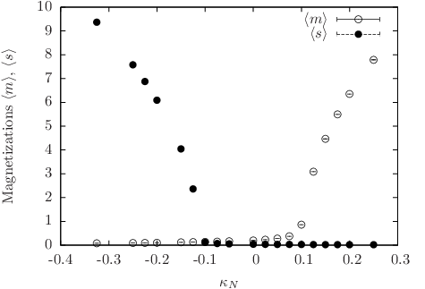
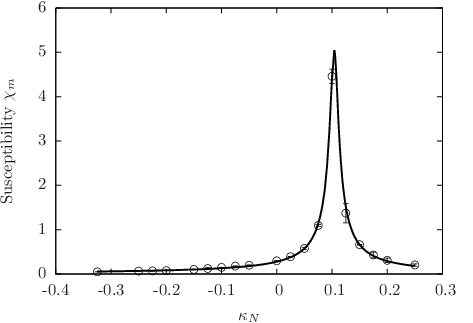
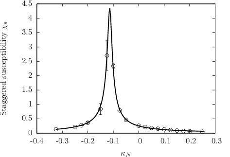
At small values of the Yukawa coupling constant, there are two phase transitions when varying : the first is a phase transition from a ferromagnetic (FM) phase, with and , to the symmetric (SYM) phase with . The second corresponds to a phase transition from the symmetric phase to an anti-ferromagnetic (AFM) phase with and . These phase transitions are expected to be of second order. To locate the phase transition points, we decided to fit the data for the susceptibilities , in Eq. (22) as a function of according to the – partly phenomenologically motivated – ansatz
| (26) |
where , , and are the fitting parameters for the magnetic susceptibility and staggered susceptibility, respectively, and , denote the critical exponents of the -theory. Here () is actually meant to refer to two parameters, namely () for () and () in the other case, such that the resulting curve is not necessarily symmetric. The phase transition point is then given at the value of () where the magnetic (staggered) susceptibility develops its maximum. We remark that the ansatz in Eq. (26), although not being unique, provides a very good description of our numerically obtained data leading to a reliable determination of the critical hopping parameters .
 |
 |
 |
| (a) | (b) | (c) |
In Fig. 2 we present a typical example for the determination of the phase transition points at small values of the Yukawa coupling constant. The average magnetizations and as well as the corresponding susceptibilities are shown as a function of . We clearly observe the vanishing of the magnetization and the staggered magnetization when the symmetric phase is entered (except for some small finite volume effects). Associated with these transitions are peaks in the susceptibilities. Note that the data for the susceptibilities are fitted very well using the ansatz of Eq. (26), allowing for a good determination of the critical points.

Using the strategy just described we computed the values of and for various Yukawa coupling constants holding the quartic coupling constant. In Fig. 3 we summarize the numerical results for the phase structure as obtained on - and -lattices at and compare them to the analytical , phase structure. As expected we observe a symmetric (SYM), a ferromagnetic (FM) and an anti-ferromagnetic (AFM) phase, with the symmetric phase bending strongly towards smaller values of the critical hopping parameter when the Yukawa coupling constant is increased.
As a general remark we note here that the simulations become extremely demanding when entering the anti-ferromagnetic phase, due to an increasingly bad condition number of the fermionic matrix . Within the anti-ferromagnetic phase we thus only present numerical results obtained on -lattices throughout this paper.
 |
 |
| (a) | (b) |
Besides these three phases also a fourth, somewhat peculiar phase that can appear at intermediate values of the Yukawa coupling constant was predicted by our analytical investigation. This is the so-called ferrimagnetic (FI) phase where both, the average magnetization as well as the average staggered magnetization, are non-zero, i.e. and . It was found that such a ferrimagnetic phase should exist deeply inside the anti-ferromagnetic phase Gerhold:2007yb. In Fig. 4 we provide evidence for the existence of this ferrimagnetic phase. Its location within the phase diagram is in good agreement with the analytical prediction. However, the ferrimagnetic phase is not the prime target for our eventual interest and hence we do not further investigate this phase here.
Concerning the order of the encountered phase transitions we find that the SYM-FM as well as the SYM-AFM phase transition seem to be of second order in accordance with the continuous behaviour of and as seen e.g. in Fig. 4a. This is in contrast to the direct FM-AFM phase transition that should occur at intermediate values of the Yukawa coupling constant according to our large computation. From the analytical considerations we expect this transition to be of first order. To clarify this we show in Fig. 5 an example for such a phase transition as seen in the numerical simulations. One can clearly observe an abrupt jump in and in Fig. 5a indicating a discontinuous phase transition. In subfigures (b) and (c) we furthermore present an example for a tunneling event between two ground states close to the critical value of the hopping parameter serving as another strong indication for the first order nature of the phase transition at intermediate values of the Yukawa coupling constant. However, we do not study the order of the phase transition in great detail here, since this is not in our main interest.
 |
 |
 |
| (a) | (b) | (c) |
Qualitatively, all presented findings are in excellent accordance with our large calculations in Ref. Gerhold:2007yb. On a quantitative level, however, the encountered deviations in Fig. 3 need to be further addressed. These deviations can be ascribed to finite volume effects as well as finite corrections. Here we start with a discussion of the finite volume effects.
The location of the phase transition points can be strongly altered by finite size effects. This is illustrated in Fig. 6 showing some phase transition points from the FM to the SYM phase as obtained from our numerical simulations on a -lattice (open squares), and on an -lattice (open circles). One clearly observes that the phase transition line is shifted towards smaller values of the hopping parameter when the lattice size is increased. This effect can also be anticipated from the analytical computation of the phase transition line, when one imposes finite lattices also for the minimization of the effective potential in the large approximation. Since we want to demonstrate the finite volume dependence here isolated from the -dependence, we present the numerical results for the (very large) value of fermion generations and compare them to the analytical phase transition lines obtained for (dotted line), (dashed line), and (solid line). The analytical lines perfectly describe the numerical results and one clearly observes the convergence of the numerical results to the analytically predicted line as the lattice size increases.
However, one remark is in order here for the orientation of the reader, which concerns the large -computation of the phase transition points in a finite volume: The fermionic determinant with given in Eq. (16) becomes, on a finite lattice, identical to zero for completely vanishing Higgs field. On infinite lattices the zero modes of form a set of only zero measure and the integral entering the effective action can be shown to converge, such that there actually is a symmetric phase on infinite lattices. For finite we therefore cannot determine the phase transition by simply searching that value of the hopping parameter, where the average magnetization vanishes. Instead we search for that , where the minimum of the effective action becomes flattest, i.e. where the second derivative of with respect to the magnetization becomes minimal at the location of the minimum. Since the Higgs field oscillates the stronger around the minimum of the effective action the smaller its second derivative is, this approach corresponds to finding the phase transition point by searching for the maximum of the susceptibility.

The -dependence of the numerically obtained critical hopping parameters and is shown in Fig. 7 for several selected values of the Yukawa coupling constant. One clearly sees that for increasing the numerical results converge very well to the analytical finite volume predictions, as expected. It is interesting to note that the leading term in the finite corrections, i.e. the contribution, seems to be the only relevant correction here, even at the small value , as can be seen in Fig. 7 by fitting the deviations to the function with being the only free parameter. Furthermore, one observes that the critical hopping parameter is shifted towards larger values with decreasing while is shifted towards smaller values.
 |
 |
 |
| (a) | (b) | (c) |
From our findings in this section we finally conclude that the structure of the phase diagram of the considered Higgs-Yukawa model at small values of the Yukawa coupling constant can be very well predicted on a qualitative level by the results of our large analysis. It also gives a very good understanding of the encountered finite volume effects.
IV Results for large Yukawa coupling constant
In this section we want to address the region of large Yukawa coupling constants, i.e. . From our large calculations we expect here a ferromagnetic, an anti-ferromagnetic and a symmetric phase. The large calculation also revealed that significant finite size effects can be present in the symmetric phase which may render its detection difficult. This large approach was carried out by scaling the Higgs field and the coupling constants according to
| (27) |
where the quantities , , , and were held constant in the limit .
 |
 |
 |
| (a) | (b) | (c) |
In Fig. 8, we show the numerically obtained values for the average magnetizations and on various sized lattices as a function of for a large value of the Yukawa coupling constant . Fig. 8 demonstrates that indeed the symmetric phase emerges only on sufficiently large lattices, while on small lattices the magnetization does not vanish as a function of decreasing even deeply within the anti-ferromagnetic phase. Instead reaches a plateau with a clearly non-vanishing value in the limit . This becomes especially well observable for the smallest considered lattice, the -lattice presented in Fig. 8a. Thus, one may erroneously conclude that there is no symmetric phase at large values of the Yukawa coupling constant, if one considers too small lattices. However, the plateau value of is fully consistent with our analytical results predicting a finite volume effect causing a non-vanishing magnetization also for arbitrarily negative values of . To demonstrate this latter statement we restate here one result of Ref. Gerhold:2007yb for the effective action of a field configuration in terms of its magnetizations and in the large -limit, reading
| (28) |
with the abbreviations
| (29) |
Considering only the ground state of this effective action one cannot correctly predict the phase transition of the model, as discussed in Ref. Gerhold:2007yb. However, it is sufficient to correctly predict the behaviour of and in the limit of large negative (and positive) values of the hopping parameter , as demonstrated in Fig. 9, where we plot again the average magnetizations for the -lattice together with the finite volume analytical expectations, obtained by minimizing the effective action of Eq. (28). The convergence of the numerical results to the analytical finite volume prediction is very well observed in Fig. 9b.
 |
 |
| (a) | (b) |
We remark that the non-vanishing plateau as well as the asymmetry in and are both caused by the term appearing in Eq. (28). This term as well as the very last one in this equation do, however, not scale proportional to the volume in contrast to all other contributions to the effective action. Its influence therefore eventually disappears as the lattice size increases. This is exactly what is observed here.
 |
 |
 |
| (a) | (b) | (c) |
In Fig. 10 we show the susceptibilities corresponding to the magnetizations in Fig. 8. For the smallest lattice, i.e. the -lattice, one observes only one peak in the magnetic susceptibility, centered at . From this result one could conclude that the phase transition point is located at , excluding a symmetric phase, since the staggered susceptibility reaches its maximum at the same value of . However, with increasing lattice sizes a second peak develops in the susceptibilities. This is very well observed in Fig. 9b corresponding to the larger -lattice. It shows that indeed two distinct peaks emerge on this intermediate lattice. It is actually this second peak, centered around in this case, that correctly describes the physical phase transition between the ferromagnetic and the symmetric phase, while the first one is only caused by the finite volume terms discussed in Gerhold:2007yb, which do not scale with the lattice volume. Its height is therefore at most constant in contrast to the physical peak, which grows with increasing lattice volume. On the largest presented lattice, the -lattice, the physical peak at completely dominates the scene and the former small volume peak at has disappeared, presumably hidden beneath the large error bars at .

We have then determined the SYM-FM phase transition points by fitting the physical peaks in the magnetic susceptibility on the intermediate -lattices to the finite volume expectation in Eq. (26) by taking only the points belonging to the physical peak into account as demonstrated in Fig. 10b. We remark here that we do not provide any data for the SYM-AFM phase transition because the phase transition is not reliably detectable on the -lattice, due to the finite volume effects discussed above, and the -simulations are not practicable in the anti-ferromagnetic phase with our algorithm as explained in Section III.
In Fig. 11 we finally summarize the obtained phase transition points together with the analytical , expectation of the phase structure at large values of the Yukawa coupling constant. Qualitatively, the picture we obtain from the numerical simulations is in full accordance with the results from the large approximation: there are second order phase transitions separating a ferromagnetic phase from a symmetric phase. In this symmetric phase strong finite size effects are encountered such that only for large lattice sizes this symmetric phase can be identified. Quantitatively, the numerical results deviate from the analytical expectation due to the finite settings and , but are still in good agreement.
In this section we found that a symmetric phase at large values of the Yukawa coupling constant does indeed exist although its existence is obscured on too small lattices by strong finite size effects, and that its location within the phase diagram is in good agreement with the analytical large predictions. We remark here that the existence of a symmetric phase at strong Yukawa couplings has also been observed and discussed in Ref. Giedt:2007qg. From our findings we thus conclude that the analytical large calculations describe the phase structure of the considered Higgs-Yukawa model at large values of the Yukawa coupling constant very well.
V Summary and outlook
In this paper we have studied by numerical simulations the phase structure of a chirally invariant lattice Higgs-Yukawa model, originally proposed by Lüscher, in order to check the validity of our earlier analytical investigation of its phase structure. These earlier calculations have been performed in the large -limit for small and for large values of the Yukawa coupling constant.
In Section III we compared the numerical to the analytical results at small values of the Yukawa coupling constant. We started with a discussion of the qualitative structure of the phase diagram. For that purpose we presented our numerical results for the phase transition lines obtained at on some - and -lattices and compared them to the analytically computed , predictions. Qualitatively, the numerical and analytical results are in very good agreement: As expected we clearly observe a symmetric (SYM), a ferromagnetic (FM) and an anti-ferromagnetic (AFM) phase. With increasing Yukawa coupling constant the symmetric phase strongly bends downwards to smaller values of the hopping parameter. In particular, we find that the obtained phase structure resembles that of earlier Higgs-Yukawa models on a qualitative level. One peculiarity in these types of models is the emergence of a ferrimagnetic (FI) phase with and deeply inside the anti-ferromagnetic phase. This phase was also predicted by the analytical investigation of the model and it is located at the predicted position within the phase diagram. Furthermore, the data also support very well the analytical expectations concerning the order of the encountered phase transitions. The SYM-FM and the SYM-AFM phase transitions were supposed to be of second order while the direct FM-AFM transition was predicted to be of first order. Although we did not study that in great detail, since this aspect was not in out main interest, the obtained lattice results are in very good agreement with these analytical findings.
We then turned towards the quantitative discussion of the encountered deviations between the numerical finite volume, finite results and the presented analytical , calculations. Firstly, we showed that finite volume effects alter the location of the phase transition lines strongly. In order to isolate the finite volume effects from the corrections we presented numerical results for the phase transition points for the choice of the very large number of fermion generations . In that setting we could show that the finite volume effects are in excellent agreement with the analytical finite volume predictions. We then demonstrated the strength of the corrections by presenting the numerically obtained phase transition points at smaller values of for some selected Yukawa coupling parameters. We found that the corrections drive the critical hopping parameters towards larger values for the case of the SYM-FM phase transition and towards smaller values for the SYM-AFM transition. Besides that these corrections do not change the qualitative phase structure of the model.
We then discussed the phase structure at large values of the Yukawa coupling constant in Section IV. In particular we showed that there is actually a symmetric phase in this regime of the Yukawa coupling constant and that it is located at the expected position within the phase diagram. We also demonstrated that this symmetric phase becomes unobservable on too small lattices due to strong finite volume effects, as derived in our earlier studies, preventing the Higgs field expectation value from vanishing. We furthermore showed that the behaviour of the magnetization at large negative (and positive) values of the hopping parameter can be very well described by taking these finite volume contributions into account. The emergence of the symmetric phase with increasing lattice size could also clearly be observed in the presented plots of the magnetic susceptibility (Fig. 10). Finally, we presented our numerical results for the critical hopping parameters of the SYM-FM phase transition at large Yukawa coupling constants. We compared them to the analytical large predictions and found them to be in good agreement even though the numerical simulations were performed at .
We end with a short outlook about our next steps concerning the further investigation of the presented Higgs-Yukawa model: We have started the implementation of a PHMC algorithm Frezzotti:1998eu with which the simulation will become possible at arbitrary values of , in particular at the physically interesting setting . Having the qualitative phase diagram of the model at hand we will then search for the physical region of the parameter space, reproducing the top quark mass, eventually allowing to find upper and lower bounds for the Higgs boson mass.
Acknowledgments
We thank the ”Deutsche Telekom Stiftung” for supporting this study by providing a Ph.D. scholarship for P.G. We further acknowledge the support of the DFG through the DFG-project Mu932/4-1. We are grateful to Joel Giedt, Julius Kuti, Michael Müller-Preussker, Erich Poppitz, and Christopher Schroeder for enlightening discussions and comments. In particular we want to express our gratitude to Julius Kuti for inviting P.G. to his group at the University of California, San Diego.
References
- (1) K. Holland and J. Kuti. How light can the Higgs be. Nucl. Phys. Proc. Suppl. 129:765–767, 2004.
- (2) K. Holland. Triviality and the Higgs mass lower bound. Nucl. Phys. Proc. Suppl. 140:155–161, 2005.
- (3) M. Lüscher. Exact chiral symmetry on the lattice and the Ginsparg- Wilson relation. Phys. Lett. B428:342–345, 1998.
- (4) P. H. Ginsparg and K. G. Wilson. A remnant of chiral symmetry on the lattice. Phys. Rev. D25:2649, 1982.
- (5) J. Smit. Standard model and chiral gauge theories on the lattice. Nucl. Phys. Proc. Suppl. 17:3–16, 1990.
- (6) J. Shigemitsu. Higgs-Yukawa chiral models. Nucl. Phys. Proc. Suppl. 20:515–527, 1991.
- (7) M. F. L. Golterman. Lattice chiral gauge theories: Results and problems. Nucl. Phys. Proc. Suppl. 20:528–541, 1991.
- (8) I. Montvay and G. Münster. Quantum Fields on a Lattice (Cambridge Monographs on Mathematical Physics). Cambridge University Press, 1997.
- (9) A. K. De and J. Jersák. Yukawa models on the lattice. HLRZ Jülich, HLRZ 91-83, preprint edition, 1991.
- (10) M. F. L. Golterman, D. N. Petcher, and E. Rivas. On the Eichten-Preskill proposal for lattice chiral gauge theories. Nucl. Phys. Proc. Suppl. 29BC:193–199, 1992.
- (11) K. Jansen. Domain wall fermions and chiral gauge theories. Phys. Rept. 273:1–54, 1996.
- (12) A. Hasenfratz, W. Liu, and T. Neuhaus. Phase structure and critical points in a scalar fermion model. Phys. Lett. B236:339, 1990.
- (13) I.-H. Lee, J. Shigemitsu, and R. E. Shrock. Study of different lattice formulations of a Yukawa model with a real scalar field. Nucl. Phys. B334:265, 1990.
- (14) W. Bock et al. Phase diagram of a lattice SU(2) x SU(2) scalar fermion model with naive and Wilson fermions. Nucl. Phys. B344:207–237, 1990.
- (15) L. Lin, I. Montvay, and H. Wittig. Phase structure of a U(1)-L x U(1)-R symmetric Yukawa model. Phys. Lett. B264:407–414, 1991.
- (16) A. Hasenfratz, P. Hasenfratz, K. Jansen, J. Kuti, and Y. Shen. The Equivalence of the top quark condensate and the elementary Higgs field. Nucl. Phys. B365:79–97, 1991.
- (17) A. Hasenfratz, K. Jansen, and Y. Shen. The Phase diagram of a (1) Higgs-Yukawa model at finite lambda. Nucl. Phys. B394:527–540, 1993.
- (18) W. Bock, J. Smit, and J. C. Vink. Fermion Higgs model with reduced staggered fermions. Phys. Lett. B291:297–305, 1992.
- (19) W. Bock, M. F. L. Golterman, and Y. Shamir. On the phase diagram of a lattice U(1) gauge theory with gauge fixing. Phys. Rev. D58:054506, 1998.
- (20) W. Bock, K. C. Leung, M. F. L. Golterman, and Y. Shamir. The phase diagram and spectrum of gauge-fixed Abelian lattice gauge theory. Phys. Rev. D62:034507, 2000.
- (21) T. Bhattacharya, M. R. Martin, and E. Poppitz. Chiral lattice gauge theories from warped domain walls and Ginsparg-Wilson fermions. Phys. Rev. D74:085028, 2006.
- (22) J. Giedt and E. Poppitz. Chiral lattice gauge theories and the strong coupling dynamics of a Yukawa-Higgs model with Ginsparg-Wilson fermions. arXiv: hep-lat/0701004, 2007.
- (23) E. Poppitz and Y. Shang. Lattice chirality and the decoupling of mirror fermions. arXiv: 0706.1043 [hep-th], 2007.
- (24) J. Kuti and C. Schroeder. Private communication. 2007.
- (25) P. Gerhold and K. Jansen. The phase structure of a chirally invariant lattice Higgs-Yukawa model for small and for large values of the Yukawa coupling constant. arXiv: 0705.2539 [hep-lat], 2007.
- (26) S. Duane, A. D. Kennedy, B. J. Pendleton, and D. Roweth. Hybrid Monte Carlo. Phys. Lett. B195:216–222, 1987.
- (27) S. A. Gottlieb, W. Liu, D. Toussaint, R. L. Renken, and R. L. Sugar. Hybrid Molecular Dynamics Algorithms for the Numerical Simulation of Quantum Chromodynamics. Phys. Rev. D35:2531–2542, 1987.
- (28) M. Frigo and S. G. Johnson. The design and implementation of FFTW3. Proceedings of the IEEE 93(2):216–231, 2005. special issue on ”Program Generation, Optimization, and Platform Adaptation”.
- (29) I. P. Omelyan, I. M. Mryglod, and R. Folk. Comput. Phys. Commun. 151:272, 2003.
- (30) T. Takaishi and P. de Forcrand. Testing and tuning new symplectic integrators for hybrid Monte Carlo algorithm in lattice QCD. Phys. Rev. E73:036706, 2006.
- (31) U. Wolff. Monte Carlo errors with less errors. Comput. Phys. Commun. 156:143–153, 2004.
- (32) R. Frezzotti and K. Jansen. The PHMC algorithm for simulations of dynamical fermions. I: Description and properties. Nucl. Phys. B555:395–431, 1999.