Nucleon Structure and Hyperon Form Factors from Lattice QCDPreprint: JLAB-THY-07-687
Abstract
In this work, I report the latest lattice QCD calculations of nucleon and hyperon structure from chiral fermions in 2+1-flavor dynamical simulations. All calculations are done with a chirally symmetric fermion action, domain-wall fermions, for valence quarks. I begin with the latest lattice results on the nucleon structure, focusing on results from RBC/UKQCD using 2+1-flavor chiral fermion actions. We find the chiral-extrapolated axial coupling constant at physical pion mass point to be 1.23(5), consistent with experimental value. The renormalization constants for the structure functions are obtained from RI/MOM-scheme non-perturbative renormalization. We find first moments of the polarized and unpolarized nucleon structure functions at zero transfer momentum to be 0.133(13) and 0.203(23) respectively, using continuum chiral extrapolation. These are consistent with the experimental values, unlike previous calculations which have been 50% larger. We also have a prediction for the transversity, which we find to be 0.56(4). The twist-3 matrix element is consistent with zero which agrees with the prediction of the Wandzura-Wilczek relation.
In the second half of this work, I report an indirect dynamical estimation of the strangeness proton magnetic moments using mixed actions. With the analysis of hyperon form factors and using charge symmetry, the strangeness of proton is found to be , consistent with the Adelaide-JLab Collaboration’s result. The hyperon and axial coupling constants are also performed for the first time in a lattice calculation, and .
pacs
11.15.Ha,12.38.Gc,12.38.Lg,14.40.-nI Introduction
Quantum chromodynamics (QCD) has been successful in describing many properties of the strong interaction. In the weak-coupling regime, we can rely on perturbation theory to work out the path integral which describes physical observables of interest. However, for long distances perturbative QCD no longer converges. Lattice QCD allows us to calculate these quantities from first principles.
In Lattice QCD, space and time are discretized in a finite volume, and we use Monte Carlo integration to evaluate the remaining integral. Since the real world is continuous and infinitely large, at the end of the day we will have to take and . However, using current computer resources, we cannot yet simulate full QCD at the physical pion mass. With the help of the chiral perturbation theory and calculations at multiple heavier pion masses which are affordable in terms of available computational resources, we can extrapolate quantities of interest to the physical limit. Such calculations also help to determine the low-energy constants of the chiral effective theory.
There are a few choices of fermion action that have been commonly used in lattice QCD calculations. Each has its own pros and cons. They differ primarily by how they maintain symmetry, their calculation cost and their discretization error. The consistency of results from different fermion actions demonstrates the university of discretizations from lattice QCD.
The most expensive class of discretization are the chiral fermion actionsKaplan 1992; Kaplan 1993; Shamir 1993; Furman and Shamir 1995: domain-wall fermion (DWF) or overlap fermion. Such actions maintain the chiral symmetry of the fermions at great cost, but for this cost, we derive significant benefits. The theory is automatically improved which makes it particularly well suited for spin physics and weak matrix elements. Since symmetry remains at the non-zero lattice spacing, it further simplifies the renormalization calculation on the lattice and the chiral extrapolation.
A much cheaper alternative is the (improved) staggered fermion action (asqtad)Kogut and Susskind 1975; Orginos and Toussaint 1999; Orginos et al. 1999. The relatively fast simulation has great potential to be the first lattice calculation to reach the physical pion mass with 2+1 flavors. However, it introduces the problem of taste: each single fermion in the action contains four tastes. Although these extra tastes can be removed by the “root trick”, mixing among different parities and tastes remains in the theory. There have been spirited debates over whether it is proper to use asqtadCreutz 2006; Sharpe 2006, but for practical purposes no evidence of anomalous results have yet been found; theoretical proof of its correctness is an ongoing effort. However, the issue of taste-breaking makes baryonic operators a nightmare to work with, regardless of any potential cost savings.
One might combine the best features of both of these actions by using a mixed action. Cheap staggered fermions can be used for the expensive sea quarks, while chiral domain-wall fermions are used in the valence sector, where they protect operators from mixing. We will discuss the employment of such an action in the final section.
In this work, we use lattice QCD techniques to pursue long-distance physics, solving non-perturbative QCD from first principles. The structure of this article is as follows: In Sec. II, I report the latest 2+1f DWF valence calculation using RBC/UKQCD gauge configurations. In this work, we concentrate on the results for the axial coupling constant, first moment of the unpolarized quark and helicity distributions, and the zeroth moment of the transversity and twist-3 matrix element . We reproduce the experimental numbers for the first three quantities using continuum perturbation theory, predict the value of the transversity at leading order and check the Wandzura-Wilczek relation. We also compare our results with those of other lattice groups. In the Sec. III, I present some work done by the Jefferson Lab hyperon project, calculating the proton strange magnetic moment and the axial couplings of the hyperons. This is the first time that the strange magnetic moment is done using dynamical lattice data, and we find a value consistent with the Adelaide-JLab Collaboration’s result. The and axial coupling is for the first time done in lattice QCD. We find the numbers are more accurate than what had been estimated by the chiral perturbation theory or large- theory.
II Nucleon Structure
II.1 Lattice Parameters
In this calculation, we uses lattices generated by the RBC/UKQCD collaborations with the chiral DWF action and a full 2+1-flavor dynamical quark sector. The ensembles range in pion mass from 625 down to 300 MeV, at a lattice scale 1.6 GeV in a 3 fm box. The details of the gauge configurations can be found in Ref. Allton et al. 2007 for hadron properties in a 2 fm box.
On these ensembles, we use a Gaussian-smeared source to improve the signals. The source-sink separation is fixed at 12 time units. The choices of sink and the corresponding number of configurations in this work are listed in Table 1.
| 0.005 | 0.01 | 0.02 | 0.03 | |
|---|---|---|---|---|
| # of conf. | 180 | |||
| (GeV) | 0.319(3) | 0.399(3) | 0.535(3) | 0.625(3) |
| (GeV) | 1.085(16) | 1.169(19) | 1.204(13) | 1.474(18) |
The interpolating field used in our calculation is
| (1) |
We calculate the nucleon two-point function ( of with smearing parameters and ) as
| (2) |
and three-point function which is defined as
| (3) |
where is the operator of interest. For more details, please refer to our earlier work in Refs. Lin et al. 2007; Orginos et al. 2006; Sasaki et al. 2003.
When one calculates the three-point Green function, there are two possible contraction topologies: “connected” and “disconnected” diagrams, as depicted in Figure 1. Disconnected pieces are notoriously difficult to calculate directly on the latticeMathur and Dong 2001; Dong et al. 1998; Lewis et al. 2003; Foley et al. 2005. It would require numerous source vectors in the fermion-matrix inversion, and there was no reasonable way of calculating these contributions when this calculations started. However, this difficulty might be resolved in the near future with development of new techniques by members of the USQCD collaboration. In this work, only “isovector” quantities will be discussed, in which the disconnected piece cancels under isospin symmetry.


We apply nonperturbative renormalization (NPR) in RI/MOM schemeMartinelli et al. 1995 to the above quantities. In general, the operators of interest can mix with lower-dimension operators as
| (4) |
With the good chiral symmetry of DWF action, however, we are protected from this mixing problem. We calculate in RI/MOM scheme, where must fall inside the renormalization window . Then we convert to scheme Gimenez et al. 1998, running to 2 GeV to get the renormalization constant for the operators. In this work, the NPR is done on a smaller lattice ensemble, the 2 fm ones; since it is a short-distance quantity, the renormalization constants are not as sensitive to finite-volume effects as other observables. Detailed step-by-step descriptions can be found in Refs. Lin et al. 2007; Orginos et al. 2006. The renormalization constant in RI/MOM and scheme for first moment of the unpolarized distribution and helicity and zeroth moment of the transversity (from top to bottom) are shown in the Figure 2.


II.2 Numerical Results
II.2.1 Axial Coupling Constant
The axial charge is well measured in the neutron decay experiment and hence it is a natural candidate to demonstrate how well the lattice QCD approach with the chiral extrapolation to the physical pion point. The isovector vector and axial charges, and , are defined as the zero-momentum-transfer limits of the following,
| (5) | |||||
| (6) |
Because of chiral symmetry on our fermion action, a Takahashi-Ward identity ensures that the two currents, which are related by chiral transformation, share a common renormalization: up to a lattice discretization error of . Since the vector current is conserved, its renormalization is easily obtained as the inverse of the vector charge . Thus, by calculating the ratio of the three-point functions for , we get the renormalized axial charge, . The results are shown as red triangles in Figure 3.
In order to reach the physical pion mass value for our result, we adopt the chiral extrapolation expression from the the small-scale expansion (SSE) schemeHemmert et al. 1998. In this scheme, one uses explicit degrees of freedom from the pion, nucleon and , then expands in terms of , the mass splitting between the and in the chiral limit, which is treated as . Here we adopt a formulation which is correct up to , as seen in Ref. Hemmert and Weise 2002; Hemmert et al. 2003, and we also try its finite-volume corrected form. The grey band in Figure 3 indicates the uncertainty due to the jackknife chiral extrapolation with SSE formulation; our preliminary extrapolated axial coupling constant is 1.23(5), consistent with experimental data. If we add finite-volume effects, with the lattice box fixed at 3 fm, we can see the correction at our pion mass points are tiny, as indicated by the green band. In right of Figure 3, we compare our result to that of other lattice groupsEdwards et al. 2006; Gockeler et al. 2006; Khan et al. 2006; Khan et al. 2004; Dolgov et al. 2002 and to our previous calculation Lin et al. 2007; Sasaki et al. 2003. Compared with our previous DWF quenched 2.4 fm and 2-flavor 2 fm box calculations, we see a clear consistency in the axial charge coupling. In fact, most of the calculations (either using chiral fermion or not) are consistent with each other. One thing to notice is that we currently have the lightest dynamical pion mass point, although the result from the lightest ensemble (in both our 2- and 2+1-flavor) deviates from the chiral extrapolation curve. We have more gauge ensembles in the 2+1-flavor case, and we will be able to verify in the near future whether this is just simply due a lack of statistics or to a finite-volume effect that is not accounted accurately by the chiral perturbation theory.


(right) The axial charge comparison from various lattice group
II.2.2 Unpolarized quark and helicity distribution
The moments of the unpolarized quark distribution and helicity distribution are defined as:
| (7) | |||||
| (8) |
where is the sum of the quarks with helicity aligned and anti-aligned () and is the difference of the two ( ). On the lattice, this corresponds to the matrix elements of the operators
| (9) | |||||
| (10) |
respectively with the difference between the covariant derivatives. Note that here the trace term which corresponds to the disconnected piece is not included in our calculation. Therefore, we will look at the difference between the up and down quark contribution where this contribution is negligible.
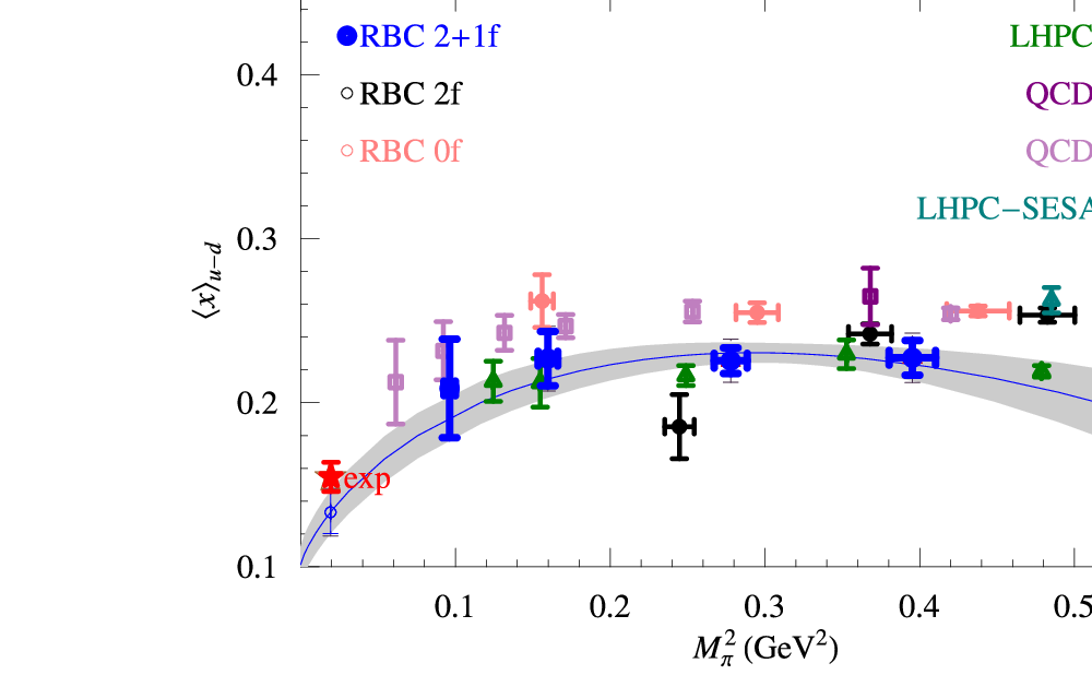
In this work, we will only concentrate on the first moments of the unpolarized and helicity distributions, and respectively. The corresponding renormalization constants are obtained using RI/MOM-scheme NPR as described in Sec. II.1. The renormalized moments are shown in Figure 4 at each pion mass point. Again, we use help from chiral effective theoryDetmold et al. 2001; Arndt and Savage 2002; Chen and Savage 2002; Detmold et al. 2002 for these quantities to extrapolate to the physical pion point:
| (11) | |||||
| (12) |
This chiral behavior is indicated in the blue line in Figure 4. We see a strong curvature due to the chiral form; more light-pion points should be taken to eliminate extrapolation uncertainties. In the past, we have been finding these quantities to be about 50% larger than the experimental ones. (See Ref. Lin et al. 2007; Orginos et al. 2006 for example.) In this updated 2+1f DWF calculation, these moments are 0.133(13) and 0.203(23). Figure 5 shows a list of the latest calculations of the first moments of the unpolarized (left) and helicity (right) distributions. Here we can see the quenched or partially quenched approximation results either from our past DWF calculation Lin et al. 2007; Orginos et al. 2006 or from the QCDSF/LHPCDolgov et al. 2002; Orginos 2006. Our preliminary results seem to be consistent with the LHPC’s mixed action calculationEdwards et al. 2006, although more statistics in the near future will help us to clarify what role the staggered sea plays in these quantities.



II.2.3 Transversity
Another interesting quantity regarding the spin structure of nucleon is transversity. The moments of transversity are defined as
| (13) |
where is the difference between the quarks with spin aligned and anti-aligned with the polarized target. On the lattice, this corresponds to the matrix elements of the operator
| (14) |
Again, we only calculate the isovector quantity to eliminate the contribution from the disconnected diagrams.
We calculate the zeroth moment of transversity, , and the results are given on the left-hand side of Figure 6. We observe rather weak dependence (linear extrapolation) on the quark mass. We use the chiral extrapolation formulationDetmold et al. 2001; Arndt and Savage 2002; Chen and Savage 2002; Detmold et al. 2002
| (15) |
and get 0.56(4) at physical pion mass point. This extrapolated value is significant smaller than the simulated pion mass point, which is of order 1 or so. We urgently need data from our lightest pion mass to confirm this rapid decreasing behavior. However, this is close to what has been found by LHPC with mixed actionEdwards et al. 2006, about 0.7; their data is listed on the right-hand side of Figure 6. Their results at each pion mass are consistent within our current statistics. Apparently, the total suppression of sea quarks plays an important roles, as seen in comparing our quenched and dynamical numbers; however, there is not much difference between 2 and 2+1 flavors.


II.2.4
The twist-3 first moment of the polarized structure function is another interesting feature to consider. It is related to the polarized structure functions and by the operator
| (16) |
It mixes with the lower-dimensional operator if the lattice fermions do not have chiral symmetry at finite lattice spacing; we are free of this problem in our calculation. Although it is not measurable in deep inelastic scattering of electrons on protons, it gives us some expectation of the higher moment matrix elements. Figure 7 shows our isovector matrix element results. We extrapolate the twist-3 matrix element to the physical pion mass and get , which is consistent with zero. Combined with the small value of from QCDSFGockeler et al. 2001, we conclude that the Wandzura-Wilczek relation between moments of and Wandzura and Wilczek 1977, which asserts vanishing , is at least approximately true.

III Hyperons
III.1 Lattice Parameters
We use a mixed action, meaning that the sea and valence fermions use different discretizations. In our case, the sea fermions are 2+1 flavors of staggered fermions (in configuration ensembles generated by the MILC collaborationBernard et al. 2001), and the valence fermions are domain-wall fermions. The pion mass ranges from 360 to 700 MeV in a lattice box of size 2.6 fm. The strange-strange Goldstone is fixed at 763(2) MeV, which unfortunately does not reproduce the physical strange-strange Goldstone mass. The gauge fields are hypercubic-smeared to improve the chiral symmetry of the fermion, and the fermion field is Gaussian-smeared to improve the signal. The source-sink separation is fixed at 12 time units. Table 2 lists details of the configurations in use.
| Label | (MeV) | (MeV) | conf. | conf. |
|---|---|---|---|---|
| m010 | 358(2) | 605(2) | 600 | 600 |
| m020 | 503(2) | 653(2) | 420 | 436 |
| m030 | 599(1) | 688(2) | 561 | 561 |
| m040 | 689(2) | 730(2) | 306 | 319 |
III.2 Strangeness Contribution
Studying the strangeness content of the nucleon is important to understanding QCD. Since the nucleon has zero net strangeness, any contribution to nucleon structure observables is a purely sea-quark effect. Many experiments are devoted to understanding strange quark contributions to the elctromagnetic form factors of the nucleon: HAPPEXAniol et al. 2006a; Aniol et al. 2006b and G0Armstrong et al. 2005 at JLab, SAMPLE at MIT-BATESSpayde et al. 2004, and A4 at MainzMaas et al. 2004; Maas et al. 2005. The experimental results reveal a small but non-zero strange contribution to the proton elctromagnetic form factors.
To theoretically understand this nonperturbative physics, lattice QCD is a natural candidate for applying first principles. However, to extract individual quark contributions, the difficultly of calculating disconnected diagrams (as shown in Figure 1) must be taken into account. In the past, these diagrams have been directly calculated in the quenched approximation in lattice QCDMathur and Dong 2001; Dong et al. 1998; Lewis et al. 2003, giving values of ranging from to . The Adelaide-JLab Collaboration used an indirect approach with the help of charge symmetryLeinweber 1996 and chiral perturbation theory to correct for quenching effects, obtaining Leinweber et al. 2005. There does not seem to be consistency among these works. In this paper, we will use unquenched lattice data from mixed action with charge symmetry in the hope of bringing clarity to the chaos.
From charge symmetryLeinweber 1996; Leinweber and Thomas 2000, one can derive the following relation of magnetic moments () of individual quark contributions () and the disconnected contribution for each octet baryon :
| (17) |
The disconnected contribution to the proton is
| (18) |
where is the ratio of the strange to down quark loop disconnected pieces, . Combining Eq. III.2 and Eq. 18, we get the strangeness magnetic moment from either
| (19) |
or
| (20) |
The () deviates slightly from 1 due to symmetry breaking. Using input from the well measured experimental quantitiesYao et al. 2006 or , we get a constraint on the stangeness content of the proton magnetic moments. The left of Figure 9 shows the range of : it goes to negative values as indicated by the blue dashed line, while the positive ones lie on the red solid line on the ratio parameter plane. Note that since , one would need higher precision on the lattice data for to make use of this constraint. Thus, in this work, we will only use Eq. 20 for .
We extrapolate to using a dipole form for the magnetic form factor of octet baryons. Figure 8 shows our full-QCD lattice data on the ratios (left) and (right) as a function of . The physical limit is taken by naive linear extrapolation, since the ratio might cancel out higher-order dependence on pion mass in the chiral extrapolation; the two ratios are 1.03(13) and 1.04(13) respectively. We compare our extrapolated value with the calculation from Adelaide-JLab CollaborationLeinweber et al. 2005 in the left part of Figure 9. We find our statistical errorbar in to be much larger than theirs. This might be because they use quenched configurations where the ensembles for different pion mass points are correlated; we extrapolated through different uncorrelated dynamical ensembles. Combined with Eq. 20, this gives a constraint (shown as a pink band in the right part of Figure 9) on the as a function of ratio of strange to up/down contribution to the proton . Such a ratio will give smaller statistical error than calculating individual components, since fluctuations will be canceled in the ratio. However, at the moment, we do not have such a ratio calculated directly from the lattice. We quote the estimation Leinweber et al. 2005 from chiral perturbation theory; this gives with the dominate errorbar from the conservative estimation of , which is consistent with Adelaide-JLab Collaboration’s number, .


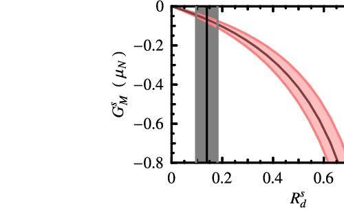
(Right) The pink band is the constraint for the proton strangeness magnetic moment from our data and the grey band indicates the given from Ref Leinweber et al. 2005.
Similarly, with the help of charge symmetry, one can estimate the of the proton via the root-mean-square radius from the up quark connected diagram Leinweber et al. 2006:
| (21) |
The left-hand side of Figure 10 shows the at each pion mass and their chiral extrapolation according to Ref. Dunne et al. 2002. Note that this is the result from analyzing the number of configuration listed in Table 2 only. Taking from chiral perturbation estimatesLeinweber et al. 2006, we find , which is consistent with experimental values, as shown on the right of Figure 10. The statistics will be further improved with the latest LHPC calculation.
 |
 |
III.3 Hyperon Axial Coupling Constants
The axial coupling constants, and , have important applications such as in hyperon scattering and non-leptonic decays. Previously, there only existed predictions from chiral perturbation theorySavage and Walden 1997 and large- calculations:
| (22) | |||
| (23) |
Figure 11 shows our lattice data and chiral extrapolation. Here we take a naive linear extrapolation against . We find numbers consistent with the models, and , but with much smaller errors.


IV Conclusion and Outlook
In summary, we report the latest nucleon calculations using RBC/UKQCD 2+1-flavor 3 fm DWF ensembles with pion masses as light as 310 MeV. Our calculations show good consistency with experimental values. Even those quantities, such as the first moments of the unpolarized quark distribution and helicity distribution, are chirally extrapolated to the physical pion mass in consistency with experimental values. We predict the zeroth moment of transversity, and we find the twist-3 matrix element to be consistent with zero.
In analyzing hyperon form factors, we use an indirect approach to get the strangeness of the proton magnetic moment, using mixed action. We find our dynamical result to be consistent with Adelaide-JLab Collaboration’s quenched result (which used a chiral correction for sea quark effects) and current experiments. The axial charge coupling of and baryons are also predicted with significantly smaller errorbars than estimated in the past. We will continue to increase statistics, especially in the light pion mass region to get even more accurate results in the future.
Acknowledgements
HWL thanks Riken-BNL center for their hospitality during work on the nucleon structure function and their support to make this trip; thanks also to collaborators Tom Blum, Shigemi Ohta, Kostas Orginos, Shoichi Sasaki and Takeshi Yamazaki for useful discussions; to Ross Young for discussion of strangeness physics and Anthony Thomas for helpful comments and discussions. The nucleon-structure calculations were done using the CPS on QCDOC with the resources of RBC collaboration, and the hyperon form factor calculations were performed using the Chroma software suiteEdwards and Joo 2005 on clusters at Jefferson Laboratory using time awarded under the SciDAC Initiative. Authored by Jefferson Science Associates, LLC under U.S. DOE Contract No. DE-AC05-06OR23177. The U.S. Government retains a non-exclusive, paid-up, irrevocable, world-wide license to publish or reproduce this manuscript for U.S. Government purposes.
References
- Kaplan (1992) D. B. Kaplan, Phys. Lett. B288, 342 (1992), eprint hep-lat/9206013.
- Kaplan (1993) D. B. Kaplan, Nucl. Phys. Proc. Suppl. 30, 597 (1993).
- Shamir (1993) Y. Shamir, Nucl. Phys. B406, 90 (1993), eprint hep-lat/9303005.
- Furman and Shamir (1995) V. Furman and Y. Shamir, Nucl. Phys. B439, 54 (1995), eprint hep-lat/9405004.
- Kogut and Susskind (1975) J. Kogut and L. Susskind, Phys. Rev. D11, 395 (1975).
- Orginos and Toussaint (1999) K. Orginos and D. Toussaint (MILC), Phys. Rev. D59, 014501 (1999), eprint hep-lat/9805009.
- Orginos et al. (1999) K. Orginos, D. Toussaint, and R. L. Sugar (MILC), Phys. Rev. D60, 054503 (1999), eprint hep-lat/9903032.
- Creutz (2006) M. Creutz, PoS LAT2006, 208 (2006), eprint hep-lat/0608020.
- Sharpe (2006) S. R. Sharpe, PoS LAT2006, 022 (2006), eprint hep-lat/0610094.
- Allton et al. (2007) C. Allton et al. (RBC) (2007), eprint hep-lat/0701013.
- Lin et al. (2007) H.-W. Lin, T. Blum, S. Ohta, K. Orginos, S. Sasaki, and T. Yamazaki, in preparation (2007).
- Orginos et al. (2006) K. Orginos, T. Blum, and S. Ohta, Phys. Rev. D73, 094503 (2006), eprint hep-lat/0505024.
- Sasaki et al. (2003) S. Sasaki, K. Orginos, S. Ohta, and T. Blum (the RIKEN-BNL-Columbia-KEK), Phys. Rev. D68, 054509 (2003), eprint hep-lat/0306007.
- Mathur and Dong (2001) N. Mathur and S.-J. Dong (Kentucky Field Theory), Nucl. Phys. Proc. Suppl. 94, 311 (2001), eprint hep-lat/0011015.
- Dong et al. (1998) S. J. Dong, K. F. Liu, and A. G. Williams, Phys. Rev. D58, 074504 (1998), eprint hep-ph/9712483.
- Lewis et al. (2003) R. Lewis, W. Wilcox, and R. M. Woloshyn, Phys. Rev. D67, 013003 (2003), eprint hep-ph/0210064.
- Foley et al. (2005) J. Foley et al., Comput. Phys. Commun. 172, 145 (2005), eprint hep-lat/0505023.
- Martinelli et al. (1995) G. Martinelli, C. Pittori, C. T. Sachrajda, M. Testa, and A. Vladikas, Nucl. Phys. B445, 81 (1995), eprint hep-lat/9411010.
- Gimenez et al. (1998) V. Gimenez, L. Giusti, F. Rapuano, and M. Talevi, Nucl. Phys. B531, 429 (1998), eprint hep-lat/9806006.
- Hemmert et al. (1998) T. R. Hemmert, B. R. Holstein, and J. Kambor, J. Phys. G24, 1831 (1998), eprint hep-ph/9712496.
- Hemmert and Weise (2002) T. R. Hemmert and W. Weise, Eur. Phys. J. A15, 487 (2002), eprint hep-lat/0204005.
- Hemmert et al. (2003) T. R. Hemmert, M. Procura, and W. Weise, Phys. Rev. D68, 075009 (2003), eprint hep-lat/0303002.
- Edwards et al. (2006) R. G. Edwards et al. (2006), eprint hep-lat/0610007.
- Gockeler et al. (2006) M. Gockeler et al., PoS LAT2006, 120 (2006), eprint hep-lat/0610118.
- Khan et al. (2006) A. A. Khan et al., Phys. Rev. D74, 094508 (2006), eprint hep-lat/0603028.
- Khan et al. (2004) A. A. Khan et al. (2004), eprint hep-lat/0409161.
- Dolgov et al. (2002) D. Dolgov et al. (LHPC), Phys. Rev. D66, 034506 (2002), eprint [http://arXiv.org/abs]hep-lat/0201021.
- Detmold et al. (2001) W. Detmold, W. Melnitchouk, J. W. Negele, D. B. Renner, and A. W. Thomas, Phys. Rev. Lett. 87, 172001 (2001), eprint hep-lat/0103006.
- Arndt and Savage (2002) D. Arndt and M. J. Savage, Nucl. Phys. A697, 429 (2002), eprint nucl-th/0105045.
- Chen and Savage (2002) J.-W. Chen and M. J. Savage, Nucl. Phys. A707, 452 (2002), eprint nucl-th/0108042.
- Detmold et al. (2002) W. Detmold, W. Melnitchouk, and A. W. Thomas, Phys. Rev. D66, 054501 (2002), eprint hep-lat/0206001.
- Orginos (2006) K. Orginos, PoS LAT2006, 018 (2006).
- Gockeler et al. (2001) M. Gockeler et al., Phys. Rev. D63, 074506 (2001), eprint hep-lat/0011091.
- Wandzura and Wilczek (1977) S. Wandzura and F. Wilczek, Phys. Lett. B72, 195 (1977).
- Bernard et al. (2001) C. W. Bernard et al., Phys. Rev. D64, 054506 (2001), eprint hep-lat/0104002.
- Aniol et al. (2006a) K. A. Aniol et al. (HAPPEX), Phys. Rev. Lett. 96, 022003 (2006a), eprint nucl-ex/0506010.
- Aniol et al. (2006b) K. A. Aniol et al. (HAPPEX), Phys. Lett. B635, 275 (2006b), eprint nucl-ex/0506011.
- Armstrong et al. (2005) D. S. Armstrong et al. (G0), Phys. Rev. Lett. 95, 092001 (2005), eprint nucl-ex/0506021.
- Spayde et al. (2004) D. T. Spayde et al. (SAMPLE), Phys. Lett. B583, 79 (2004), eprint nucl-ex/0312016.
- Maas et al. (2004) F. E. Maas et al. (A4), Phys. Rev. Lett. 93, 022002 (2004), eprint nucl-ex/0401019.
- Maas et al. (2005) F. E. Maas et al., Phys. Rev. Lett. 94, 152001 (2005), eprint nucl-ex/0412030.
- Leinweber (1996) D. B. Leinweber, Phys. Rev. D53, 5115 (1996), eprint hep-ph/9512319.
- Leinweber et al. (2005) D. B. Leinweber et al., Phys. Rev. Lett. 94, 212001 (2005), eprint hep-lat/0406002.
- Leinweber and Thomas (2000) D. B. Leinweber and A. W. Thomas, Phys. Rev. D62, 074505 (2000), eprint hep-lat/9912052.
- Yao et al. (2006) W. M. Yao et al. (Particle Data Group), J. Phys. G33, 1 (2006).
- Leinweber et al. (2006) D. B. Leinweber et al., Phys. Rev. Lett. 97, 022001 (2006), eprint hep-lat/0601025.
- Dunne et al. (2002) G. V. Dunne, A. W. Thomas, and S. V. Wright, Phys. Lett. B531, 77 (2002), eprint hep-th/0110155.
- Young (0900) R. D. Young (0900), eprint nucl-th/0609014.
- Savage and Walden (1997) M. J. Savage and J. Walden, Phys. Rev. D55, 5376 (1997), eprint hep-ph/9611210.
- Edwards and Joo (2005) R. G. Edwards and B. Joo (SciDAC), Nucl. Phys. Proc. Suppl. 140, 832 (2005), eprint hep-lat/0409003.