Poynting’s theorem for planes waves at an interface: a scattering matrix approach
Abstract
We apply the Poynting theorem to the scattering of monochromatic electromagnetic planes waves with normal incidence to the interface of two different media. We write this energy conservation theorem to introduce a natural definition of the scattering matrix . For the dielectric-dielectric interface the balance equation lead us to the energy flux conservation which express one of the properties of : it is a unitary matrix. For the dielectric-conductor interface the scattering matrix, that we denote by , is no longer unitary due to the presence of losses at the conductor. However, the dissipative term appearing in the Poynting theorem can be interpreted as a single absorbing mode at the conductor such that a whole , satisfying flux conservation and containing and this absorbing mode, can be defined. This is a simplest version of a model introduced in the current literature to describe losses in more complex systems.
pacs
41.20.Jb, 42.25.Bs, 42.25.Fx, 42.25.GyI Introduction
The scattering matrix is a useful tool to describe the multiple scattering that occur when planes waves enter to a system which in general is of complex nature, like atomic nucleus, chaotic and/or disordered systems, etc. Newton; Mello Although it is well known for particle waves in quantum mechanics Newton; Mello; Merzbacher; Cohen it can also be applied to any kind of plane waves. In the electromagnetic context the transfer matrix Jackson; Reitz is known instead of transfer1 but they are equivalent and related. Mello By definition, relates the outgoing plane waves amplitudes to the incoming ones to the system, from which the reflection and transmission coefficients are obtained; they are called reflectance and transmitance in electromagnetism. Reitz In the absence of dissipation, as happens in quantum electronic and some electromagnetic systems, becomes a unitary matrix, in particular . However, if the system contains a dissipative medium, is no longer unitary, in fact it is a sub-unitary matrix and , where the lack of unity is called absorbance in the electromagentic subject. Reitz
We are concerned with the electromagnetic case. There, a natural definition of through one of its properties arises from the Poynting theorem. This theorem is a energy balance equation which in the simplest form, i. e. for linear and non dispersive media, is given by Jackson
| (1) |
where
| (2) |
is the Poynting vector which gives the energy flux per unit area per unit time, and is the electromagnetic energy density
| (3) |
Here, we have assumed that the electric , electric displacement , magnetic induction , and magnetic fields, as well as the current density , are complex vectors whose real part only has physical meaning. We have also written explicitely the dependence on the position and time . The term in the right hand side of Eq. (1) is the negative of the work done by the fields per unit volume and represents the conversion of electromagnetic energy to thermal (or mechanical) energy. The version of Poynting’s theorem for dispersive media will not be touched here.
Our purpose in this paper is to apply the Poynting theorem to the simplest scattering system, an interface between two different media, to illustrate the relation of Poynting’s theorem and one property of . First, we will consider the absence of dissipation for the dielectric-dielectric interface for which the defined matrix is unitary. Second, the dissipative case is considered in the dielectric-conductor interface for which the scattering matrix, called , is sub-unitary. The last system is the simplest example to explain quantitatively a model, that we call the “parasitic channels” model, introduced in contemporary physics Lewenkopf1992; Brouwer1997 to describe complex systems with losses. Fyodorov2005 Also, could represents the scattering of an “absorbing patch” used to describe surface absorption. MM-M
The paper is organized as follows. In the next section we write the time averaged Poynting’s theorem and calculate the corresponding Poynting’s vector for planes waves and its flux through an open surface in a dielectric medium, as to be used in the sections that follow Sect. II. The dielectric-dielectric interface is considered in Sect. III while Sect. IV is devoted to the dielectric-conductor interface. Finally, we conclude in Sect. V
II Poynting’s theorem for linear and non-dispersive media
In what follows we will consider monocromatic high frequency oscillating fields such that
| (4) | |||||
| (5) | |||||
| (6) |
where have written the precise dependence on the spatial and temporal variables to avoid confusion due to the abuse of the notation. Here, the temporal average is of importance. Using the definition
| (7) |
for the average of a time dependent function over a period , the average of Eq. (1) can be written as
| (8) |
where we have used that, with help of Eqs. (4) and (5),
| (9) |
Also, by substitution of Eqs. (4) and (5) into Eq. (2), it is easy to see that
| (10) |
with (we write again the precise dependence)
| (11) |
being the time averaged Poynting’s vector. In equivalent way, using Eqs. (4) and (6), we get
| (12) |
Finally, the time averaged energy flux conservation law is given by
| (13) |
where only the real part has physical meaning.
If we integrate over a volume enclosed by a close surface , it says that the net flux of through is the negative of the work done by the fields if there are dissipative components in . I. e.,
| (14) |
where, from one side,
| (15) |
and, for the other side, using the divergence theorem can be written as a surface integral over as
| (16) |
II.1 Flux of Poynting’s vector for plane waves through an open surface of area
For a monocromatic plane wave with linear polarization in the axis, propagating along the positive -direction, the spatial component is
| (17) |
being the wave number, the index of refraction of the medium and the speed of light in vacuum; is a unit vector pointing in the positive -axis, and the complex number is the amplitude of . The magnetic field , calculated from using one of the Maxwell equations (Faraday’s law of induction), is
| (18) |
where is a unit vector pointing in the positive -direction and is the permeability of the free space (we have assumed a non-magnetic medium).

Sustituting Eqs. (17) and (18) into Eq. (11) we get
| (19) |
where is a unit vector pointing in the positive -axis. This equation means that the time averaged energy flux is constant along the propagation. If we consider an open surface of area as in Fig. 1, the flux of through it is (see Eq. (16))
| (20) |
where we have taken the normal unit vector of as .
III Poynting’s theorem at a dielectric-dielectric interface
Let us consider an interface between two dielectrics, with refractive indices and , in the plane as shown in Fig. 2. For the shake of simplicity, we consider plane waves with linear polarization in the axis with normal incidence on both sides of the interface. Therefore, the spatial part of the electric fields, on the left and on the right, are of the form
| (21) | |||||
| (22) |
where and ( and ) are the complex amplitudes of the incoming (outgoing) planes waves.
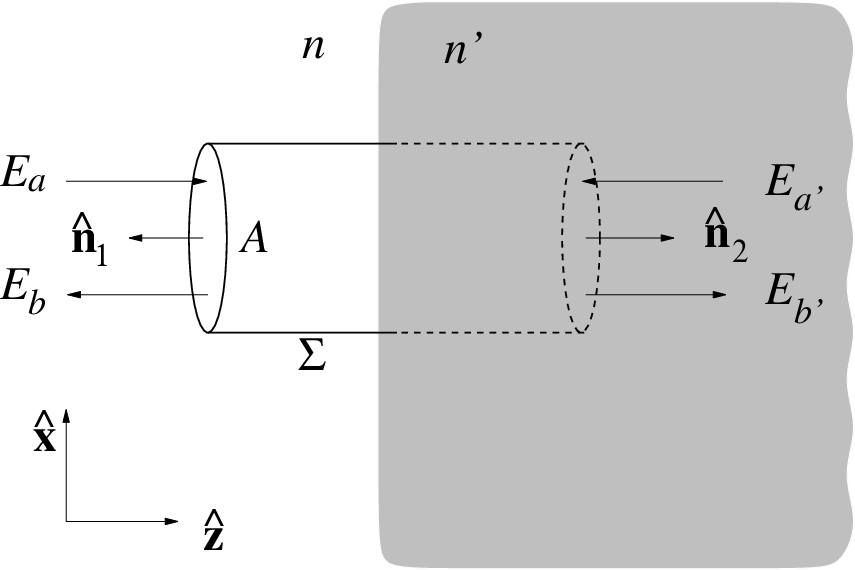
For this case, the right hand side of Eqs. (13) and (14) is zero () because there is not dissipation. Hence, . For convenience, we take a cylinder of cross section , including the covers, to be the closed surface (see Fig. 2). Due to normal incidence only the flux through the covers of section contribute to . Then, Eq. (14) gives
| (23) |
where () is the flux through one of the covers with normal unit vector (, 2) due to the -th plane wave; it is given by
| (24) |
With the convention that points outwards of , and are positive quantities while and are implicitely negative. Using the result of Eq. (20) for a plane wave, Eq. (23) can be written as
| (25) |
which can be arranged in a matricial form that we will use later, namely
III.1 The scattering matrix for the interface
By definition the Fresnel coefficients relate the outgoing to the incoming plane waves amplitudes as Jackson; Reitz; Marion
| (38) |
where is the matrix
| (39) |
The Fresnel coefficients of reflection , and transmission , are Jackson
| (40) | |||||
| (41) |
Although for this particular case they are real numbers, in general they are complex, in which case is a complex matrix. In order to be more general, in what follows we will assume that is complex.
By substitution of Eq. (38), Eq. (III) can be written as
from which we see that
| (54) |
or, equivalently,
| (55) |
where is the identity matrix and
| (56) |
is known in the literature as the scattering matrix which has the following general structure Mello
| (57) |
Here, and ( and ) are the reflection and transmission amplitudes for incidence on the left (right). From Eqs. (39), (40), (41) and (56) it is easy to see that
| (58) | |||||
| (59) |
Two remarks are worthy of mention. Mello The first one is that because the system described by is invariant under inversion of time, but in a more general context that is not necessary the case. Dyson The second is that because the optical path is not the same for the reflected trajectory when incidence is from right or left. Of course, Eq. (55) is satisfied in the case we are considering as can be easily checked using Eqs. (58) and (59). In particular,
| (60) |
where and are the reflection and transmission coefficients.
IV The dielectric-conductor interface
When one of the two media is a conductor with electric conductivity , the one on the right in Fig. 3 let say, the treatment is equivalent as in Sect. III but with a complex index of refraction: , where and are the optical constants. Reitz Also, the corresponding wave number becomes complex: we replace with
| (64) |
Then, on the conductor side the electric field is an evanescent wave while on the dielectric side we have incoming and outgoing plane waves. They are
| (65) | |||||
| (66) |
From Eq. (38), or Eq. (61), with we see that
| (67) | |||||
| (68) |
where and are obtained from Eqs. (58) and (59) but replacing by , namely
| (69) | |||||
| (70) |
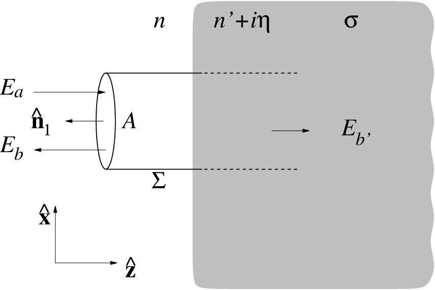
In this case, the scattering matrix of the system is and we denote it by . By definition (it is not necessary to normalize with respect to the index )
| (71) |
Comparing with Eq. (67) we see that
| (72) |
where, from Eqs. (69),
| (73) |
As for , the Poynting theorem impose a restriction to . To apply Eq. (14) we consider that the closed surface in Fig. 3 extends to infinity on the right of the interface, such that Eq. (15) gives
| (74) |
where we used that . Then, Eq. (14) can be written as
| (75) |
where the area has been cancelled. Using Eqs. (68) and (71), after an arrangement, Eq. (75) gives
| (76) |
meaning that is a subunitary matrix with the lack of unitarity (strength of absorption or absorbance),
| (77) |
The last equality is valid for metals in the upper infrared part of the spectrum and for metals at microwave and lower frequencies. Reitz-2 Of course as can be easily verified using Eqs. (73).
Eq. (76) can be seen as resulting of the unitarity condition for an -matrix that satisfy flux conservation (compare with Eq. (60)). This -matrix should has the structure (see Eq. (57))
| (78) |
where the phase can be taken as the phase of (see Eqs. (68) and (77)); using Eq. (70)
| (79) |
This form of says that the losses because of the conductor can be interpreted as due to a single mode of absorption whose “coupling” to the interface is . This is the simplest version of what we call the “parasitic channels” model Lewenkopf1992; Brouwer1997 appeared in the literature of contemporary physics in recent years to describe power losses in more complex systems (see Ref. Fyodorov2005 and references there in). That model consists in simulate losses with equivalent absorbing modes, each one having an imperfect coupling to the system. The total absorption is quantified by but and can not be determined separately. Our result not only explain this abstract model but quantify in an exact way the coupling of each absorbing mode as well the scattering matrix of a single absorbing patch in the surface absoprtion model. MM-M Our treatment presented here can also be used to construct artificially a system with multiple absorbing modes. drmmc
V Conclusiones
We reduced the time averaged Poynting theorem to a property of the scattering matrix. For that we applied this balance equation to a simplest scattering system, consisting of normally incident planes waves at an interface between two media. The simplest version of this theorem was used such that dispersive media and the corresponding dissipation were ignored. Two kind of interfaces were considered. In the first one, a dielectric-dielectric interface, the energy flux conservation leads to a natural definition of the scattering matrix which is restricted to be a unitary matrix. We recalled that the structure of reflects the symmetries present on the problem in other contexts. In the second one, the dielectric-conductor interface, the definiton of -matrix was used to describe the scattering taking into account the losses on the conductor side via the Poynting’s theorem. This allowed us introduce the parasitic channels model used in contemporary physics to describe the scattering with losses in more complex systems. We should were able to quantify the coupling of the single parasitic mode of absorption in our simple system. A system with multiple absorbing modes can be constructed and the results will be published elsewhere. Finally, the same treatement can be generalized for oblique incidence.
References
- (1) R. G. Newton, Scattering Theory of Waves and Particles (Springer, New York, 1982).
- (2) P. A. Mello and N. Kumar, Quantum Transport in Mesoscopic Systems (Oxford University Press, 2005).
- (3) E. Merzbacher, Quantum Mechanics (John Wiley & Sons, Inc., 1998), Third Edition.
- (4) C. Cohen-Tannoudji, B. Diu, and F. Laloë, Quantum Mechanics (John Wiley & Sons, 1997) Vol. 1.
- (5) J. D. Jackson, Classical Electrodynamics (John Wiley & Sons, Inc., 1999), Third Edition.
- (6) J. R. Reitz, F. J. Milford, and R. W. Christy, Foundations of Electromagnetic Theory (Addison-Wesley Company, Inc. 1993), Fourth Edition.
- (7) See for instance, problems 7.8 and 7.9 of Ref. Jackson, and 18.12 of Ref. Reitz.
- (8) C. H. Lewenkopf, A. Müller, and E. Doron, “Microwave scattering in an irregularly shaped cavity: Random-matrix analysis,” Phys. Rev. A 45, 2635-2636 (1992).
- (9) P. W. Brouwer and C. W. J. Beenakker, “Voltage-probe and imaginary-potential models for dephasing in a chaotic quantum dot,” Phys. Rev. B 55, 4695-4702 (1997).
- (10) Y. V. Fyodorov, D. V. Savin, and H.-J. Sommers, “Scattering, reflection and impedance of waves in chaotic and disordered systems with absorption,” J. Phys. A: Math. Gen. 38, 10731-10760 (2005).
- (11) M. Martínez-Mares and P. A. Mello, “Statistical wave scattering through classically chaotic cavities in the presence of surface absorption”, Phys. Rev. E 72, 026224 (2005).
- (12) J. B. Marion and M. A. Heald, Classical Electromagnetic Radiation (HBJ Publishers, 1980), Second Edition.
- (13) F. J. Dyson, “Statistical Theory of the Energy Levels of Complex Systems. I,” J. Math. Phys. 3, 140-156 (1962).
- (14) See equations 17-51, 17-63, and 17-64 of Ref. Reitz with the corresponding change of notation.
- (15) V. Domínguez-Rocha, M. Martínez-Mares, and E. Castaño, in preparation.