More hilltop inflation models
Abstract
Using analytic expressions, we explore the parameter space for hilltop inflation models with a potential of the form . With the positive sign and this converts the original hybrid inflation model into a hilltop model, allowing the spectral index to agree with the observed value . In some cases the observed value is theoretically favored, while in others there is only the generic prediction .
I Introduction
The general idea of what has been called bl hilltop inflation is that cosmological scales leave the horizon while the inflaton is near the top of a hill, with its potential still concave-downward. This allows the initial condition to be set by an era of eternal inflation, whose indefinite duration may remove any concern about the probability of arriving at the hilltop in the first place. Hilltop inflation also ensures that the spectral tilt is negative, though it may not be guaranteed that the amount of tilt is small as is required by observation.
It was noticed earlier bl that hilltop inflation is more natural than one might think. Starting with any rather flat potential, it is easy to generate a maximum with a reasonable-looking additional term. In this paper we pursue that line of thinking, by considering a potential which covers a range of possibilities, and is yet simple enough to yield analytic formulas for the predictions.
We shall take for granted the basic ideas of slow-roll inflation model-building, as explained for instance in treview; book; al; paris. Cosmological scales leave the horizon during about ten -folds of inflation. The value of the inflaton field when -folds of inflation remain is
| (1) |
where . Cosmological scales leave the horizon during about ten -folds of inflation, starting with the largest scale . (Here is the present value of the comoving wavenumber and the present Hubble parameter). For a standard cosmology after inflation, the value of when the latter scale leaves the horizon is typically in the range to . In following we give the predictions for .
We assume that the primordial curvature perturbation is generated from the vacuum fluctuation of the inflaton, instead of later by some curvaton-type mechanism. The spectrum of the tensor perturbation, as a fraction of the observed spectrum of the curvature perturbation, is , where . (Here and in the following all functions of are to be evaluated when the relevant scale leaves the horizon.) If the potential remains concave-downward for the rest of inflation, this implies bl
| (2) |
where is the variation of the inflaton field We will here demand only that the shape of the potential is such as to give . This is consistent with present observation.
The cmb anisotropy determines the magnitude of the spectrum of the curvature perturbation wmap3 as , with an uncertainty which is negligible in the present context. Invoking the slow-roll prediction for one finds
| (3) |
We call the second equality the cmb normalization. Our requirement corresponds to
| (4) |
The spectral index of the curvature perturbation is defined by
| (5) |
where is the number of -folds remaining after the scale leaves the horizon and the final equality assumes slow roll. The slow-roll prediction is
| (6) |
where . Assuming , the cmb anisotropy requires wmap3
| (7) |
An analysis including other types of observation combined finds instead . When we invoke the observational value we take the central value of the cmb result.
Now comes an important point. Since we are assuming , the observed value of means that we can take the prediction to be simply if it is to fit observation. We conclude that if a slow-roll model of inflation is to generate the observed curvature perturbation with , its potential must be concave-downward while cosmological scales leave the horizon, with .
We should also consider the running . The models we consider here give and this condition should be imposed as a prior when determining the upper bound on allowed by observation. As will be shown elsewhere klm, current observations require in that case something like . We impose this constraint where relevant.
II The potential
We consider a potential of the following form, with positive.
| (8) | |||||
| (9) |
with
| (10) |
The additional terms are presumed negligible during inflation and we require that rolls towards the origin. There is no need to assume that is integral if this is just regarded as a parameterisation of the potential.
To justify keeping just two terms, especially if is an integer, we would like after the largest cosmological scale leaves the horizon (which we are taking to correspond to ). We will just require that the maximum of and is .
We consider three different regimes of and .
- 1.
Two-term approximation about the hilltop. The choice and sets at the hilltop, and adds a higher power to the quadratic term. This is sketched in Figure 1.
- 2.
Hilltop mutated/brane hybrid inflation. The choice and converts these models to hilltop models, as sketched in Figure 2.
- 3.
Hilltop tree-level hybrid inflation. The choice and converts the original hybrid inflation model to a hilltop model, as illustrated in Figure 3.
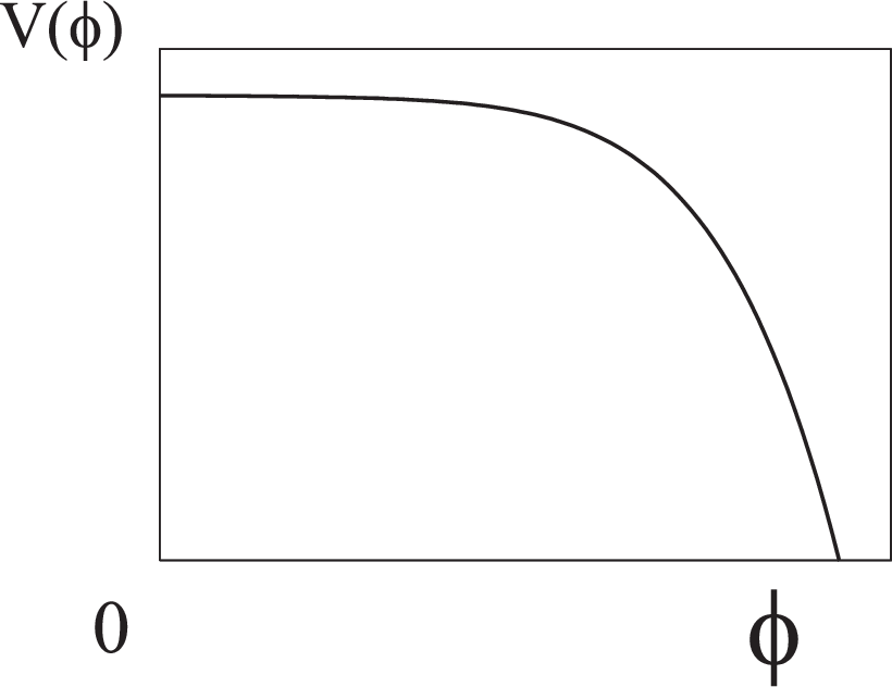


To achieve slow-roll with the potential (9), we need giving
| (11) | |||||
| (12) |
Then Eq. (1) has the analytic solution grs
| (13) | |||||
| (14) |
leading to the predictions
| (15) | |||||
| (16) | |||||
| (17) | |||||
In a supergravity theory where vanishes in the global supersymmetric limit, the generic expectation is . For slow-roll inflation per se, all we need is which does not necessarily imply significant fine-tuning. The problem (usually called the problem) comes though when one tries to understand why the spectral index given by Eq. (6) is so close to 1. We will keep this issue in mind, and review the final situation in the Conclusion after considering in turn each of the three cases.
III Two-term approximation
The two-term approximation may apply in a wide variety of cases, and has a long history. In using our parameterisation we choose the origin to be a maximum of (at least in the regime . The necessary condition might be ensured by a symmetry (with the origin the fixed point of the transformation) but that is not essential. The maximum of the potential might be occur because the potential is periodic (corresponding to being a pseudo Nambu-Goldstone boson (PNGB)) or else through the interplay of two terms as in our cases 2 and 3.
We will focus on the non-hybrid case, where descends smoothly to a minimum with . Then we might be dealing with modular inflation corresponding to . (‘Moduli’ allowing this kind of inflation may be expected in string theory as discussed for instance in racetrack.) Alternatively we might be dealing with a small-field model, corresponding to some orders of magnitude below . If the origin is a fixed point of symmetries involving we deal with what one might call new inflation. (The original new inflation model new (see also hm) corresponds more or less to and which we consider below.)
This case has been investigated in grs; grslett, where the formulas Eqs. (13)–(16) were first given.11 1 These authors had in mind the case of new inflation. Less complete investigations were made earlier, keeping just the term treview; al; paris, both terms with dineriotto; treview; pseudonatural, and both terms with generic supernew.) In the following we present a further investigation of this interesting case.
III.1 Spectral index
The potential is concave-downward throughout inflation. As a parameterization over a limited range it makes sense to allow to be non-integral, with .
Since is increasing during inflation, one expects the value of given by Eq. (1) to be insensitive to , at least some part of the parameter space. That would correspond to being a good approximation. We will not make that approximation, but instead take (the point at which slow-roll fails) to be the point where which corresponds to or
| (18) |
Since slow-roll requires , our requirement becomes
| (19) |
Using Eq. (18) we find that the spectral index depends only on and . For we recover the known result treview
| (20) |
This is automatically within the observed range.
For we recover the known result
| (21) |
In that case, the requirement requires corresponding to . The value of is in mild conflict with the slow-roll requirement, and of course the value of is far below the observed one.
In Figure 4 we plot contours of constant in the - plane. The nearly horizontal lines correspond to the limit (20). The nearly vertical lines correspond to the limit (21) being practically attained at , the term of V proportional to ensuring that slow-roll ends at .


III.2 Modular inflation
We now look at the cmb normalization, beginning with modular inflation. Here the minimum of is expected to be of order , corresponding roughly to . We will impose that equality, leaving only the parameters and .
As is not far below we should view Eq. (9) just as an approximation, valid hopefully for some . In Figure 6 we plot the cmb-normalized against , for a few values of and the range . This plot shows if we demand a high inflation scale in a modular inflation, then in a modular inflation model cannot be far below .

III.3 New inflation
For new inflation corresponding to , it is reasonable to suppose that the term is the leading next term in a power-series expansion, further terms being suppressed by the small value of . Then will be an integer bigger than 2. The integer can be bigger than 3 because in new inflation the origin is supposed to be a fixed point of symmetries.
III.3.1 Case
Let us suppose that odd are forbidden by a symmetry , making the leading term . This gives the original new inflation model new, except that the slight running of with invoked there is absent. A famously small value of is required. The original version of the model, where is a gauge coupling, was therefore rejected but it was soon pointed out sv that could instead be a Yukawa coupling making the small value perhaps acceptable. More recently it has been noticed ss that the predicted spectral index is compatible with observation.
In the version of the last paragraph this model is not supersymmetric so that there is no natural expectation that will be significant, but still we are free to consider that case. Moreover, this potential with significant has been motivated in other ways, both non-supersymmetric pseudonatural and supersymmetric dineriotto. The second case however very fine-tuned treview. It therefore appears that the case is best realised without supersymmetry, especially if is included.
After imposing the cmb normalization there is one parameter which we take to be . In Figure 7 we show and as functions of . We see in Figure 7 that increasing decreases both and , allowing the latter to be well below the observed value.

III.3.2 Case
The need for the quartic term to be very suppressed is a generic feature of inflation models after the cmb normalization is imposed treview. Supposing it to be negligible and still taking to be even, we expect the leading term to be .
In Figure 8, we show contours of in the - plane, assuming that is given by Eq. (18). We also show the lines and . In Figures 9 and 10 we show against . From Figure 10 , we can see the spectral index can be far below the observed value.
To suppress the quartic term we would like to impose supersymmetry. With a minimal Kahler potential we arrive at the case with a superpotential of the form supernew
| (22) |
where the extra terms ensure without affecting the potential in the direction of the inflaton .


IV Hilltop mutated hybrid inflation
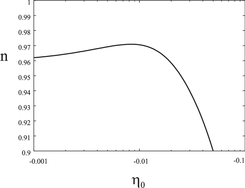
Now we come to the second case, characterized by and . The prediction for is given in Figure 5. Regarding the limit of large and small , the remarks made for the previous case apply.
This case corresponds to what is called mutated hybrid inflation mut; smooth; ourmut. It differs from ordinary hybrid inflation in the following respect. Ordinary hybrid inflation assumes a coupling between the inflaton field and the waterfall field which is some function of times . This fixed at the origin during slow-roll inflation, which ends when passes through some critical value which destabilizes . In mutated hybrid inflation, the coupling involves a higher power than . As a result, the waterfall field is not fixed, but instead adjusts to minimize the potential as the inflaton field slowly rolls. The inflationary potential is and inflation ends when slow-roll fails.
Until now, it has usually been assumed that with is absolutely flat. The most general potential that has been considered ourmut is then
| (23) |
When the potential is minimized by at fixed , the potential becomes
| (24) |
This is of the form Eq. (9) with and . If is a fixed point of the symmetries, it is quite reasonable to add a term to the above potential, to arrive at Eq. (9). More generally though, a linear term would be allowed in the potential and so it would be more reasonable to add a term with a parameter.
The latter is the case for the original mutated hybrid inflation model mut. It is not covered by our parameterisation, and we focus instead on what was called smooth hybrid inflation smooth. There the origin is a fixed point, with
| (25) |
During inflation we can drop the term, to get Eq. (23) with , and . This leads Eq. (9) with and
| (26) |
and of course . We can easily compare this with smooth. First, we use equation (11), and take the limit for . We obtain , this is exactly the same as smooth. Second, we can see from (10) and use the relation , we obtain . Use the above relation we can solve for .
The inclusion of a no-zero for smooth hybrid inflation has been considered in rss and we further investigate it now. In Figure 12 we see that cannot be very big. From Figures 11 and 14 we see that this requires a high inflation scale, and a spectral index around the observed value.

The case has also been derived in a colliding brane scenario collbrane. Our potential does not apply in that case, because the origin will not be a fixed point of symmetries so that a linear term in is allowed which would go beyond our parameterisation. (Also, non-canonical normalization is allowed in this case, though there is a significant regime of parameter space where the normalization is canonical.)


We also considered mutated hybrid inflation with , assuming that the origin is a fixed point of the symmetries. We plot the spectral index against in Figs 15 and 16 for . These plots show that basically we can have a big range of spectral index by introducing nonzero in our models.


V - and -term inflation
Now we consider the standard - and -term inflation models fterm; dterm. Here, sticking to the simplest versions of those models, is replaced by with a constant of order . Since we are assuming , other, this is equivalent to take the limit with fixed at the value
| (27) |
This case has been analyzed for both positive panag; mydterm; km and bl; john negative , but the latter choice leading to hilltop inflation is more interesting and makes it easier for the models to agree with observation and we analyze it further now.
We find
| (28) |
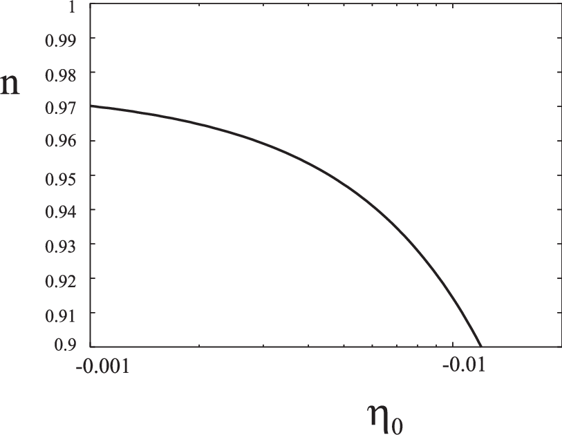
which is independent of . This is shown in Figure 18. We see that the requirement requires .
The cmb normalization is
| (30) |
This is plotted in Figure 20. In both the - and -term models, is the vev of the waterfall field. In the -term case one supposes that the waterfall field is a GUT Higgs field making its vev of order the GUT scale , and a similar value is expected in the -term case with a high string scale. Imposing that restriction, we see from Figure 19 that cannot be far below the observed value.


VI Hilltop tree-level hybrid inflation
VI.1 Generic case
The third case has never been considered before. Here we are seeing whether the original hybrid inflation model andreihybrid, which gives in contradiction with observations, can be saved by the addition of the term, as in in Figure 3.
In this case we keep as a parameter of the model. The value of depends on . If the coupling of the inflaton to the waterfall field is , then (where is the tachyonic mass of the waterfall field. This gives
| (31) |
The plausible range of is clearly very large.
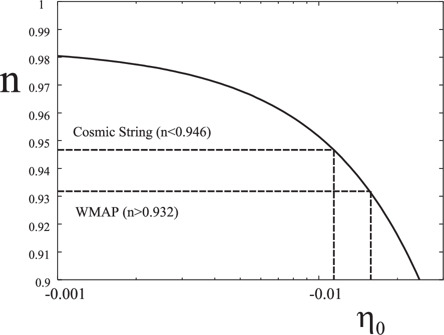
To obtain a general idea about the allowed parameter space, we shall fix (the central observed value). Consider first the case . In Figure 21 we show and as a function of . At , , which is also the line above which we have . The curve of against also represent the contour of in the - plane. We can generalize this for which we plot in Figure 22. In Figure 22, we also show the upper bound for , which is provided by .
Now consider . In Figure 23 we show in the - plane contours of and contours of . We also show the lines and . The trapezium-like area (on the r.h.s. of (which means ) and ) represents the allowed region for the inflation model. The upper horizontal line represents , underneath which is the requirement . The lower horizontal line is , above which is the requirement corresponding to motion towards . Using equation (10) and (11), we can see at , which makes therefore and for all finite . That is why the plot of and behaves odd there.


In Figure 21, we see that has to be very small, in accordance with the known generic result. On the assumption that it will actually be negligible after suppression by (say) a supersymmetry mechanism, we choose instead , to obtain the plot shown in Figure 23.
The term in the potential proportional to may be regarded as parameterizing physics beyond the ultra-violet cutoff. Taking the cutoff to be , one might generically expect in . With a lower cutoff one might expect in (equivalent to with the replacement .
Within the context of supersymmetry, a simple realization of hybrid inflation has been termed supernatural supernatural inflation. Here, the superpotential provides only the coupling between the waterfall field and the inflaton. All other terms in the potential, including come from soft supersymmetry breaking. As in the generic case, our addition of the term proportional to can rescue the model by allowing it to give a spectral index in agreement with observation.
VI.2 Black hole formation
As sketched in Figure 3, the potential starts out concave-downward as required by observation, but then turns up. As a result it can be much flatter at the end of inflation than when cosmological scales leave the horizon. This allows at the end of inflation to be much bigger than the observed value and the question arises whether it can be of order or so, leading to the production of black holes.
After fixing and apply the cmb normalization, for both the cases and , we can express and as a function of . We show the plots of versus for the case and in Figure 24 and 25. It is seen that black hole formation would require running , far in excess of what is allowed by observation.
It is clear that any potential allowing black hole formation will have a shape like the one in Figure 3. In a companion paper klm it is shown that suitable potentials definitely exist. A well-motivated example that seems viable at present is the running-mass model running. With the parameters used for Figure 2 of lgl, black hole formation is possible with . By altering the gauge group it should be possible to achieve black hole formation with a lower .


VII Conclusion
We have extended the investigation of bl, demonstrating that hilltop inflation is an absolutely generic possibility for both hybrid and non-hybrid inflation models. This is a welcome development, in that it allows a whole range of models to fit observation while being at the same time well-motivated from the particle physics viewpoint. The development is disturbing though, in that it muddies the clean classification of the models presented in for instance treview which could formerly be made on the basis of the sign and likely value of the spectral index. However, discrimination between the models will still be possible if the running can be measured with an accuracy (ie. an order of magnitude better than the bound klm provided by present data).
We have explored the parameter space of each model after imposing the cmb normalization on the spectrum. Regarding the spectral index, we have exhibited the effect of imposing the observed value , but we have also asked what range would have been allowed theoretically. The latter question is reasonable, because in contrast with the normalization of the spectrum there does not seem to be any anthropic constraint on the spectral index. Therefore, one would like a value in the right ball-park to be an automatic consequence of imposing the cmb normalization.
This desirable state of affairs seems to be achieved for the case of smooth hybrid inflation and -term inflation, when we require that these models be part of a GUT theory. It also seems to be the case for -term inflation and modular inflation, if we require a high inflation scale corresponding to a high string scale.
In other cases, including new inflation, the spectral index might have taken any value in the range demanded by slow-roll. Tree-level hybrid inflation even allows the whole range . It was pointed out some time ago bdl that the same is true for -term inflation aterm, where one deals with a potential that is well-approximated by
| (32) |
(The same kind of potential has been found recently recentmod in the context of colliding brane inflation.) With this potential, has a maximum in about half of the parameter space, giving a hilltop model. Therefore, if hilltop inflation is favored on the ground that eternal inflation can provide the initial condition these models automatically give but they do not automatically place close to 1.
There is a proposal racetrack even in these cases, for understanding why is so close to 1. This is to demand as much slow-roll inflation as possible, so that the inflated volume created by slow-roll is as large as possible. Indeed this demand will drive as close to 1 as is allowed by the parameter space. For new inflation and modular inflation we have argued that the demand will make of order a few divided by placing it in the right ball-park. For tree-level hybrid inflation and the potential (32) the demand will instead drive to be indistinguishable from 1. In any case, it is not clear to us why one should want to maximise the amount of slow-roll inflation, if there has already been a much larger amount of eternal inflation.
Acknowledgments. The research is supported by PPARC grants PPA/G/S/2003/00076 and PP/D000394/1 and by EU grants MRTN-CT-2004-503369 and MRTN-CT-2006-035863. DHL thanks Liam McAllister for valuable correspondence about colliding-brane inflation.
References
- (1) L. Boubekeur and D. H. Lyth, JCAP 0507, 010 (2005)
- (2) D. H. Lyth and A. Riotto, Phys. Rept. 314, 1 (1999)
- (3) A. R. Liddle and D. H. Lyth, Cosmological Inflation and Large Scale Structure, (CUP, Cambridge, 2000)
- (4) L. Alabidi and D. H. Lyth, JCAP 0605, 016 (2006).
- (5) D. H. Lyth, arXiv:hep-th/0702128.
- (6) D. N. Spergel et al., arXiv:astro-ph/0603449.
- (7) J. Lesgourgues, M. Viel, M. G. Haehnelt and R. Massey, arXiv:0705.0533 [astro-ph].
- (8) K. Kohri, D.H. Lyth and A. Melchiorri (2007) in preparation.
- (9) G. German, G. G. Ross and S. Sarkar, Nucl. Phys. B 608, 423 (2001) [arXiv:hep-ph/0103243].
- (10) G. German, G. G. Ross and S. Sarkar, Phys. Lett. B 469, 46 (1999)
- (11) J. J. Blanco-Pillado et al., JHEP 0609, 002 (2006) [arXiv:hep-th/0603129].
- (12) A. D. Linde, Phys. Lett. B 108, 389 (1982); A. Albrecht and P. J. Steinhardt, Phys. Rev. Lett. 48, 1220 (1982).
- (13) Q. Shafi and A. Vilenkin, Phys. Rev. Lett. 52 (1984) 691.
- (14) Q. Shafi and V. N. Senoguz, Phys. Rev. D 73 (2006) 127301 [arXiv:astro-ph/0603830].
- (15) Hawking, S. W., and Moss, I. G., 1982, Phys. Lett. B 110, 35.
- (16) c E. J. Copeland, A. R. Liddle, D. H. Lyth, E. D. Stewart and D. Wands, Phys. Rev. D 49 (1994) 6410; E. D. Stewart, Phys. Rev. D 51 (1995) 6847; G. R. Dvali, Q. Shafi and R. K. Schaefer, Phys. Rev. Lett. 73, 1886 (1994).
- (17) E. D. Stewart, Phys. Rev. D 51, 6847 (1995); P. Binetruy and G. R. Dvali, Phys. Lett. B 388 (1996) 241; E. Halyo, Phys. Lett. B 387 (1996) 43.
- (18) C. Panagiotakopoulos, Phys. Lett. B 402 (1997) 257; C. Panagiotakopoulos, Phys. Rev. D 55 (1997) 7335.
- (19) D. H. Lyth, Phys. Lett. B 419 (1998) 57.
- (20) C. F. Kolda and J. March-Russell, Phys. Rev. D 60 (1999) 023504.
- (21) C. M. Lin and J. McDonald, Phys. Rev. D 74, 063510 (2006).
- (22) E. D. Stewart, Phys. Lett. B 345, 414 (1995).
- (23) G. Lazarides and C. Panagiotakopoulos, Phys. Rev. D 52 (1995) 559.
- (24) D. H. Lyth and E. D. Stewart, Phys. Rev. D 54, 7186 (1996)
- (25) M. ur Rehman, V. N. Senoguz and Q. Shafi, Phys. Rev. D 75 (2007) 043522 [arXiv:hep-ph/0612023].
- (26) G. R. Dvali and S. H. H. Tye, Phys. Lett. B 450, 72 (1999).
- (27) A. D. Linde, Phys. Rev. D 49 (1994) 748.
- (28) S. H. Henry Tye, arXiv:hep-th/0610221.
- (29) N. Arkani-Hamed, H. C. Cheng, P. Creminelli and L. Randall, JCAP 0307, 003 (2003) [arXiv:hep-th/0302034].
- (30) M. Dine and A. Riotto, Phys. Rev. Lett. 79, 2632 (1997) [arXiv:hep-ph/9705386].
- (31) K. Kumekawa, T. Moroi and T. Yanagida, Prog. Theor. Phys. 92 (1994) 437 [arXiv:hep-ph/9405337]; K. I. Izawa and T. Yanagida, Phys. Lett. B 393 (1997) 331 [arXiv:hep-ph/9608359]; K. I. Izawa, M. Kawasaki and T. Yanagida, Phys. Lett. B 411 (1997) 249 [arXiv:hep-ph/9707201]; K. I. Izawa, Phys. Lett. B 576 (2003) 1 [arXiv:hep-ph/0305286]; M. Ibe, K. I. Izawa, Y. Shinbara and T. T. Yanagida, Phys. Lett. B 637 (2006) 21 [arXiv:hep-ph/0602192].
- (32) L. Randall, M. Soljacic and A. H. Guth, Nucl. Phys. B 472, 377 (1996) [arXiv:hep-ph/9512439].
- (33) E. D. Stewart, Phys. Lett. B 391, 34 (1997) [arXiv:hep-ph/9606241]; E. D. Stewart, Phys. Rev. D 56, 2019 (1997) [arXiv:hep-ph/9703232]; L. Covi and D. H. Lyth, Phys. Rev. D 59, 063515 (1999) [arXiv:hep-ph/9809562].
- (34) S. M. Leach, I. J. Grivell and A. R. Liddle, Phys. Rev. D 62, 043516 (2000) [arXiv:astro-ph/0004296].
- (35) R. Allahverdi, K. Enqvist, J. Garcia-Bellido and A. Mazumdar, Phys. Rev. Lett. 97, 191304 (2006) [arXiv:hep-ph/0605035]; R. Allahverdi, K. Enqvist, J. Garcia-Bellido, A. Jokinen and A. Mazumdar, JCAP 0706, 019 (2007) [arXiv:hep-ph/0610134].
- (36) J. C. Bueno Sanchez, K. Dimopoulos and D. H. Lyth, JCAP 0701, 015 (2007) [arXiv:hep-ph/0608299].
- (37) D. Baumann, A. Dymarsky, I. R. Klebanov, L. McAllister and P. J. Steinhardt, arXiv:0705.3837 [hep-th]; D. Baumann, A. Dymarsky, I. R. Klebanov and L. McAllister, arXiv:0706.0360 [hep-th]; A. Krause and E. Pajer, arXiv:0705.4682 [hep-th].