INSTITUT NATIONAL DE RECHERCHE EN INFORMATIQUE ET EN AUTOMATIQUE
Recent Advances in Solving the Protein Threading Problem
Rumen Andonov --- Guillaume Collet††footnotemark:
--- Jean-François Gibrat --- Antoine Marin††footnotemark:
— Vincent Poirriez — Nikola Yanev
N° 6253
July 2007
Recent Advances in Solving the Protein Threading Problem
Rumen Andonov, Guillaume Collet00footnotemark: 0 , Jean-François Gibrat, Antoine Marin00footnotemark: 0 , Vincent Poirriez, Nikola Yanev
Thème BIO — Systèmes biologiques
Projets Symbiose
Rapport de recherche n° 6253 — July 2007 — ?? pages
Abstract: The fold recognition methods are promissing tools for capturing the structure of a protein by its amino acid residues sequence but their use is still restricted by the needs of huge computational resources and suitable efficient algorithms as well. In the recent version of FROST (Fold Recognition Oriented Search Tool) package the most efficient algorithm for solving the Protein Threading Problem (PTP) is implemented due to the strong collaboration between the SYMBIOSE group in IRISA and MIG in Jouy-en-Josas. In this paper, we present the diverse components of FROST, emphasizing on the recent advances in formulating and solving new versions of the PTP and on the way of solving on a computer cluster a million of instances in a reasonable time.
Key-words: Protein Threading Problem, Protein Structure, Parallel Processing
Nouvelles avancées dans la reconnaissance de repliements
Résumé : Parmi les méthodes informatiques permettant de trouver la structure d’une protéine à partir de sa seule séquence, les méthodes par reconnaissance de repliements semblent prometteuses. Néanmoins, ces méthodes demandent une très grande quantité de ressources ainsi que des algorithmes performants. Le logiciel FROST (Fold Recognition Oriented Search Tool) implémente une méthode de reconnaissance de repliement qui est le fruit d’une étroite collaboration entre l’équipe Symbiose de l’IRISA et l’unité MIG de l’INRA de Jouy-en-Josas. Nous présentons ici les différentes composantes de FROST et les dernières avancées réalisées afin de résoudre efficacement le problème du Protein Threading. En particulier, nous présentons une version parallélisée de FROST permettant de résoudre un grand nombre d’instances en un temps raisonnable.
Mots-clés : Reconnaissance de repliement, structure des protéines, parallélisation
1 Introduction
Genome sequencing projects generate an exponentially increasing amount of raw genomic data. For a number of organisms whose genome is sequenced, very little is experimentally known, to the point that, for some of them, the first experimental evidence gathered is precisely their DNA sequence. In the absence, or extreme paucity, of experimental evidences, bioinformatic methods play a central role to exploit the raw data. The bioinformatic process that extracts biological knowledge from raw data is known as annotation.
Annotation is composed of two phases:
- 1.
a static phase whose purpose is to describe the basic “objects” that are found in the genome: the genes and their products the proteins.
- 2.
a dynamic phase that seeks to describe the processes, i.e., the complex ways genes and proteins interact to create functional networks that underly the biological properties of the organism.
The first phase is the cornerstone of the annotation process. The first step consists in finding the precise location of genes on the chromosome. Then, for those genes that encode proteins, the next step is to predict the associated molecular, cellular and phenotypic functions. This is often referred to as in silico functional annotation. Different methods exist for predicting protein functions, the most important of which are based on properties of homologous proteins.
Homology is a key concept in biology. It refers to the fact that two proteins are related by descent from a common ancestor. Homologous proteins have the following properties:
- •
they may have sequences that, despite the accumulated mutations, still resemble the ancestor sequence;
- •
their three-dimensional structures are similar to the structure of the ancestor;
- •
they may have conserved the ancestor function, or at least a related function.
Therefore the principle of in silico functional analysis, based on homology searches, is to infer a homology relationship between a protein whose function is known and the new protein under study then to transfer the function of the former to the latter.
The inference of the homology relationship is based on the previously listed properties of homologous proteins. The first methods developed used the first property, the conservation of the sequences, and were based on sequence comparisons using alignment tools such as PSI-BLAST [1].
These methods are still the workhorses of in silico functional annotation: they are fast and endowed with a very good statistical criterion allowing to judge when two proteins are homologous. Unfortunately they also have a drawback. They are very inefficient when the proteins under study happen to be remote homologs, i.e., when their common ancestor is very ancient. In such a case the sequences may have undergone many mutations and they are no longer sufficiently similar for the proteins to be recognized as homologous.
For instance, when analyzing prokaryote genomes, these techniques cannot provide any information about the function of a noticeable fraction of the genome proteins (between 25% and 50% according to the organism studied). Such proteins are known as “orphan” proteins. One also speaks of orphan families when several homologous proteins are found in newly sequenced genomes that cannot be linked to any protein with a known function.
To overcome this problem new methods have been developed that are based on the second property: the good conservation of the 3D structure of homologous proteins. These methods are known as threading methods, or more formally, as fold11 1 in this context fold refers to the protein 3D structure recognition methods.
The rational behind these methods is threefold:
- 1.
As mentioned above, 3D structures of homologous proteins are much better conserved than the corresponding amino acid sequences. Numerous cases of proteins with similar folds and the same function are known, though having less than 20% sequence identity [2].
- 2.
There is a limited, relatively small, number of protein structural families. Exact figures are still a matter of debate and vary from 1 000 [3] to at most a few thousands [4]. According to the statistics of the Protein Data Bank (PDB)22 2 http://www.rcsb.pdb/ there are about 700 (CATH definition [5]) or 1 000 (SCOP definition [6]) different 3D structure families that have been experimentally determined so far.
- 3.
Different types of amino acids have different preferences for occupying a particular structural environment (being in an -helix, in a -sheet, being buried or exposed). These preferences are the basis for the empirically calculated score functions that measure the fitness of a given alignment between a sequence and a 3D structure.
Based on these facts, threading methods consist in aligning a query protein sequence with a set of 3D protein structures to check whether the sequence might be compatible with one of the structures. These methods consist of the following components:
- •
a database of representative 3D structural templates;
- •
an objective function (score function) that measures the fitness of the sequence for the 3D structure;
- •
an algorithm for finding the optimal alignment of a sequence onto a structural template (with respect to the objective function);
- •
a statistical analysis of the raw scores allowing the detection of the significant sequence-structure alignments.
To develop an effective threading method all these components must be properly addressed. A description of the implementation of these different components in the FROST (Fold Recognition Oriented Search Tool) method [7] is detailed in the next section. Let us note that, from a computer scientist’s viewpoint, the third component above is the most challenging part of the treading method development. It has been shown that, in the most general case, when variable length alignment gaps are allowed and pairwise amino acid interactions are considered in the score function, the problem of aligning a sequence onto a 3D structure is NP-hard [8]. Until recently, it was the main obstacle to the development of efficient threading methods. During the last few years, much progress has been accomplished toward a solution of this problem for most real life instances [9, 10, 11, 12, 13, 14].
Despite these improvements, threading methods, like a number of other bioinformatic applications, have high computational requirements. For example, in order to analyze the orphan proteins that are found in prokaryote genomes, a back of the envelop computation shows that one needs to align 500 00033 3 This figure corresponds to the number of sequenced genomes (500) times the average number of proteins per genome (3 000) times the mean fraction of orphan proteins () protein sequences with at least 1 000 3D structures. This represents 500 millions alignments. Solving such quantity of alignments is, of course, not easily tractable on a single computer. Only a cluster of computers, or even a grid, can manage such amount of computations. Fortunately, as we will show hereafter, it is relatively straightforward to distribute these computations on a cluster of processors or over a grid of computers.
Grids are emerging as a powerful tool to improve bioinformatic applications effectiveness, particularly for protein threading. For example, the encyclopedia of life project [15] integrates 123D+ threading package in its distributed pipeline. All the pipeline processes, from DNA sequence to protein structure modeling, are parallelized by a grid application execution environment called APST (for Application-level scheduling Parameter Sweep Template). Another distributed pipeline for protein structure prediction is proposed by T. Steinke and al. [16]. Their pipeline consists in three steps : a pre-processing phase by sequence alignments, a protein threading phase and a final 3D refinement. Their threading algorithm solves the alignment problem by a parallel implementation of a Branch-&-Bound optimizer using the score function of Xu and al. [17]. With a cluster of 16 nodes, they divided by 2 the computation-time of aligning 572 sequences with about 37 500 structures from the PDB.
To maintain a structural annotation database up to date (project e-protein44 4 http://www.e-protein.org/), McGuffin and colleagues describe a fold recognition method distributed on a grid with the JYDE (Job Yield Distribution Environment) system which is a meta-scheduler for clusters of computers. To annotate the human genome, they use their mGen THREADER software integrated with JYDE on three different grid systems. On these three independent clusters of 148, 243 and 192 CPUs (515 CPUs), the human genome annotations can be updated in about 24 hours.
The rest of this chapter is organized as follows. In section 2 we present basic features of the FROST method. Section 3 further details the mathematical techniques used to tackle the difficult problem of aligning a sequence onto a 3D structure. Section 4 introduces the different operations required in FROST to make the entire procedure modular and describes how the modules can be distributed and executed in parallel on a cluster of computers. Computational benchmarks of the parallelized version of FROST are presented in section 5. In section 6 we discuss future research directions.
2 FROST: a fold recognition method
2.1 Definition of protein cores
Threading methods require a database of representative 3D structures. The Protein Data Bank (PDB) that gathers all publicly available 3D structures contains about 40 000 structures. However this database is extremely redundant. Analyses of the PDB show that it contains at most about 1 000 different folds [6]. In theory only these folds need to be taken into consideration. In practice, to obtain a denser coverage of the 3D structure space, the PDB proteins are clustered into groups having more than 30% sequence identity and the best specimen of each group (in terms of quality of the 3D structure : high resolution, small R-factor, no, or few, missing residues) is selected. The final database contains about 4 500 3D structures.
For the purpose of fold recognition, the whole 3D structure is not required, only those parts of the structure which are characteristic of the structural family need to be considered. This leads to the notion of structural family core. The core is defined as those parts that are conserved in all the 3D structures of the family and are thus distinctive of the corresponding fold.
There are two practical reasons for using cores:
- 1.
aligning a sequence onto portions of the 3D structure that are not conserved is likely to introduce a noise that would make the detection process more difficult;
- 2.
by definition, no insertion or deletion is permitted within core elements since, otherwise, they would not be conserved parts of the family structures.
In protein families often one observes that the conserved framework of the 3D structure consists of the periodic secondary structures, helices and strands, the loops at the surface of the protein are variables. Accordingly, in FROST the core of the protein structures is defined as consisting of the helices and strands.
Hereafter we will refer to cores instead of 3D structures or folds.
2.2 Score function
To evaluate the fitness of a sequence for a particular core we need an objective (or score) function. There are two categories of score functions: “local” and “non local”. The former ones are, in essence, similar to the score functions used in sequence alignment methods. The later consider pairs of residues in the core and are specific of threading methods.
In threading methods, a schematic description of the core structure is used instead of a full atomic representation. Each residue in the core is represented by a single site. In FROST it is the C of the residue in the structure. Each site is characterized by its state which is a simplified representation of its environment in the core. A state is defined by the type of secondary structure ( helix, strand or coil) in which the corresponding residue is found and by its solvent accessibility (buried if less than 25% of the residue surface in the core is accessible to the solvent, exposed if more than 60% is accessible and intermediate otherwise). This defines 6 states, for instance the site is located in a helix and exposed, or in a strand and buried, etc.
In FROST we use a canonical expression for the score function. Altschul [18] has shown that the most general form of a score for comparing sequences is a log-likelihood:
The score of replacing amino acid by amino acid is the log of the ratio of two probabilities:
- 1.
the probability that the two amino acids are related by evolution, i.e., they are aligned in the sequence because they evolved from the same ancestral amino acid;
- 2.
the probability that the two amino acids are aligned just by chance.
If the two amino acids, on average, in a number of protein families, are observed more often aligned than expected by chance, i.e., if the numerator probability is greater than the product of the denominator probabilities then the ratio is greater than 1 and the score is positive. On the contrary if the two amino acids are observed to be less often aligned than expected by chance the score is negative.
These considerations led to the development of empirical substitution matrices (for instance the PAM [19] or BLOSUM matrices [20]) that gathers the scores for replacing a given amino acid by another one during a given period of evolution. Finding the optimal alignment score for two sequences amounts to maximizing the probability that these two sequences have evolved from a common ancestor as opposed to being random sequences (assuming that the alignment positions are independent).
Very similar matrices can be developed for threading methods, except that we now have at our disposal an extra piece of information: the three-dimensional structure of one of the sequences. Therefore we can define a set of nine state-dependent substitution matrices as:
| (1) |
where is the probability of observing amino acid in state , is the background probability of amino acid in the sequence database and is the probability of observing amino acids and aligned in sites with state in protein families. Note that throughout this section uppercases are used for residues that belong to the core and lower case for residues that belong to the sequence that is aligned onto the core.
This expression represents the score for replacing amino acid by amino acid in a particular state (see Figure 1). In addition, since we know the 3D structure, it is possible to use gap penalties that prevent insertion/deletion in core elements. This provides a score function that is local, i.e., a score depends on a single site in a particular sequence. However, with this kind of score, we do not use the real 3D structure but only some of its properties that are embodied in the state (type of secondary structure and solvent accessibility).
In order to, explicitly, take into account the 3D structure we must generalize these state-dependent substitution matrices. This is done by considering pairs of residues that are in contact in the core. In FROST residues are defined to be in contact in a three-dimensional structure if there exists at least one pair of atoms, one atom from each residue side chain, for which the distance is less than a given cut-off value. The corresponding score function is defined as:
| (2) |
where is the probability of observing the pair of amino acids and at sites that are in contact in protein 3D structures and are characterized, respectively, by states and . is the background probability for the amino acid pair in the sequence database. is the probability to observe the amino acid pair aligned with the amino acid pair in the structural context described by states in protein families.
This expression represents the score for replacing the pair of amino acids by the pair in sites that are characterized by states and and are in contact in protein cores (see Figure 1). There are 89 such matrices. This type of score function is non-local since it takes into account two sites in the sequence. As we will describe in the next section the fact that the score function is local or non-local has a profound influence on the type of algorithm that needs to be used for aligning the sequence onto the core.
| H | H | H | C | C | E | E | E | E | – | – | – | C | C | C |
| e | e | e | b | b | e | b | b | b | – | – | – | b | e | e |
| He | He | He | Cb | Cb | Ee | Eb | Eb | Eb | – | – | – | Cb | Ce | Ce |
| M | F | T | V | N | V | H | I | D | – | – | – | R | L | Y |
| m | w | t | – | – | v | h | v | e | h | g | v | r | v | y |
6,5.66)
2.3 Sequence-core alignment algorithms
For local score functions there exists very efficient algorithms to align sequences with cores. It is sufficient to borrow the algorithms used for sequence alignments and to make the slight modifications that are required to adapt them to our problem. These algorithms are all based on some forms of dynamic programming [21, 22] and thus are of , N being the size of the sequences. Besides, if the computational requirements are of prime importance, we also have available fast and accurate heuristics (such as BLAST and its variants [1] or FASTA [23]). As shown on Figure 1 the knowledge of the 3D structure of one of the sequence, permits the use of substitution matrices that are proper to the state of each site in the core. Secondary structure specific gap penalties can also be used, i.e., gap penalties that make insertions/deletions more difficult in helices or strands. In addition these techniques readily enable the use of sequence profiles instead of simple sequences, a procedure that is known to improve the sensitivity of sequence comparison methods [24].
On the contrary, non-local score functions do not permit the use of algorithms based on dynamic programming. Indeed, all dynamic programming techniques are based on a recursive procedure whereby an optimal solution for a given problem is built from previously found subproblem optimal solutions. For instance, for sequence alignments, the optimal score for aligning two substrings and is obtained from the optimal solutions previously found for aligning substrings with , with and with by the following recurrence expression:
where is the optimal score for aligning substring with substring , is the cost of a gap and is the cost for aligning the -th letter of string with the -th letter of string .
Non-local score functions ruin this recursive procedure since, now, the score for aligning two sequences does not exclusively depends on the optimal score of previous subsequences but also upon interactions with distant residues.
As a consequence, the first threading methods proposed relied on various heuristics to align sequences onto cores, for instance Madej et al. [25] used a stochastic technique in the form of a Gibbs Monte Carlo.
Lathrop [8] showed that, in the most general case, the problem of aligning a sequence onto a core with a non-local score function is NP-hard. A few years later, Akutsu and Miyano [26], showed that it is MAX-SNP-hard, meaning that there is no arbitrary close polynomial approximation algorithm, unless P = NP.
Lathrop and Smith [9] were the first to propose an algorithm, based on a branch & bound technique, that provided, for small instances, an exact solution to the problem. Uberbacher and colleagues [17], a couple of years later, described another algorithm based on a divide & conquer approach. These two algorithms were, apparently, rather slow and only able to cope with the easiest problems. They were not implemented in an actual threading method, to the best of our knowledge.
At the turn of the century, new methods based on advanced mathematical programming methods, Mixed Integer Programming (MIP), were developed [27, 28, 10, 11, 14] that were able to tackle the most difficult instances of the problem in a reasonable amount of time. Two protein threading packages are currently available that implement exact methods based on the latter approach: RAPTOR55 5 http://www.bioinformaticssolutions.com/ [12] and FROST66 6 http://genome.jouy.inra.fr/frost/ [7]. In section 3 we will describe in more details the FROST implementation of the MIP models. Other interesting integer programming approaches for solving combinatorial optimization problems that originate in molecular biology are discussed in recent surveys [29, 30].
2.4 Significance of scores
Equipped with the above techniques we are able to get an optimal score for aligning any sequence onto a database of cores. We are now faced with the problem of the significance of this score. Let us assume that we have aligned a particular sequence with a core and got a score of 60. What does this score of 60 mean? Is it representative of a sequence that is compatible with the core? In other words, if we align a number of randomly chosen sequences with this core what kind of score distribution are we going to obtain? If, for a noticeable fraction of those alignments, one gets scores greater than or equal to 60 it is likely that the initial score is not very significant (unless of course all the chosen sequences are related to the core).
Similar questions arise when one compares two sequences. Statistical analyses have been carried out to study this problem and it has been shown [31] that the distribution of scores for ungapped local alignments of random sequences follows an extreme value distribution. The parameters of this distribution can be analytically calculated from the features of the problem : type of substitution matrix used, size of the aligned sequences, background frequencies of the amino acids, etc. When gaped alignments are considered it is no longer possible to perform analytical calculations but computer experiments have shown that the shape of the empirical distribution is still an extreme value distribution whose parameters can be readily determined from a set of sequence comparison scores.
Such analytical calculation cannot be done for a sequence-core alignment. In fact we do not even know the shape of the score distribution for aligning randomly chosen sequences onto cores although some preliminary work seems to indicate that it could also be an extreme value distribution [32].
In FROST, to solve this problem, we adopt a pragmatic, but rather costly, approach. For each core, we randomly extract from the database five sets of 200 sequences unrelated to the core. Each set contains sequences whose size corresponds to a percentage of the core size, i.e., 30% shorter, 15% shorter, same size as the core, 15% longer and 30% longer. The assumption behind this procedure is that when a sequence is compatible with a core, its length must be similar to the core length ( 30%). 77 7 This is the assumption in case of a global alignment. In section 6 we will consider more general types of alignments: semi-global and local, for which this assumption does not hold. We align the sequences of each set with the core. This provides empirical distributions of scores for aligning sequences with different lengths onto the core. For each distribution we determine the median and the third quartile and we compute a normalized score as :
where is the normalized score, S is the score of the query sequence, and are, respectively, the median and third quartile of the empirical distribution.
This normalized score allows us to compare the alignments of the query sequence onto different cores. The larger the normalized score the more probable the existence of a relationship between the sequence and the core. Indeed, a large normalized score indicates that the query sequence is not likely to belong to the population of unrelated sequences from which the score distribution was computed. Unfortunately, since we do not know the shape nor the parameters of the distributions, we cannot compute a precise probability for the sequence to belong to this population of unrelated sequences. We use empirical results obtained on a test database to estimate when a normalized score is significant at a 99% level of confidence [33, 7] (see next section).
When we need to align a new query sequence whose length is not exactly one of the above lengths that were used to pre-calculate the score distributions, we linearly interpolate the values of the median and the third quartile from those of the two nearest distributions. For instance if the size of new query sequence is 20% larger than the size of the core, the corresponding median and third quartile values are given by:
where represents the median () or the third quartile () of the score distribution when sequences of length are aligned onto the core.
2.5 Integrating all the components: the FROST method
FROST is intended to assess the reliability of fold assignments to a given protein sequence (hereafter called a query sequence or query for short) [33, 7]. To perform this task, FROST used a series of filters, each one possessing a specific scoring function that measures the fitness of the query sequence for template cores. The version we describe, here, possesses two filters.
The first filter is based on a fitness function whose parameters involve only a local description of proteins and corresponds to Eq. (1). This filter belongs to the category of profile-profile alignment methods and is called 1D filter. The algorithm used to find the optimal alignment score is based on dynamic programming techniques.
The second filter employs the non local score function (2). Because it makes use of spatial information, it is called a 3D filter in the following. As explained in section 2.3, this type of score function requires dedicated algorithms for aligning the query sequence onto the cores. The algorithm used in FROST, based on a MIP model, is further described in the next section.
FROST functions as a sieve. The 1D filter is fast, owing to its dynamic programming algorithm of quadratic complexity. It is used to compare the query sequence with all the database cores and rank them in a list according to the normalized scores. Only the first cores from this list are, then, passed to the 3D filter and aligned with the query sequence.
Each of the above cores is now characterized by two normalized scores, one for the 1D filter and one for the 3D filter. These scores can be plotted on a 2 dimensional diagram. As shown on Figure 2 this allows us to define the area on the diagram, delimited by line equations connecting the scores, that empirically provides a 99% confidence threshold.
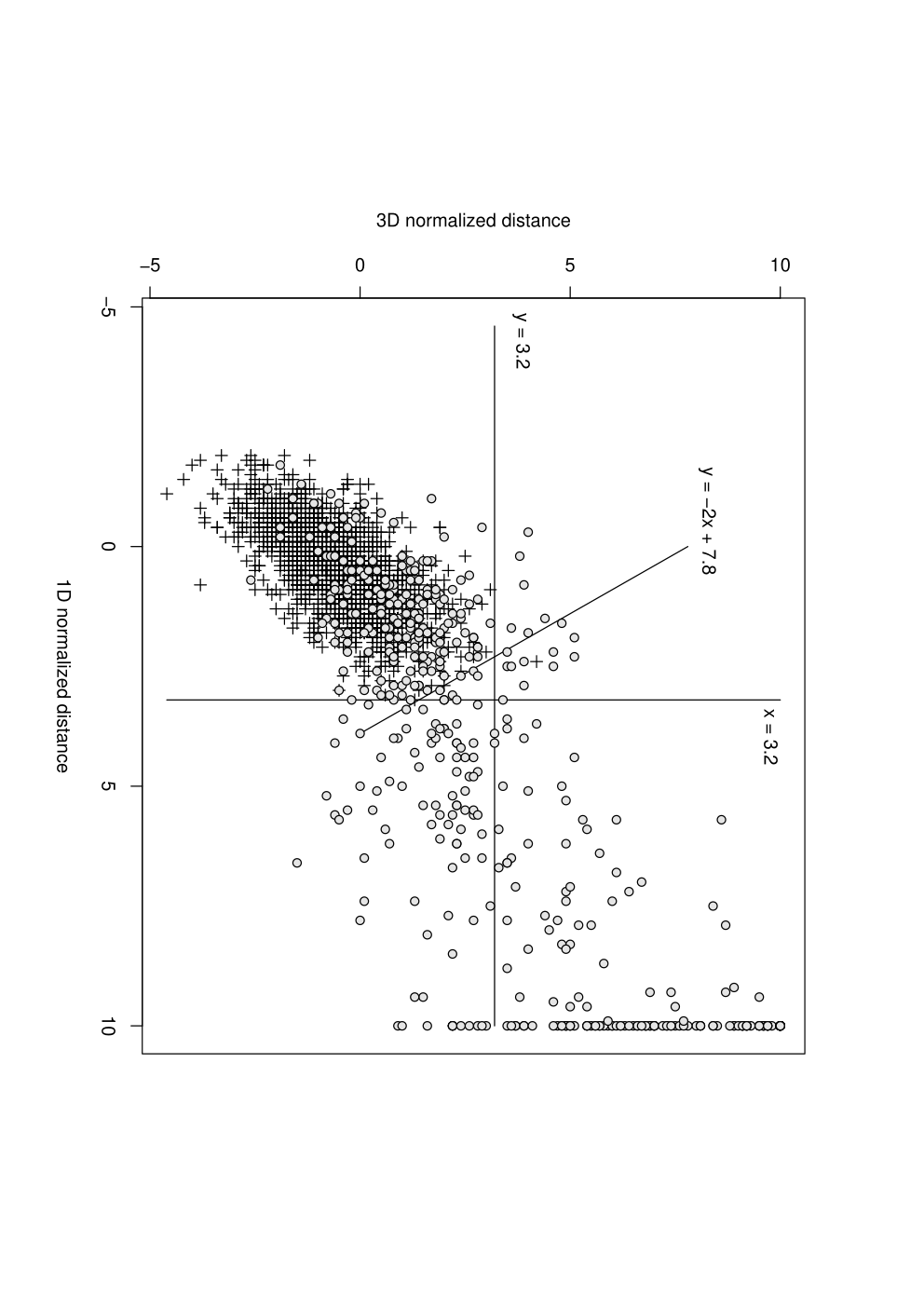
Several score functions, other than the ones described in section 2.2, can be developed. The only point that matters is whether these functions are local or non-local. The same sieve principle as the one described for the two above score functions is still applicable. The difference is that now the resulting cores are characterized by a number of scores greater than two. This makes the visual inspection as explained above difficult and one must rely, for instance, on a Support Vector Machine (SVM) algorithm to find the hyperplanes that separate positive from negative cases.
3 FROST: a computer science vision
3.1 Formal definition
In this section we give a more formal definition of protein threading problem (PTP) and simultaneously introduce some existing terminology. Our definition is very close to the one given in [9, 34]. It follows a few basic assumptions widely adopted by the protein threading community [11, 35, 9, 34, 12, 17]. Consequently, the algorithms presented in the next sections can be easily plugged in most of the existing fold recognition methods based on threading.
Query sequence
A query sequence is a string of length over the 20-letter amino acid alphabet. This is the amino acid sequence of a protein of unknown structure which must be aligned with core templates from the database.
Core template
All current threading methods replace the 3D coordinates of the known structure by an abstract template description in terms of core blocks or segments, neighbor relationships, distances, environments, as explained in section 2.2. This avoids the computational cost of atomic-level mechanics in favor of a more abstract, discrete representation of alignments between sequences and cores.
We consider that a core template is an ordered set of segments or blocks. Segment has a fixed length of amino acids. Adjacent segments are connected by variable length regions, called loops (see Fig. 3(a)).

(a)

(b)

(c)
Segments usually correspond to the most conserved parts of secondary structure elements (-helices and -strands). They trace the path of the conserved fold. Loops are not considered as part of the conserved fold and consequently, the pairwise interactions between amino acids belonging to loops are ignored. It is generally believed that the contribution of such interactions is relatively insignificant. The pairwise interactions between amino acids belonging to segments are represented by the so-called contact map graph (see Fig. 3(b)). Different definitions for residues in contact in the core can be used, for instance in [12] they assume that two amino acids interact if the distance between their atoms is within Å and they are at least positions apart along the template sequence (with and ). There is an interaction between two segments, and , if there is at least one pairwise interaction between amino acids belonging to and amino acids belonging to . Let be the set of segment interactions. The graph with vertices and edges is called generalized contact map graph (see Fig. 3(c)).
Alignments
Let us note, first, that in this section we adopt an inverse perspective and describe the alignment of a sequence onto a core as positioning the segments along the sequence. The problem remains exactly the same but it is easier to describe this way. Such an alignment is called feasible if the segments preserve their original order and do not overlap (see Fig 4(a)).

(a)
| abs. position | 1 | 2 | 3 | 4 | 5 | 6 | 7 | 8 | 9 | 10 | 11 | 12 | 13 | 14 | 15 | 16 | 17 | 18 | 19 | 20 |
|---|---|---|---|---|---|---|---|---|---|---|---|---|---|---|---|---|---|---|---|---|
| rel. position block 1 | 1 | 2 | 3 | 4 | 5 | 6 | 7 | 8 | 9 | |||||||||||
| rel. position block 2 | 1 | 2 | 3 | 4 | 5 | 6 | 7 | 8 | 9 | |||||||||||
| rel. position block 3 | 1 | 2 | 3 | 4 | 5 | 6 | 7 | 8 | 9 |
(b)
An alignment is completely determined by the starting positions of all segments along the sequence. In fact, rather than absolute positions, it is more convenient to use relative positions. If segment starts at the th query sequence character, its relative position is . In this way the possible (relative) positions of each segment vary between 1 and (see Fig. 4(b)). The set of feasible alignments is
| (3) |
The number of possible alignments (the search space size of PTP) is , which is a huge number even for small instances (for example, if and then ).
Most of the alignment methods impose an additional feasibility condition, upper and lower bounds on the lengths of query zones not covered by segments (loops). This condition can be easily incorporated by a slight modification in the definition of relative segment position.
In the above definition, gaps are not allowed within segments. They are confined to loops. As explained above, the biological justification is that segments are conserved so that the probability of insertion or deletion within them is very small.
3.2 Network flow formulation
This section follows the formulation proposed in [27, 10]. In order to develop appropriate mathematical models, PTP is restated as a network optimization problem. Let be a digraph with vertex set and arc set . The vertex set is organized in columns, corresponding to segments from the aligned core. In each column, each vertex correspond to a relative position of the corresponding segment along the sequence. Then with the number of segments and the number of relative positions (see Fig. 5 where and ). A cost is associated to each vertex as defined by the scoring function (1). The arc set is divided into two subsets : is a subset containing arcs between adjacent segments and contains arcs between remote segments. Thus with
To each arc is associated a cost as defined by the scoring function (2). The arcs from will be referred as -arcs and the arcs from as -arcs.

By adding two extra vertices and and the corresponding arcs , and , , (considered as -arcs) one can see the one-to-one correspondence between the set of the feasible threadings and the set of the S-T path on -arcs in . We say that a S-T path activates its vertices and -arcs. A -arc is activated by a S-T path if both ends are on the path. We call the subgraph induced by the -arcs of an S-T path and the activated -arcs augmented path. Then PTP is equivalent to finding the shortest augmented path in . Fig. 5 illustrates this correspondence.
3.3 Integer programming formulation
Let be binary variables associated with vertices in the previous network. Then is one if segment is at position and zero otherwise (vertex is activated or not). Let be the polytope defined by the following constraints :
| (4) | ||||||
| (5) | ||||||
| (6) |
Constraint (4) ensures that each block is assigned to exactly one position. Constraint (5) describes a non-decreasing path in the alignment graph. These constraints are illustrated in Fig6.

In order to take into account the interaction costs, we introduce a second set of variables , with and . These variables correspond to -arcs and -arcs in the network flow formulation. For the sake of readability, we will use the notation for with the arc set. The variable is set to one if the corresponding arc is activated.
Then, we define the following constraints :
| (7) | ||||||
| (8) | ||||||
| (9) |
These constraints ensure that setting variables and to one (the path passes through these two points), activates the arc . Finding the shortest augmented path in graph (i.e. solving PTP) is then equivalent to minimize the following function subject to the previous constraints :
| (10) |
This model, introduced in [11], is known as MYZ model. It significantly outperforms the MIP model used in the RAPTOR package [12] for all large instances (see [11] for more details). Both models (MYZ and RAPTOR) are solved using a linear programming relaxation (LP). The advantage of these models is that their LP relaxations give the optimal solution for most of the real-life instances. They have significantly beter performance than the branch & bounds approach proposed in [9]. Their drawback is their huge size (both number of variables and number of constraints) which makes even solving the LP relaxation slow. In the next section we present more efficient approaches for solving these models. They are based on Lagrangian relaxation.
3.4 Lagrangian approaches
Consider an integer program
| (11) |
Relaxation and duality are the two main ways of determining and upper bounds for . The linear programming relaxation is obtained by changing the constraint in the definition of by . The Lagrangian relaxation is very convenient for problems where the constraints can be partitioned into a set of “simple” ones and a set of “complicated” ones. Let us assume for example that the complicated constraints are given by , where is matrix, while the simple constraints are given by . Then for any the problem
where is the Lagrangian relaxation of (11), i.e. for each . The best bound can be obtained by solving the Lagrangian dual . It is well known that the relation holds.
3.5 Lagrangian relaxation
We show now how to apply Lagrangian relaxation (LR) taking Eq. (8) as a complicated constraint. Recall that this constraint insures that the -variables and the -variables select the same position of segment . By relaxing such a constraint, we relax the right end of a z-arcs. This means that an arc can be activated even though its right end is not on the path, as it is illustrated in Fig7(a). For a fixed , the relaxed augmented path problem obtained in this way can be solved in a polynomial time using a dynamic programming (see [36]).

(a)

(b)
In order to find the Lagrangian dual one has to look for the maximum of a concave piecewise linear function. This appeals for using the so called sub-gradient optimization technique. For the function , the vector , where is an optimal solution to , is a sub-gradient at . The following sub-gradient algorithm is an analog of the steepest ascent method for maximizing a function:
- •
(Initialization): Choose a starting point , and . Set and find a sub-gradient .
- •
While and do { , ; find }
This algorithm stops either when , (in which case is an optimal solution) or after a fixed number of iterations . The parameter determines the decrease of the sub-gradient step.
Note that for each the solution defined by the -variables is feasible for the original problem. In this way at each iteration of the sub-gradient optimization we have a heuristic solution. At the end of the optimization we have both lower and upper bounds on the optimal objective value.
Symmetrically, we can relax the left end of each link or even relax the left end of one part of the links and the right end of the rest (see figure 7(b)). This approach is used in [14]. The same paper describes a branch-and-bound algorithm using this Lagrangian relaxation instead of the LP relaxation. This is the default algorithm in the FROST package.
Another relaxation, called cost-splitting (CS), is presented in [37]. The results presented in this paper clearly show that CS slightly outperforms LR, and both (LR and CS) relaxations are significantly faster than LP (see Fig. 8). The interested reader can find further details concerning these approaches in [36].

4 Dividing FROST into modules for distribution over a cluster
The following two sections are based on the results presented in [38].
4.1 Amount of computation to be done
In section 2.5 we described the FROST functioning. From a
computational viewpoint, this procedure can be divided into 2 phases:
the first one is the computation of score distributions (hereafter
called phase ) and the second one is the alignment of the sequence
of interest with the dataset of templates (hereafter called phase
for evaluation) making use of the previously calculated distributions.
These two phases are repeated for each filter (1D and 3D). We denote
by Ali1D(Q,C) the process of aligning a query sequence (Q) with
a core (C) in the 1D filter and by Ali3D(Q,C) the more computer
intensive alignment process of the 3D filter. Although we have a very
efficient implementation of the corresponding algorithm based on a
Lagrangian relaxation technique, computing the score distributions for
all the templates takes more than a month when performed sequentially.
The whole procedure requires the following computations:
- 1.
Phase : align non homologous sequences in order to obtain the scores distributions for all templates and all filters. Since five distributions are associated to any template, and there are about 200 sequences for each distribution, this procedure needs solving about 1,200,000 quadratic problems
Ali1Dand the same amount of NP-complete problemsAli3D. - 2.
Phase : align the query with the dataset of templates which requires solving several hundreds of quadratic problems
Ali1Dand NP-complete problemsAli3D(where is usually ten).
Figure 9 shows the distribution of the alignment problems needed to be solved during phase and gives an idea of the amount of computation required by the 3D filter. The number of the problems is about 1,200,000 while the size of the largest instance is .

Figure 10 shows the plot of the mean CPU time required to solve the 3D problems involved in phase as a function of the number of possible alignments88 8 The mean CPU time here concerns macro-tasks each one containing ten (gran3D=10) instances Ali3D of the same size (see section 4.3).

The purpose of the procedure proposed in the next section is to distribute all these tasks.
Note that phase needs to be repeated each time the fitness functions or the library of templates change, which is a frequent case when the program is used in a development phase.
4.2 Distribution of the computations: dividing FROST into modules
The first improvement in the distributed version (DFROST) compared to the original FROST consists in clearly identifying the different stages and operations in order to make the entire procedure modular. The process of computing the scores distributions is dissociated from the alignment of the query versus the set of templates. We therefore split the two phases ( and ) which used to be interwoven in the original implementation. Such a decomposition presents several advantages.
Some of them are:
- •
Phase is completely independent from the query, it can be performed as a preprocessing stage when it is convenient for the program designer.
- •
The utilization of the program is simplified. Note that only the program designer is supposed to execute phase , while phase is executed by an “ordinary” user. From a user’s standpoint DFROST is significantly faster than FROST, since only phase is executed at his request (phase being performed as a preprocessing step).
- •
The program designer can easily carry out different operations needed for further developments of the algorithm or for database updating such as: adding new filters, changing the fitness functions, adding a new template to the library, etc.
- •
This organization of DFROST in modules is very suitable for its decomposition in independent tasks that can be solved in parallel.
The latter point is discussed in details in the next section.
4.3 Parallel Algorithm
We distinguish two kinds of atomic independent tasks in DFROST: the
first is related to solving an instance of a problem of type
Ali1D, while the second is associated with solving an instance
of an Ali3D problem99
9
In reality this problem can be
further decomposed in subtasks. Although non independent, these
subtasks can be executed in parallel as show in
[11, 10]. This parallelization could be easily
integrated in DFROST if necessary..
Hence phase consists in solving 1,200,000 independent tasks of
type Ali1D and Ali3D, while phase consists
in solving several hundreds of independent tasks Ali1D and ten
independent tasks Ali3D. The final decision requires sorting
and analysis of the best solutions of type Ali1D and the
best solutions of type Ali3D.
There is a couple of important observations to keep in mind in order
to obtain an efficient parallel implementation for DFROST. The first
is that the exact number of tasks is not known in advance. Second,
which is even more important, the tasks are irregular (especially
tasks of type Ali3D) with unpredictable and largely
varying execution time. In addition, small tasks need to be aggregated
in macro-tasks in order to reduce data broadcasting overhead. Since
the complexity of the two types of tasks is different, the granularity
for macro-tasks Ali1D should be different from the granularity
for macro-tasks Ali3D.
The parallel algorithm that we propose is based on centralized
dynamic load balancing: macro-tasks are dispatched from a
centralized location (pool) in a dynamic way. The work pool is managed
by a “master” who gives work on demand to idle “slaves”.
Each slave executes the macro-tasks assigned to it by solving
sequentially the corresponding subproblems (either Ali1D or
Ali3D). Note that dynamic load balancing is the only reasonable
task-allocation method when dealing with irregular tasks for which the
amount of work is not known prior to execution.
In phase the pool contains initially several hundreds of tasks of
type Ali1D. The master increases the work granularity by
grouping gran1D of them in macro-tasks. These macro-tasks are
distributed on demand to the slaves that solve the corresponding
problems. The solutions computed in this way are sent back to the
master and sorted by it locally. The templates associated to the
best scores yield problems of type Ali3D. The master groups
them in batches of size gran3D and transmits them to the slaves
where the associated problems are solved. The granularity
gran1D is bigger than the gran3D granularity. Finally
the slaves send back to the master the computed solutions.
The strategy in phase is simpler. The master only aggregates tasks
in macro-tasks of size either gran1D or gran3D, sends
them on demand to idle slaves (where the corresponding problems are
sequentially solved), and finally gathers the distributions that have
been computed. The master processes the library of templates in a
sequential manner. First, it aims at distributing all tasks for a
given template to the slaves. However, when the list of tasks for a
given template becomes empty, but the granularity level is not attained,
the master proceeds to distribute tasks from the next template.
This strategy allows to reduce globally the idle time of the
processors.
5 Computational experiments
5.1 Running times
The numerical results presented in this section (see Table 1) were obtained on a cluster of 12 Intel(R) Xeon(TM) CPU 2.4 GHz, 2 Gb Ram, RedHat 9 Linux, connected by a 1 Gb Ethernet network. The behavior of DFROST was tested by entirely computing the phase D of the package, i.e. all the distributions for 1125 templates for both filters.
| Number of tasks | Wall clock time | Total sequential time | Speed-up | |
|---|---|---|---|---|
| 3D filter | 1,104,074 | 3d 3h 20m | 37d 5h 11m | 11.9 |
| 1D filter | 1,107,973 | 31m | 4h 13m | 8.2 |
| Both filters | 2,202,047 | 3d 3h 51m | 37d 9h 24m | 11.8 |
In the case of 3D filter, solving 1,104,074 alignments in parallel as shown on table 1 is very efficient. Comparison of the total sequential running times with the wall clock time of the master shows that we obtain a speed-up of about 12, i.e., an efficiency close to one. In the case of 1D filter, for solving 1,107,973 alignments, the speed up is lower but then the total sequential time is much shorter than for solving 3D tasks.
These significant results, obtained on such a large data set, justify the work done to distribute FROST and prove the efficiency of the proposed parallel algorithm.
Details from this execution are presented in table 2.
The value of the parameters gran1D and gran3D were experimentally fixed to 1000 and 10 respectively.
| Template | DFROST | CPU tot | Cpu av | NAli |
|---|---|---|---|---|
| 1BGLA0 | 15455 | 107569 | 113 | 945 |
| 1ALO_0 | 9565 | 96579 | 97 | 995 |
| 1CXSA0 | 5988 | 55808 | 58 | 960 |
| 1DIK_0 | 4506 | 46855 | 47 | 977 |
| 1BGW_0 | 4152 | 45286 | 45 | 1000 |
| 1CLC_0 | 3580 | 37973 | 39 | 969 |
| 1AA6_0 | 3357 | 35819 | 38 | 926 |
| 1DJXB0 | 3025 | 31276 | 31 | 1000 |
| 1DAR_0 | 2705 | 28671 | 28 | 1000 |
| 1AOZA0 | 2477 | 25156 | 26 | 935 |
| 1AK5_0 | 2072 | 22326 | 22 | 979 |
| 1AUIA0 | 2016 | 22010 | 22 | 1000 |
| 1AOFB0 | 2065 | 21619 | 21 | 1000 |
| 1BHGA0 | 1904 | 20740 | 21 | 980 |
| 1AORA0 | 1920 | 20059 | 20 | 995 |
| 1AYL_0 | 1807 | 18961 | 19 | 973 |
| 1EUT_0 | 1753 | 18883 | 18 | 995 |
| 1CTN_0 | 1535 | 16670 | 16 | 1000 |
| 1ECL_0 | 1439 | 15589 | 16 | 953 |
| 1ATIA0 | 1492 | 15463 | 15 | 980 |
| 1CIY_0 | 1441 | 15044 | 15 | 1000 |
| 1BYB_0 | 1307 | 13892 | 14 | 990 |
| 1COY_0 | 1204 | 13150 | 13 | 957 |
| 1DLC_0 | 1104 | 11825 | 13 | 907 |
| 1BDP_0 | 1173 | 12814 | 12 | 995 |
| 1AOP_0 | 1134 | 12323 | 12 | 1000 |
| 1AG8A0 | 1120 | 12153 | 12 | 990 |
| 1BMFC0 | 1094 | 11338 | 11 | 1000 |
| 1ECFB0 | 1052 | 11254 | 11 | 990 |
| 1DERA0 | 1047 | 11109 | 11 | 1000 |
| 1ALKA0 | 1022 | 10937 | 11 | 965 |
| 1DPE_0 | 988 | 10626 | 11 | 957 |
| 1DDT_0 | 973 | 10349 | 10 | 1000 |
| 1AC5_0 | 907 | 9877 | 9 | 1000 |
| 1CAE_0 | 913 | 9870 | 9 | 990 |
| 1BMFD0 | 914 | 9467 | 9 | 998 |
| 1DPGA0 | 875 | 9092 | 9 | 1000 |
| 1ASYA0 | 1102 | 8634 | 9 | 952 |
| 1LYLA0 | 782 | 8335 | 8 | 990 |
| 1BIF_0 | 657 | 7129 | 7 | 948 |
| 1AD3A0 | 629 | 6669 | 6 | 1000 |
| 1DNPA0 | 776 | 6580 | 6 | 960 |
We can calculate an upper limit for the number of processors beyond
which it is not any more possible to benefit from adding more
processors. The maximum time for an alignment is 797.4 seconds 3, this
time is the lower limit of the wall clock time for the complete
computation of the distributions for Ali3d. The total CPU time
necessary to calculate all Ali3D alignments is 3,215,460
seconds. Thus, adding more than 4032 processors
(3215460/797.4) will not further accelerate the global process. This
gives a theoretical upper limit. The assumption behind this procedure is that
difficult computations are submitted first. This strategy was not
implemented in the results presented in [38] since it
requires a criterion for a preliminary running time task estimation.
Our observation on the code behavior when computing all distributions
confirm that a meaningful criterion is the solutions search space (see
figure 10). Another criterion could be the observed
in the past running time for a task.
5.2 Statistical analysis of the results
Using this parallel algorithm we were able to compute all
distributions for the entire FROST templates library. This was never
done with the sequential code, because of large templates like 1BGLA0 with
sequences as long as 528 amino acids, leading to a number of possible
alignments as large as 6.647E+77. Statistics concerning the running time distribution are
presented on Figure 11.
On average, the running time distribution of all Ali1D
tasks, is characterized by the following data:
| minimum | 1st quartile | mean | 3rd quartile | maximum |
| 0 s | 0.03 s | 0.58 s | 2.32 s | 797.4 s |
Note that these times correspond to one alignment.


We observed that for 188 templates the computation of the distributions requires more than one hour CPU time. Statistical details concerning the running time of the four most time consuming templates are presented in table 3. Remember, that a PTP instance (i.e. when the query and the 3D structure are fixed) is considered as an atomic independent task in the current parallel strategy. Yet, as shown in [11, 10], such an instance could be further decomposed in subtasks that could be executed in parallel. We studied the need for implementing this parallelization in the package FROST. However, taking in account that: i) the number of independent tasks when computing distributions is very high; ii) the data from tables 2 and 3, as well as their statistical recapitulations in figure 11, clearly showing that really hard PTP instances are rather rare; iii) the speedup reported in section 5 is very satisfactory, we decided, for the time being, to stay with the current parallel strategy.
| Nb Sol | NAli | Min | Med | Mean | Max | |||
|---|---|---|---|---|---|---|---|---|
| 1BGLA0 | 55 | 0.95 | 0.96 | 0.98 | 0.97 | 0.98 | 1.02 | |
| 56 | 0.95 | 0.96 | 0.97 | 0.97 | 0.98 | 1.01 | ||
| 192 | 35.6 | 39.9 | 42.2 | 45.2 | 50.0 | 73.2 | ||
| 199 | 102.4 | 116.3 | 131.0 | 145.7 | 164.6 | 510.0 | ||
| 150 | 203.8 | 229.7 | 252.6 | 291.7 | 327.5 | 797.4 | ||
| 1QBA_0 | 58 | 1.82 | 1.83 | 1.83 | 1.84 | 1.84 | 1.89 | |
| 57 | 1.82 | 1.83 | 1.83 | 1.84 | 1.84 | 1.89 | ||
| 197 | 27.1 | 30.2 | 32.5 | 36.3 | 39.8 | 76.6 | ||
| 200 | 68.4 | 77.5 | 86.9 | 101.4 | 116.0 | 354.8 | ||
| 200 | 130.1 | 154.7 | 178.3 | 207.0 | 239.8 | 789.8 | ||
| 1ALO_0 | 57 | 0.85 | 0.87 | 0.87 | 0.87 | 0.88 | 0.89 | |
| 57 | 0.85 | 0.86 | 0.87 | 0.87 | 0.87 | 0.89 | ||
| 190 | 25.8 | 29.3 | 36.1 | 40.8 | 46.7 | 135.2 | ||
| 200 | 67.4 | 86.3 | 113.2 | 123.2 | 134.8 | 397.6 | ||
| 200 | 139.9 | 175.7 | 231.0 | 262.2 | 303.4 | 735.0 | ||
| 1YGE_0 | 61 | 0.39 | 0.40 | 0.41 | 0.41 | 0.41 | 0.43 | |
| 59 | 0.40 | 0.41 | 0.41 | 0.41 | 0.42 | 0.42 | ||
| 192 | 34.8 | 39.9 | 43.1 | 47.5 | 48.9 | 139.8 | ||
| 173 | 71.2 | 80.5 | 89.5 | 102.0 | 115.9 | 365.1 | ||
| 199 | 120.2 | 138.5 | 158.3 | 178.2 | 208.9 | 443.7 |
6 Future research directions
It is well known that large fractions of the proteins have a modular organization as shown on Figure 12. Such proteins are called multi-domain proteins. These modules can be detected at the level of the amino acid sequence as similar subsequences that are found in different protein sequences. In the 3D structure of the whole proteins these modules correspond, usually to one, sometimes to several, substructures called structural domains1010 10 in the literature the terms domain and module are often used somewhat interchangeably. In this paper we restrict the use of module to subsequences and domain to 3D substructures [40] (see the right hand side of Figure 12).

Several cases can occur when studying such multi-domain proteins. Let us illustrate this point with the PEP-utilizers domain presented on Figure 12.
If one wishes to analyze the PEP-utilizers module family one needs to compare the corresponding sequences over their complete lengths. Using global alignment of the sequences (i.e. gaps before the beginning of a sequence and after its end are penalized) will not give a satisfactory result. If the goal of the study is to search for the PEP-utilizers module in a set of sequences (such as those shown in Fig. 12), one must use a semi-global alignment where the gaps before the beginning, and after the end of a sequence are set to zero. This allows the shorter sequence of the PEP-utilizers module to “slide” along the longer sequences until it finds the best match.
The most general case occurs when, comparing two sequences, for instance the second and the fifth in Fig. 12, one is trying to analyze what is common between these sequences. This corresponds to carrying out a local alignment, that is, finding subsequences in both sequences that have the maximum score when aligned (for a given score function).
The local alignment is the most general alignment technique. Accordingly, this is the convenient alignment when comparing an unknown sequence with a database of sequences, since it is unknown beforehand what the similarity is between the query and the database sequences.
Due to the strong analogy that exists between sequence-sequence alignment methods and sequence-structure alignment methods, the above considerations are also valid, mutatis mutandis, for protein threading methods.
In section 2.4 we mentioned that FROST permits only global alignment of a sequence with a core. Even more, to the best of our knowledge, no current protein threading approach exists, that uses non-local score functions for providing an exact solution, and that is able to carry out semi-global and local alignments. Some ideas to tackle this problem have been presented by G. Collet and al. in [42, 43] where mathematical formulations, based on MIP models for semi-global and local sequence/structure alignment, are discussed. The latest one is also called flexible alignment since it allows omissions of blocks during the alignment process (see Fig. 13).
7,4)
0,3)B11 .2,3)B12 .4,3)B13 .6,3)B14 .8,3)B15 1,3)B16 1.2,3)B17 1.4,3)B18 1.6,3)B19
2,3)B22 2.2,3)B23 2.4,3)B24 2.6,3)B25 2.8,3)B26 3,3)B27 3.2,3)B28
3.6,3)B31 3.8,3)B32 4,3)B33 4.2,3)B34 4.4,3)B35
4.8,3)B41 5,3)B42 5.2,3)B43 5.4,3)B44
5.8,3)B51 6,3)B52 6.2,3)B53 6.4,3)B54 6.6,3)B55 6.8,3)B56
,1)1ptSm7 )1ptSm7 ,1)1ptSm7 ,1)1ptSm7 ,1)1ptSm7 ,1)1ptSm7 )1ptSm7 1)1ptSm6 1)1ptSm5 1)1ptSm4 1)1ptSm3 1ptSm2 )1ptSm1 )1ptS1 )1ptS2 )1ptS3 1ptS4 1)1ptS5 1)1ptS6 1)1ptS7 1)1ptS8 1ptS9 1)1ptS10 1)1ptS11 1)1ptS12 1)1ptS13 1ptS14 1)1ptS15 1)1ptS16 1)1ptS17 1)1ptS18 1ptS19 1)1ptSm1 1)1ptS1 1)1ptS2 1)1ptS3 1ptS4 1)1ptS5 1)1ptS6 1)1ptS7 1)1ptS8 1ptS9 1)1ptS10 1)1ptS11 1)1ptS12 1)1ptS13 1ptS14 1)1ptSm1 1)1ptS1 1)1ptS2 1)1ptS3 1ptS4 1)1ptS5 1)1ptS6 1)1ptS7 1)1ptS8 1ptS9 1)1ptS10
4,1)D11 4.2,1)D12 4.4,1)D13 4.6,1)D14 4.8,1)D15 5,1)D16 5.2,1)D17 5.4,1)D18 5.6,1)D19
6.4,1)D22 6.6,1)D23 6.8,1)D24 7,1)D25 7.2,1)D26 7.4,1)D27 7.6,1)D28
8.4,1)D41 8.6,1)D42 8.8,1)D43 9,1)D44
Semi-global and flexible alignments raise a number of new questions. Performing such alignments necessitates the alignment of cores with potentially very long sequences (the largest proteins known are up to 10 000 residues long). The process of computing distributions (see 2.4) needs to be significantly modified in the context of arbitrarily long sequences. In addition, these types of alignment will drastically increase the solution space and the corresponding running time. In order to manage such an increase of the computational requirements the future semi-global and flexible alignment algorithms will need more and more parallel and distributed computing.
7 Conclusion
Fold recognition (protein threading) is rather typical of problems that occur in bioinformatics. It requires knowledge from different disciplines: biology for the definition of cores, physical-chemistry for the development of score functions, computer science for the conception of efficient alignment algorithms and statistics for explaining the significance of the alignment score.
Sequence comparison methods play an outstanding role for exploiting protein sequence data, in particular for in silico functional analysis. These methods are versatile and extremely efficient as long as close homologs are considered. Fold recognition techniques are intended to replace them when the much more difficult case of remote homologs needs to be tackled. Unfortunately, fold recognition techniques are computer intensive and, for the moment, are less universal. In particular the problem of fold recognition has received a satisfactory solution only for the case of global alignments whereas, due to the protein modularity properties, semi-global and local alignments are urgently needed. Fold recognition methods are also plagued by the lack of a statistical theory permitting to assess the significance of alignment scores. Our goal, in the near future, is to set fold recognition methods on an equal footing with sequence alignment methods in terms of available types of alignment and assessment of the alignment score significance.
Of course, due to the inescapable NP-hard property of fold recognition alignment algorithms, these methods will always be more demanding in terms of computer resources than sequence alignments, although we are able to achieve pruning peak rate as high as per second for global alignments. However, as shown in this paper, it is possible to harness the power of grid computing to perform the heavy calculations that will be needed to analyze the 500 currently sequenced microbial genomes and the further thousand that are to be released next year.
References
- [1] SF Altschul, TL Madden, AA Schaffer, J Zhang, Z Zhang, W Miller, and DJ Lipman. Gapped blast and psi-blast: a new generation of protein database searchprograms. Nucleic Acids Res, 25:3389–402, 1997.
- [2] S.E. Brenner, C. Chothia, and T.J. Hubbard. Assessing sequence comparison methods with reliable structurally identified distant evolutionary relationships. Proc Natl Acad Sci U S A, 95:6073–6078, 1998.
- [3] C. Chothia. One thousand families for the molecular biologist. Nature Biotechnology, 22:1317–1321, 2004.
- [4] CA Orengo, DT Jones, and JM Thornton. Protein superfamilies and domain superfolds. Nature, 372:631–4, 1994.
- [5] F.M. Pearl, C.F. Bennett, J.E. Bray, A.P. Harrison, N. Martin, A. Shepherd, I. Sillitoe, J. Thornton, and C.A. Orengo. The cath database: an extended protein family resource for structural and functional genomics. Nucleic Acids Research, 31(1):452–455, 2003.
- [6] A. Andreeva, D. Howorth, S.E. Brenner, T.J.P. Hubbard, C. Chothia, and A.G. Murzin. Scop database in 2004: refinements integrate structure and sequence family data. Nucleic Acids Research, 32:226–229, 2004.
- [7] A. Marin, J.Pothier, K. Zimmermann, and J-F. Gibrat. Frost: A filter based fold recognition method. Proteins, 49(4):493–509, 2002.
- [8] R.H. Lathrop. The protein threading problem with sequence amino acid interaction preferences is NP-complete. Protein Engineering, 255:1059–1068, 1994.
- [9] R.H. Lathrop and T.F. Smith. Global optimum protein threading with gapped alignment and empirical pair potentials. Journal of Molecular Biology, 255:641–665, 1996.
- [10] N. Yanev and R. Andonov. Parallel divide&conquer approach for the protein threading problem. Concurrency and Computation: Practice and Experience, 16:961–974, 2004.
- [11] R. Andonov, S. Balev, and N. Yanev. Protein threading problem: From mathematical models to parallel implementations. INFORMS Journal on Computing, 16(4):393–405, 2004. Special Issue on Computational Molecular Biology/Bioinformatics, Eds. H. Greenberg, D. Gusfield, Y. Xu, W. Hart, M. Vingro.
- [12] J. Xu, M. Li, G. Lin, D. Kim, and Y. Xu. Raptor: optimal protein threading by linear programming. Journal of Bioinformatics and Computational Biology, 1(1):95–118, 2003.
- [13] Y. Xu and D. Xu. Protein threading using prospect: design and evaluation. Proteins, 40(3):343–354, 2000.
- [14] Stefan Balev. Solving the protein threading problem by lagrangian relaxation. In Jonassen and J. Kim, editors, 4th International Workshop on Algorithms in Bioinformatics, Bergen, Norway. Volume 3240 of LNCS/LNBI WABI 2004, pages 182–193, 2004.
- [15] W.W. Li, R.W. Byrnes, J. Hayes, V.M. Reyes, A. Birnbaum, A. Shahab, C. Mosley, D. Pekurovsky, G.B. Quinn, I.N. Shindyalov, H. Casanova, L. Ang, F. Berman, M.A. Miller, and P.E. Bourne. The encyclopedia of life project: Grid software and deployment. Special Issue on Grid Systems for Life Sciences. New Generation Computing, 2003.
- [16] Thomas Steinke. Alignment & threading on massively parallel computers. Technical report, Berlin Center for Genome Based Bioinformatics, 2003.
- [17] Y. Xu, D. Xu, and E.C. Uberbacher. An efficient computational method for globally optimal threading. Journal of Computational Biology, 5:597–614, 1998.
- [18] SF Altschul. Amino acid substitution matrices from an information theoretic perspective. J Mol Biol, 219:555–65, 1991.
- [19] MO Dayhoff, RM Schwartz, and BC Orcutt. Atlas of protein sequence and structure, volume 5, chapter A model of evolutionary change in proteins, pages 345–352. National Biomedical Research Foundation, Washington DC, 1978.
- [20] S Henikoff and JG Henikoff. Amino acid substitution matrices from protein blocks. Proc Natl Acad Sci U S A, 89:10915–9, 1992.
- [21] SB Needleman and CD Wunsch. A general method applicable to the search for similarities in the aminoacid sequence of two proteins. J Mol Biol, 48, 1970.
- [22] TF Smith and MS Waterman. Identification of common molecular subsequences. J Mol Biol, 147:195–7, 1981.
- [23] WR Pearson. Flexible sequence similarity searching with the fasta3 program package. Methods Mol Biol, 132:185–219, 2000.
- [24] SE Brenner, C Chothia, and TJ Hubbard. Assessing sequence comparison methods with reliable structurallyidentified distant evolutionary relationships. Proc Natl Acad Sci U S A, 95:6073–8, 1998.
- [25] T Madej, JF Gibrat, and SH Bryant. Threading a database of protein cores. Proteins, 23:356–69, 1995.
- [26] T. Akutsu and S. Miyano. On the approximation of protein threading. Theoretical Computer Science, 210:261–275, 1999.
- [27] Nicola Yanev and Rumen Andonov. Solving the protein threading problem in parallel. In IPDPS ’03: Proceedings of the 17th International Symposium on Parallel and Distributed Processing, page 157.1. IEEE Computer Society, 2003.
- [28] J. Xu, M. Li, G. Lin, D. Kim, and Y. Xu. Protein structure prediction by linear programming. In Proceedings of The 7th Pacific Symposium on Biocomputing (PSB), pages 264–275, 2003.
- [29] G. Lancia. Integer programming models for computational biology problems. J. Comput. Sci. & Technol., 19(1):60–77, 2004.
- [30] J. Blazewicz, P. Lukasiak, and M. Milostan. Some operations research methods for analyzing protein sequences and structures. 4OR A Quarterly Journal of Operations Research, 4(2):91–123, 2006.
- [31] S Karlin and SF Altschul. Methods for assessing the statistical significance of molecular sequence features by using general scoring schemes. Proc Natl Acad Sci U S A, 87:2264–8, 1990.
- [32] LA Mirny, AV Finkelstein, and EI Shakhnovich. Statistical significance of protein structure prediction by threading. Proc Natl Acad Sci U S A, 97:9978–83, 2000.
- [33] K. Zimmermann A. Marin, J.Pothier and J-F. Gibrat. Protein structure prediction: bioinformatic approach, chapter Protein threading statistics: an attempt to assess the significance of a fold assignment to a sequence. International University line, 2002.
- [34] J. Setubal and J. Meidanis. Introduction to computational molecular biology. PWS publishing company, 1997.
- [35] R.H. Lathrop, R.G. Rogers Jr., J. Bienkowska, B.K.M. Bryant, L.J. Buturovic, C. Gaitatzes, R. Nambudripad, J.V. White, and T.F. Smith. Computational Methods in Molecular Biology, chapter 12, pages 227–283. Elsevier Science, 1998.
- [36] N. Yanev, P. Veber, R. Andonov, and S. Balev. Lagrangian approaches for a class of matching problems in computational biology. Rapport de recherche RR-5973, INRIA, August 2006. to appear in Computers and Mathematics with Applications, special issue on Computational Biology, Edt.Roberto Tadei.
- [37] P. Veber, N. Yanev, R. Andonov, and V. Poirriez. Optimal protein threading by cost-splitting. In WABI’05 (5th Workshop on Algorithms in Bioinformatics), volume 3692 of Lecture Notes in Computer Science, pages 365–375. Springer, 2005.
- [38] V. Poirriez, R. Andonov, A. Marin, and J-F. Gibrat. Frost: Revisited and distributed. In IPDPS ’05: Proceedings of the 19th IEEE International Parallel and Distributed Processing Symposium (IPDPS’05) - Workshop 7, page 200.1, Washington, DC, USA, 2005. IEEE Computer Society.
- [39] Ross Ihaka and Robert Gentleman. R: A language for data analysis and graphics. Journal of Computational and Graphical Statistics, 5(3):299–314, 1996.
- [40] A.M.Lesk and G.D. Rose. Folding units in globular proteins. PNAS, 78:4304–4308, 1981.
- [41] A. Bateman, L. Coin, R. Durbin, R.D. Finn, V. Hollich, Jones Griffiths, A. Khanna, M. Marshall, S. Moxon, E.L. Sonnhammer, D.J. Studholme, C. Yeats, and S.R. Eddy. The Pfam protein families database. Nucleic Acids Res, 32:D138–41, 2004.
- [42] G. Collet, A. Marin, N. Yanev, R. Andonov, and J-F. Gibrat. Implementing a semi-global alignment algorithm for protein threading methods that use non-local score functions. In Poster of the ROADEF conference, 2006. in French.
- [43] G. Collet, N. Yanev, A. Marin, R. Andonov, and J-F. Gibrat. A flexible model for protein fold recognition. In A. Denise, P. Durrens, S. Robin, E. Rocha, A. de Daruvar, and A. Groppi, editors, Septièmes Journées Ouvertes de Biologie, Informatique et Mathématiques (JOBIM), pages 215–216, 2006.