Spin Networks and Anyonic Topological Computing II
Abstract
We review the -deformed spin network approach to Topological Quantum Field Theory and apply these methods to produce unitary representations of the braid groups that are dense in the unitary groups. The simplest case of these models is the Fibonacci model, itself universal for quantum computation. We here formulate these braid group representations in a form suitable for computation and algebraic work.
keywords
braiding, knotting, linking, spin network, Temperley – Lieb algebra, unitary representation.1 INTRODUCTION
This paper describes the background for topological quantum computing in terms of Temperely – Lieb Recoupling Theory and gives an explicit description of the resulting unitary representations of the Artin braid group, including the Fibonacci model as the simplest case.
We use a recoupling theory that generalizes standard angular momentum recoupling theory, generalizes the Penrose theory of spin networks and is inherently topological. Temperely – Lieb Recoupling Theory is based on the bracket polynomial model for the Jones polynomial. It is built in terms of diagrammatic combinatorial topology. The same structure can be explained in terms of the quantum group, and has relationships with functional integration and Witten’s approach to topological quantum field theory. Nevertheless, the approach given here will be unrelentingly elementary. Elementary, does not necessarily mean simple. In this case an architecture is built from simple beginnings and this archictecture and its recoupling language can be applied to many things including: colored Jones polynomials, Witten–Reshetikhin–Turaev invariants of three manifolds, topological quantum field theory and quantum computing.
The contents of this paper are based upon the work in [10] and we shall refer to results from that paper.
In quantum computing, the application is most interesting because the recoupling theory yields representations of the Artin Braid group into unitary groups . These represententations are dense in the unitary group, and can be used to model quantum computation universally in terms of representations of the braid group. Hence the term: topological quantum computation.
In this paper, we outline the basics of the Temperely – Lieb Recoupling Theory, and show explicitly how unitary representations of the braid group arise from it. We will return to this subject in more detail in subsequent papers. In particular, we do not describe the context of anyonic models for quantum computation in this paper. Rather, we concentrate here on showing how naturally unitary representations of the braid group arise in the context of the Temperely – Lieb Theory. For the reader interested in the relevant background in anyonic topological quantum computing we recommend the following references { [1, 2, 3, 4, 5, 12, 13, 15, 16] }.
Here is a very condensed presentation of how unitary representations of the braid group are constructed via topological quantum field theoretic methods. For simplicity assmue that one has a single (mathematical) particle with label that can interact with itself to produce either itself labeled or itself with the null label When interacts with the result is always When interacts with the result is always One considers process spaces where a row of particles labeled can successively interact, subject to the restriction that the end result is For example the space denotes the space of interactions of three particles labeled The particles are placed in the positions Thus we begin with In a typical sequence of interactions, the first two ’s interact to produce a and the interacts with to produce
In another possibility, the first two ’s interact to produce a and the interacts with to produce
It follows from this analysis that the space of linear combinations of processes is two dimensional. The two processes we have just described can be taken to be the the qubit basis for this space. One obtains a representation of the three strand Artin braid group on by assigning appropriate phase changes to each of the generating processes. One can think of these phases as corresponding to the interchange of the particles labeled and in the association The other operator for this representation corresponds to the interchange of and This interchange is accomplished by a unitary change of basis mapping
If
is the first braiding operator (corresponding to an interchange of the first two particles in the association) then the second operator
is accomplished via the formula where the in this formula acts in the second vector space to apply the phases for the interchange of and
In this scheme, vector spaces corresponding to associated strings of particle interactions are interrelated by recoupling transformations that generalize the mapping indicated above. A full representation of the Artin braid group on each space is defined in terms of the local intechange phase gates and the recoupling transfomations. These gates and transformations have to satisfy a number of identities in order to produce a well-defined representation of the braid group. These identities were discovered originally in relation to topological quantum field theory. In our approach the structure of phase gates and recoupling transformations arise naturally from the structure of the bracket model for the Jones polynomial [6]. Thus we obtain a knot-theoretic basis for topological quantum computing.
2 Spin Networks and Temperley – Lieb Recoupling Theory
In this section we discuss a combinatorial construction for spin networks that generalizes the original construction of Roger Penrose [14]. The result of this generalization is a structure that satisfies all the properties of a graphical as described in our paper on braiding and universal quantum gates [9], and specializes to classical angular momentum recoupling theory in the limit of its basic variable. The construction is based on the properties of the bracket polynomial [7]. A complete description of this theory can be found in the book “Temperley – Lieb Recoupling Theory and Invariants of Three-Manifolds” by Kauffman and Lins [8].
The “-deformed” spin networks that we construct here are based on the bracket polynomial relation. View Figure 1 and Figure 2.
 |
 |
 |
In Figure 1 we indicate how the basic projector (symmetrizer, Jones-Wenzl projector) is constructed on the basis of the bracket polynomial expansion [7]. In this technology, a symmetrizer is a sum of tangles on strands (for a chosen integer ). The tangles are made by summing over braid lifts of permutations in the symmetric group on letters, as indicated in Figure 1. Each elementary braid is then expanded by the bracket polynomial relation, as indicated in Figure 1, so that the resulting sum consists of flat tangles without any crossings (these can be viewed as elements in the Temperley – Lieb algebra). The projectors have the property that the concatenation of a projector with itself is just that projector, and if you tie two lines on the top or the bottom of a projector together, then the evaluation is zero. This general definition of projectors is very useful for this theory. The two-strand projector is shown in Figure 2. Here the formula for that projector is particularly simple. It is the sum of two parallel arcs and two turn-around arcs (with coefficient with is the loop value for the bracket polynomial. Figure 2 also shows the recursion formula for the general projector. This recursion formula is due to Jones and Wenzl and the projector in this form, developed as a sum in the Temperley – Lieb algebra (see Section 5 of this paper), is usually known as the Jones–Wenzl projector.
The projectors are combinatorial analogs of irreducible representations of a group (the original spin nets were based on and these deformed nets are based on the quantum group corresponding to SU(2)). As such the reader can think of them as “particles”. The interactions of these particles are governed by how they can be tied together into three-vertices. See Figure 3. In Figure 3 we show how to tie three projectors, of strands respectively, together to form a three-vertex. In order to accomplish this interaction, we must share lines between them as shown in that Figure so that there are non-negative integers so that This is equivalent to the condition that is even and that the sum of any two of is greater than or equal to the third. For example One can think of the vertex as a possible particle interaction where and interact to produce That is, any two of the legs of the vertex can be regarded as interacting to produce the third leg.
There is a basic orthogonality of three vertices as shown in Figure 4. Here if we tie two three-vertices together so that they form a “bubble” in the middle, then the resulting network with labels and on its free ends is a multiple of an -line (meaning a line with an -projector on it) or zero (if is not equal to ). The multiple is compatible with the results of closing the diagram in the equation of Figure 4 so the the two free ends are identified with one another. On closure, as shown in the Figure, the left hand side of the equation becomes a Theta graph and the right hand side becomes a multiple of a “delta” where denotes the bracket polynomial evaluation of the -strand loop with a projector on it. The denotes the bracket evaluation of a theta graph made from three trivalent vertices and labeled with on its edges.
 |
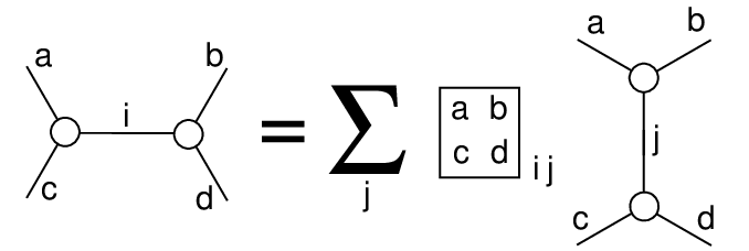
There is a recoupling formula in this theory in the form shown in Figure 5. Here there are “-j symbols”, recoupling coefficients that can be expressed, as shown in Figure 7, in terms of tetrahedral graph evaluations and theta graph evaluations. The tetrahedral graph is shown in Figure 6. One derives the formulas for these coefficients directly from the orthogonality relations for the trivalent vertices by closing the left hand side of the recoupling formula and using orthogonality to evaluate the right hand side. This is illustrated in Figure 7.
 |
 |
 |
Finally, there is the braiding relation, as illustrated in Figure 8.
 |
With the braiding relation in place, this -deformed spin network theory satisfies the pentagon, hexagon and braiding naturality identities needed for a topological quantum field theory. All these identities follow naturally from the basic underlying topological construction of the bracket polynomial. One can apply the theory to many different situations.
2.1 Evaluations
In this section we discuss the structure of the evaluations for and the theta and tetrahedral networks. We refer to [8] for the details behind these formulas. Recall that is the bracket evaluation of the closure of the -strand projector, as illustrated in Figure 4. For the bracket variable one finds that
One sometimes writes the quantum integer
If
where is a positive integer, then
Here the corresponding quantum integer is
Note that is a positive real number for and that
The evaluation of the theta net is expressed in terms of quantum integers by the formula
where
Note that
When the recoupling theory becomes finite with the restriction that only three-vertices (labeled with ) are admissible when All the summations in the formulas for recoupling are restricted to admissible triples of this form.
2.2 Symmetry and Unitarity
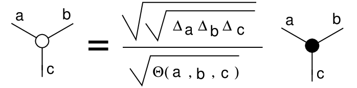
The formula for the recoupling coefficients given in Figure 7 has less symmetry than is actually inherent in the structure of the situation. By multiplying all the vertices by an appropriate factor, we can reconfigure the formulas in this theory so that the revised recoupling transformation is orthogonal, in the sense that its transpose is equal to its inverse. This is a very useful fact. It means that when the resulting matrices are real, then the recoupling transformations are unitary.
Figure 9 illustrates this modification of the three-vertex. Let denote the original -vertex of the Temperley – Lieb recoupling theory. Let denote the modified vertex. Then we have the formula
Lemma. For the bracket evaluation at the root of unity the factor
is real, and can be taken to be a positive real number for admissible (i.e. with ).
Proof. See our basic reference [10].
In [10] we show how this modification of the vertex affects the non-zero term of the orthogonality of trivalent vertices (compare with Figure 4). We refer to this as the “modified bubble identity.” The coefficient in the modified bubble identity is
where form an admissible triple. In particular is even and hence this factor can be taken to be positive real.
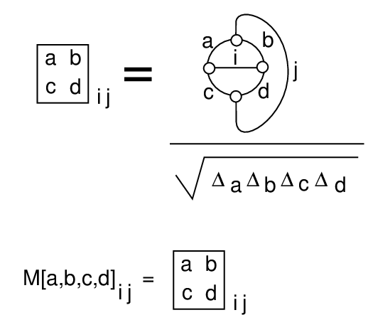
We rewrite the recoupling formula in this new basis and emphasize that the recoupling coefficients can be seen (for fixed external labels ) as a matrix transforming the horizontal “double-” basis to a vertically disposed double- basis. In Figures 10 and 11 we have shown the form of this transformation,using the matrix notation
for the modified recoupling coefficients. In Figure 11 we show an explicit formula for these matrix elements. The proof of this formula follows directly from trivalent–vertex orthogonality (See Figures 4 and 7.), and is given in [10]. The result shown in Figure 11 is the following formula for the recoupling matrix elements.
where is short-hand for the product
In this form, since and are admissible triples, we see that this coeffient can be taken to be positive real, and its value is independent of the choice of and The matrix is real-valued.
It follows from Figure 10 (turn the diagrams by ninety degrees) that
Figure 10 implies the formula
It follows from this formula that
Hence is an orthogonal, real-valued matrix.
 |
 |
 |
Theorem. In the Temperley – Lieb theory we obtain unitary (in fact real orthogonal) recoupling transformations when the bracket variable has the form . Thus we obtain families of unitary representations of the Artin braid group from the recoupling theory at these roots of unity.
Proof. The proof is given by the discussion above and in [10].
3 Explicit Form of the Braid Group Representations
In order to have an explicit form for the representations of the braid group that we have constructed we return to the description of the vector spaces in the introduction to this paper. Here we make this description of the vector spaces more precise as follows. We describe a vector space depending upon a choice of three input and output spins where denotes the possible outcome of two spin labels interacting at a trivalent vertex as in Figure 3. In that figure we see that can represent (the remaining leg of the vertex) and that there is a range of values possible for given by the constraints on and as shown in that figure. Here we insist that the composite interaction shall equal so that the vector space corresponds to the left-hand tree shown in Figure 12. In that figure we indicate the recoupling mapping The matrix form of is composed from the recoupling matrix of Figure 11. In Figure 12 we have labeled corresponding to one of the basis vectors in Similarly, we have corresponding to one of the basis vectors in We let the corresponding vectors be denoted by and respectively. Then we can write
where ranges over the admissible labels for the interaction of and .
 |
To see how the three strand braid group acts on view Figure 13. If we let denote the generator of the three-stand braid group that twists the first two strands and denote the generator that twists the second two strands, then we see that acts directly at a trivalent vertex, giving the formula
where is the braiding factor of Figure 8. On the other hand, we need to perform a recoupling in order to compute the action of As shown in Figure 13, we have
This gives a complete description of the representation of the three-strand braid group on the vector space Our next task is to generalize this to an abitrary “left-associated” tree.
 |
We wish to consider larger left associated trees such as To this purpose it is useful to declare that a fully left-associated product may be written without parentheses. Thus we have
and
Thus we have the recoupling transformation
that will be used for the action of on the space
In the general case we have the spaces with basis elements where has as an outcome, has as an outcome, and so on until has as an outcome. For articulating the braiding we need mappings
The target space has the strands labeled and combined at a vertex so that the braiding for in the target space is local. We also need a basis for This is given by the kets where
We then have
Here it is understood that
where is defined as explained above. Finally, using the recoupling matrix formalism of Figure 10, we have
This completes our description of the action of the braid group on these vector spaces.
3.1 The Fibonacci Model
In the Fibonacci model [11], there is a single non-trivial recoupling matrix
where is the golden ratio and . The local braiding matrix is given by the formula below with
The simplest example of a braid group representation arising from this theory is the representation of the three strand braid group generated by and (Remember that ). The matrices and are both unitary, and they generate a dense subset of supplying the local unitary transformations needed for quantum computing.
 |
In the Fibonacci model there are two labels, as we described in the introduction (see Figure 14): and . can interact with itself to produce either or while acts as an identity element. That is, interacts with to produce only and interacts with to produce Let
The space has basis vectors where runs over all sequences of ’s and ’s without consecutive ’s. The dimension of is the -th Fibonacci number: and
In terms of the matrix , we have and and The representation of the the braid group on is given by the formulas below (with and and the matrix indices for are and corresponding to and respectively). We use the matrix below.
and for
if or
if
These formulas make it possible to do full-scale computer experiments with the Fibonacci model and the generalizations of it that we have discussed. We will pursue this course in a subsequent paper. This model is universal for quantum computation.
ACKNOWLEDGMENTS
The first author thanks the National Science Foundation for support of this research under NSF Grant DMS-0245588.
References
- [1] M. Freedman, A magnetic model with a possible Chern-Simons phase, quant-ph/0110060v1 9 Oct 2001, (2001), preprint
- [2] M. Freedman, Topological Views on Computational Complexity, Documenta Mathematica - Extra Volume ICM, 1998, pp. 453–464.
- [3] M. Freedman, M. Larsen, and Z. Wang, A modular functor which is universal for quantum computation, quant-ph/0001108v2, 1 Feb 2000.
- [4] M. H. Freedman, A. Kitaev, Z. Wang, Simulation of topological field theories by quantum computers, Commun. Math. Phys., 227, 587-603 (2002), quant-ph/0001071.
- [5] M. Freedman, Quantum computation and the localization of modular functors, quant-ph/0003128.
- [6] V.F.R. Jones, A polynomial invariant for links via von Neumann algebras, Bull. Amer. Math. Soc. 129 (1985), 103–112.
- [7] L.H. Kauffman, State models and the Jones polynomial, Topology 26 (1987), 395–407.
- [8] L.H. Kauffman, Temperley – Lieb Recoupling Theory and Invariants of Three-Manifolds, Princeton University Press, Annals Studies 114 (1994).
- [9] L. H. Kauffman and S. J. Lomonaco Jr., Braiding Operators are Universal Quantum Gates, New Journal of Physics 6 (2004) 134, pp. 1-39.
- [10] L. H. Kauffman and S. J. Lomonaco Jr., Spin Networks and anyonic topological computing, In “Quantum Information and Quantum Computation IV”, (Proceedings of Spie, April 17-19,2006) edited by E.J. Donkor, A.R. Pirich and H.E. Brandt, Volume 6244, Intl Soc. Opt. Eng., pp. 62440Y-1 to 62440Y-12.
- [11] L. H. Kauffman and S. J. Lomonaco Jr., - Deformed Spin Networks, Knot Polynomials and Anyonic Topological Quantum Computation, (to appear in JKTR).
- [12] A. Kitaev, Anyons in an exactly solved model and beyond, arXiv.cond-mat/0506438 v1 17 June 2005.
- [13] A. Marzuoli and M. Rasetti, Spin network quantum simulator, Physics Letters A 306 (2002) 79–87.
- [14] R. Penrose, Angular momentum: An approach to Combinatorial Spacetime, In Quantum Theory and Beyond, edited by T. Bastin, Cambridge University Press (1969).
- [15] J. Preskill, Topological computing for beginners, (slide presentation), Lecture Notes for Chapter 9 - Physics 219 - Quantum Computation. http://www.iqi.caltech.edu/ preskill/ph219
- [16] F. Wilczek, Fractional Statistics and Anyon Superconductivity, World Scientific Publishing Company (1990).