Solving Linearized Equations of the $N$ -body Problem Using the Lie-integration MethodSolving Linearized Equations of the $N$ -body Problem Using the Lie-integration Method–D2007

András Pál Thanks: E-mail: apal@szofi.elte.hu (AP); a.suli@astro.elte.hu (ÁS) Affiliation: Department of Astronomy, Loránd Eötvös University, Pázmány Péter sétány 1/A, Budapest H-1117, Hungary Áron Süli Affiliation: Department of Astronomy, Loránd Eötvös University, Pázmány Péter sétány 1/A, Budapest H-1117, Hungary

Accepted 2007 July 18. Received 2007 July 13; in original form 2007 May 25

Abstract

Several integration schemes exits to solve the equations of motion of the $N$ -body problem. The Lie-integration method is based on the idea to solve ordinary differential equations with Lie-series. In the 1980s this method was applied for the $N$ -body problem by giving the recurrence formula for the calculation of the Lie-terms. The aim of this works is to present the recurrence formulae for the linearized equations of motion of $N$ -body systems. We prove a lemma which greatly simplifies the derivation of the recurrence formulae for the linearized equations if the recurrence formulae for the equations of motions are known. The Lie-integrator is compared with other well-known methods. The optimal step size and order of the Lie-integrator are calculated. It is shown that a fine-tuned Lie-integrator can be 30%-40% faster than other integration methods.

Keywords:

celestial mechanics – methods: numerical – methods:

N

-body simulations

1 Introduction

The classical problems of celestial mechanics are described by a system of ordinary differential equations (ODEs). The investigation of the motions in the Solar System, exoplanetary systems, satellites around the Earth or other celestial objects are based on the solutions of such ODEs. However, several modern analysis, including many chaos detection methods require to solve the linearized equations of the problem.

The integration method based on the Lie-series (Gröbner & Knapp 1967) is widely used in celestial mechanics to solve ODEs (see Hanslmeier & Dvorak 1984, hereafter H&D and articles referring to it). The basis of this method is to generate the coefficients of the Taylor expansion of the solution by using recurrence relations. The principal application, i.e. the integration of the $N$ -body problem is described in details in H&D.

1.1 Lie-integration

Here we summarize the key points of this method of numerical integration, using almost identical notations as used by Hanslmeier & Dvorak 1984.

Let us write the differential equation to be solved as

\dot{x}_{i}=f_{i}(\mathbf{x}),

(1)

where $\mathbf{x}\equiv(x_{1},\dots,x_{N})$ is an $\mathbb{R}\to\mathbb{R}^{N}$ and $\mathbf{f}\equiv(f_{1},\dots,f_{N})$ is an $\mathbb{R}^{N}\to\mathbb{R}^{N}$ continuous function and $N$ is the dimension of the vector $\mathbf{x}$ and the vector space where $\mathbf{f}$ maps from and maps to. Let us introduce the differential operator

D_{i}:=\frac{\partial}{\partial x_{i}},

(2)

and the derivation

L_{0}:=\sum\limits_{i=1}^{N}f_{i}\frac{\partial}{\partial x_{i}},

(3)

which is known as the Lie-derivation or Lie-operator. $L_{0}$ is a linear differential operator and one can apply Leibniz’s rule,

L_{0}(ab)=aL_{0}(b)+bL_{0}(a),

(4)

where $a$ and $b$ are $\mathbb{R}^{N}\to\mathbb{R}^{N}$ differentiable functions. It can easily be proven that the solution of equation (1) at a given instance $t+\Delta t$ is formally

\mathbf{x}(t+\Delta t)=\exp\left(\Delta t\cdot L_{0}\right)\mathbf{x}(t),

(5)

where

\exp\left(\Delta t\cdot L_{0}\right)=\sum\limits_{k=0}^{\infty}\frac{\Delta t^{k}}{k!}L_{0}^{k}=\sum\limits_{k=0}^{\infty}\frac{\Delta t^{k}}{k!}\left(\sum\limits_{i=1}^{N}f_{i}D_{i}\right)^{k}.

(6)

The method of Lie-integration is finite approximation of the sum in the right-hand side of equation (6), up to the order of $M$ , namely

\mathbf{x}(t+\Delta t)\approx\left(\sum\limits_{k=0}^{M}\frac{\Delta t^{k}}{k!}L_{0}^{k}\right)\mathbf{x}(t)=\sum\limits_{k=0}^{M}\frac{\Delta t^{k}}{k!}\left(L_{0}^{k}\mathbf{x}(t)\right).

(7)

The proof of equation (5) and other related properties of the Lie-derivation can be found in Gröbner & Knapp 1967 or Hanslmeier & Dvorak 1984.

In spite of the fact that the Lie-derivatives can analytically be calculated up to arbitrary order, the formulae yielded by these expansions are highly complicated even if all kinds of new variables are introduced (see e.g. equations (19d) or (19e) in H&D at page 204). A definitely more efficient way to evaluate the Lie-derivatives is to find a set of recurrence relations. These relations allow us to express the $(n+1)$ th Lie-derivative, e.g. $L^{n+1}\mathbf{x}$ as the function of the derivatives with lower order, namely $L^{j}\mathbf{x}$ where $0\leq j\leq n$ . The initialization of such a recurrence relation is evident, because $L^{0}\mathbf{x}\equiv\mathbf{x}$ . We note that in several applications, well-chosen auxiliary variables have to be introduced to gain a compact set of recurrence relations which can efficiently be evaluated.

1.2 The importance of linearized equations

Wide range of problems related to celestial mechanics require to solve simultaneously the linearized form of the original equations too. The numerous experiments conducted in the last decades show that chaotic behaviour is typical and already occurs in simple but nonlinear systems. This finding throws completely new light upon these systems and the study of chaotic behaviour became of high concern. A major part of the frontline research focuses on the structure of the phase space, therefore the problem to separate ordered and chaotic motion in systems, which posses only a few degrees of freedom and are described by ODEs, has become a fundamental task in a wide area of modern research. The phase space of these nonlinear systems can not be described by the known mathematical tools. To map the phase space and study the chaotic behaviour of a given system fast and reliable numerical tools are needed. These tools are extremely useful in those cases when the inspected dynamical system has more than two degrees of freedom and accordingly its phase space cannot be explored in a direct way or the classical method of surface of section (SoS) can not be applied which is widely used in the case of conservative systems with two degrees and freedom. The basic idea of the method of SoS was invented by Poincaré 1899 and its application was renewed by Hénon & Heiles 1964.

The mathematical foundation of the theory of Lyapunov Characteristic Exponents (LCEs) is approximately of the same age as the SoS and arose progressively in the literature. The use of such exponents dates back to Lyapunov 1907, but was first applied by Oseledec 1968 to characterize trajectories. Hénon & Heiles 1964 found that in an integrable region of the phase space of a dynamical system nearby orbits diverge linearly whereas in a chaotic region they diverge exponentially. The LCEs express these facts in a precise form and many papers were devoted to the application of LCEs in several nonlinear problems.

Unfortunately both methods have a serious drawback. To compute the LCEs the equations have to integrate for infinity, which is numerically impossible. The method of SoS becomes hard to handle and greatly deceiving for systems with more than two degrees of freedom. To overcome these problems was the main motivation in the 1980s that initiated the research to develop new numerical methods to characterize the stochasticity of the trajectories in the phase space in short time-span and in arbitrary dimension. The developed methods can be classified in two groups: one group consists of the methods which are based on the analysis of the orbits, (e.g. SoS or frequency analysis, see Laskar 1990), the other one is based on the time evolution of the tangent vector, i.e. the solution of the linearized equations of motion (e.g. LCE). There are complete software packages designed to analyse systems of celestial mechanics, both for for general integration of motion (Chambers 1999, e.g. Mercury6, see) and for solving linearized equations and calculating LCEs (Milani & Nobili 1988, ORBIT9, see). We also have to mention that there are several improved chaos detection methods which are based on the solution of the linearized equations. Instead of a complete review, we only mention two of them: the method of Fast Lyapunov Indicators (Froeschlé et al. 1997, FLIs, see) and the method of Mean Exponential Growth of Nearby Orbits (Cincotta & Simó 2000; Godźiewski et al. 2001, MEGNO, see).

The aim of this paper is to present a lemma which advances the derivation of the same kind of recurrence relations for the linearized equations. We present these relations for certain classical dynamic systems: for the general $N$ -body problem and for the $N$ -body problem in the reference frame of one of the bodies. In the last section we compare the efficiency of this method with well-known other ones.

2 Linearized equations

The chaos indicators mentioned in the previous section can be obtained if the linearized form of the equations of motion is solved. The solution of the linearized equations is an $\mathbf{\xi}\equiv(\xi_{1},\dots,\xi_{N}):\mathbb{R}\to\mathbb{R}^{N}$ function having the same dimension as the equations of motion has. The linearized equations of equation (1) (any ODE can be written in this form) can be written as

\dot{\xi}_{i}=\sum\limits_{m=1}^{N}\xi_{m}\frac{\partial f_{i}(\mathbf{x})}{\partial x_{m}},

(8)

where the variables $\xi_{i}\equiv\xi_{i}(t):\mathbb{R}\to\mathbb{R}$ are the so-called linearized variables and $\mathbf{x}\equiv\mathbf{x}(t)$ is the solution of equation (1). Equation (8) is linear in $\mathbf{\xi}$ , therefore if $\xi^{(1)}_{i}(t)$ and $\xi^{(2)}_{i}(t)$ are two independent solutions, then $\alpha\xi^{(1)}_{i}(t)+\beta\xi^{(2)}_{i}(t)$ is also a solution. Using the Einstein summation convention equation (8) can be written in a more compact form:

\dot{\xi}_{i}=\xi_{m}D_{m}f_{i}.

(9)

2.1 Lie-derivatives of the linearized equations

Introducing the differential operator

\partial_{i}:=\frac{\partial}{\partial\xi_{i}},

(10)

the coupled system of equations (both the original and the linearized) is

	$\displaystyle\dot{x}_{i}$	$\displaystyle=$	$\displaystyle f_{i},$		(11)
	$\displaystyle\dot{\xi}_{i}$	$\displaystyle=$	$\displaystyle\xi_{m}D_{m}f_{i},$		(12)

and the Lie-operator of equations (11)-(12) is

L=L_{0}+L_{\ell}=f_{i}D_{i}+\xi_{m}D_{m}f_{i}\partial_{i}.

(13)

Lemma

Using the same notations as above the Lie-derivatives of $\xi_{k}$ can be written as

L^{n}\xi_{k}=\xi_{m}D_{m}L^{n}x_{k}=\xi_{m}D_{m}L_{0}^{n}x_{k}.

(14)

Proof

Obviously, equation (14) is true for $n=0$ :

D_{m}L^{0}x_{k}=D_{m}x_{k}=\delta_{mk},

(15)

hence

\xi_{m}D_{m}L^{0}x_{k}=\xi_{m}\delta_{mk}=\xi_{k}.

(16)

Let us suppose that it is true for all $0\leq j\leq n$ and calculate the $(n+1)$ th Lie-derivative of $\xi_{k}$ :

$\displaystyle L^{n+1}\xi_{k}$	$\displaystyle=$	$\displaystyle L\left(\xi_{m}D_{m}L^{n}x_{k}\right)=$	(17)
	$\displaystyle=$	$\displaystyle\left(f_{i}D_{i}+\xi_{j}D_{j}f_{i}\partial_{i}\right)\left(\xi_{m}D_{m}L^{n}x_{k}\right)=$
	$\displaystyle=$	$\displaystyle f_{i}D_{i}\xi_{m}D_{m}L^{n}x_{k}+$
		$\displaystyle+\xi_{j}(D_{j}f_{i})[\delta_{im}D_{m}L^{n}x_{k}+$
		$\displaystyle+\xi_{m}D_{m}\partial_{i}L^{n}x_{k}].$

Here the term $\xi_{m}D_{m}\partial_{i}L^{n}x_{k}$ equals to zero, because $x_{k}$ and $L^{n}x_{k}$ for all $n\geq 0$ do not depend on $\xi$ . Therefore,

$\displaystyle L^{n+1}\xi_{k}$	$\displaystyle=$	$\displaystyle f_{i}D_{i}\xi_{m}D_{m}L^{n}x_{k}+\xi_{j}(D_{j}f_{i})D_{i}L^{n}x_{k}=$	(18)
	$\displaystyle=$	$\displaystyle\xi_{m}f_{i}D_{m}D_{i}L^{n}x_{k}+\xi_{m}(D_{m}f_{i})(D_{i}L^{n}x_{k})=$
	$\displaystyle=$	$\displaystyle\xi_{m}\left(f_{i}D_{m}+D_{m}f_{i}\right)(D_{i}L^{n}x_{k})=$
	$\displaystyle=$	$\displaystyle\xi_{m}D_{m}(f_{i}D_{i})(L^{n}x_{k})=$
	$\displaystyle=$	$\displaystyle\xi_{m}D_{m}L(L^{n}x_{k})=\xi_{m}D_{m}L^{n+1}x_{k}$
	$\displaystyle=$	$\displaystyle\xi_{m}D_{m}L_{0}^{n+1}x_{k}.$

We have applied Young’s theorem, namely

D_{m}D_{i}=D_{i}D_{m},

(19)

and Leibniz rule,

	$\displaystyle D_{m}(f_{i}D_{i})X$	$\displaystyle=$	$\displaystyle D_{m}f_{i}(D_{i}X)=$		(20)
		$\displaystyle=$	$\displaystyle f_{i}(D_{m}D_{i}X)+(D_{m}f_{i})(D_{i}X),$		(20)

where $X$ can be an arbitrary function of $\mathbf{x}$ , in equation (18) $X\equiv L^{n}x_{k}$ . Therefore equation (18) is the same relation for $n+1$ , as equation (14) for $n$ . Continuing the scheme described above, equation (14) can be proven for all positive integer values of $n$ . $\blacksquare$

2.2 An example: applying to the Hénon-Heiles system

Demonstrating the power of the lemma proven in the previous subsection we derive the recurrence relations for the equation of the Hénon-Heiles dynamical system and its linearized form. The Hénon-Heiles system is one of the simplest Hamiltonian systems which shows chaotic behaviour under certain initial conditions (Hénon & Heiles 1964, see).

The equations of motion are derived from the Hamiltonian function

	$\displaystyle H(x,y;v,w)$	$\displaystyle=$	$\displaystyle\frac{1}{2}\left(x^{2}+y^{2}+2x^{2}y-\frac{2}{3}y^{3}\right)+$		(21)
			$\displaystyle+\frac{1}{2}\left(v^{2}+w^{2}\right),$		(21)

where $\dot{x}=v$ and $\dot{y}=w$ . The equations of motion are

$\displaystyle\dot{x}$	$\displaystyle=$	$\displaystyle v,$	(22)
$\displaystyle\dot{y}$	$\displaystyle=$	$\displaystyle w,$	(23)
$\displaystyle\dot{v}$	$\displaystyle=$	$\displaystyle-x-2xy,$	(24)
$\displaystyle\dot{w}$	$\displaystyle=$	$\displaystyle-y-x^{2}+y^{2},$	(25)

and the Lie-operator of this system of equations is

L_{0}=v\partial_{x}+w\partial_{y}+(-x-2xy)\partial_{v}+(-y-x^{2}+y^{2})\partial_{w},

(26)

according to equation (3). It can easily be shown that the recurrence relations of the equations (22) - (25) are the following,

$\displaystyle L_{0}^{n+1}x$	$\displaystyle=$	$\displaystyle L_{0}^{n}v,$	(27)
$\displaystyle L_{0}^{n+1}y$	$\displaystyle=$	$\displaystyle L_{0}^{n}w,$	(28)
$\displaystyle L_{0}^{n+1}v$	$\displaystyle=$	$\displaystyle-L_{0}^{n}x-2\sum\limits_{k=0}^{n}{n\choose k}L_{0}^{k}xL_{0}^{n-k}y,$	(29)
$\displaystyle L_{0}^{n+1}w$	$\displaystyle=$	$\displaystyle-L_{0}^{n}y-\sum\limits_{k=0}^{n}{n\choose k}\left(L_{0}^{k}xL_{0}^{n-k}x-\right.$	(30)
		$\displaystyle\left.-L_{0}^{k}yL_{0}^{n-k}y\right).$	(30)

Let us denote the linearized variables related to $x$ , $y$ , $v$ and $w$ by $\xi$ , $\eta$ , $\phi$ and $\rho$ , respectively. According to equation (14) the Lie-derivatives of these variables are

$\displaystyle L^{n}\xi$	$\displaystyle=$	$\displaystyle\xi_{m}D_{m}L^{n}x,$	(31)
$\displaystyle L^{n}\eta$	$\displaystyle=$	$\displaystyle\xi_{m}D_{m}L^{n}y,$	(32)
$\displaystyle L^{n}\phi$	$\displaystyle=$	$\displaystyle\xi_{m}D_{m}L^{n}v,$	(33)
$\displaystyle L^{n}\rho$	$\displaystyle=$	$\displaystyle\xi_{m}D_{m}L^{n}w,$	(34)

where $\xi_{1}\equiv\xi$ , $\xi_{2}\equiv\eta$ , $\xi_{3}\equiv\phi$ and $\xi_{4}\equiv\rho$ . The pure recurrence relations can be almost automatically derived. For the first two variables it is evidently

	$\displaystyle L^{n+1}\xi$	$\displaystyle=$	$\displaystyle\xi_{m}D_{m}L^{n+1}x=\xi_{m}D_{m}L^{n}v=L^{n}\phi,$		(35)
	$\displaystyle L^{n+1}\eta$	$\displaystyle=$	$\displaystyle\xi_{m}D_{m}L^{n+1}y=\xi_{m}D_{m}L^{n}w=L^{n}\rho.$		(36)

For the third variable one gets

$\displaystyle L^{n+1}\phi$	$\displaystyle=$	$\displaystyle\xi_{m}D_{m}L^{n+1}v=$	(37)
	$\displaystyle=$	$\displaystyle\xi_{m}D_{m}\left(-L^{n}x-2\sum\limits_{k=0}^{n}{n\choose k}L^{k}xL^{n-k}y\right)=$
	$\displaystyle=$	$\displaystyle-\xi_{m}D_{m}L^{n}x-$
		$\displaystyle-2\sum\limits_{k=0}^{n}\xi_{m}{n\choose k}D_{m}\left[L^{k}xL^{n-k}y\right]=$
	$\displaystyle=$	$\displaystyle-L^{n}\xi-2\sum\limits_{k=0}^{n}{n\choose k}\xi_{m}\left[(D_{m}L^{k}x)(L^{n-k}y)+\right.$
		$\displaystyle\left.+(L^{k}x)(D_{m}L^{n-k}y)\right]=$
	$\displaystyle=$	$\displaystyle-L^{n}\xi-2\sum\limits_{k=0}^{n}{n\choose k}\left[(\xi_{m}D_{m}L^{k}x)(L^{n-k}y)+\right.$
		$\displaystyle\left.+(L^{k}x)(\xi_{m}D_{m}L^{n-k}y)\right]=$
	$\displaystyle=$	$\displaystyle-L^{n}\xi-2\sum\limits_{k=0}^{n}{n\choose k}\left[L^{k}\xi L^{n-k}y+\right.$
		$\displaystyle\left.+L^{k}xL^{n-k}\eta\right].$

The same procedure can be performed for $\rho$ and the result is

	$\displaystyle L^{n+1}\rho$	$\displaystyle=$	$\displaystyle-L^{n}\eta-\sum\limits_{k=0}^{n}{n\choose k}\left[L^{k}\xi L^{n-k}x+L^{k}xL^{n-k}\xi-\right.$		(38)
			$\displaystyle\left.-L^{k}\eta L^{n-k}y-L^{k}yL^{n-k}\eta\right].$		(38)

3 The Lie-derivatives for the $N$ -body problem and its linearized form

Let us have $K$ point masses $m_{i}$ ( $i=1,\dots,K$ ) moving under the mutual gravitational attraction described by Newton’s universal law of gravity. The coordinates and the velocities of these particles are denoted by $x_{im}$ and $v_{im}$ , where $m$ is the index for the spatial dimension ( $m=1,2,3$ ). In the following sections we denote the bodies by indices $i$ , $j$ , $k$ , …and the spatial indices by $m$ , $n$ , $p$ , …, therefore the Einstein summation convention should be performed between the appropriate limits, which is not explicitly noted everywhere.

Following H&D, we present the derivation of the recurrence formulae for the Lie-derivatives. The whole calculation is presented in Appendix A. We note that with different types of notations the calculation can also be found in H&D, some steps of the derivation should be emphasized for further calculations of the linearized equations.

3.1 Equations of motion

Using the above notations, the equations of motion of the $N$ -body problem are the following,

	$\displaystyle\dot{x}_{im}$	$\displaystyle=$	$\displaystyle v_{im},$		(39)
	$\displaystyle\dot{v}_{im}$	$\displaystyle=$	$\displaystyle-G\sum\limits_{j=1,j\neq i}^{K}m_{j}\frac{x_{im}-x_{jm}}{\rho_{ij}^{3}},$		(40)

where $G$ is the Newtonian gravitational constant and $\rho_{ij}$ is the distance between the $i$ th and $j$ th body, i.e.

\rho_{ij}^{2}=\sum\limits_{m}(x_{jm}-x_{im})^{2}=A_{ijm}A_{ijm}.

(41)

We also introduce the following new variables and differential operators:

$\displaystyle A_{ijm}$	$\displaystyle:=$	$\displaystyle x_{im}-x_{jm},$	(42)
$\displaystyle B_{ijm}$	$\displaystyle:=$	$\displaystyle v_{im}-v_{jm},$	(43)
$\displaystyle\Lambda_{ij}$	$\displaystyle:=$	$\displaystyle A_{ijm}B_{ijm},$	(44)
$\displaystyle\phi_{ij}$	$\displaystyle:=$	$\displaystyle\rho_{ij}^{-3},$	(45)
$\displaystyle D_{im}$	$\displaystyle:=$	$\displaystyle\frac{\partial}{\partial x_{im}},$	(46)
$\displaystyle\Delta_{im}$	$\displaystyle:=$	$\displaystyle\frac{\partial}{\partial v_{im}}.$	(47)

With these notations the Lie-operator of the equations of motion can be written as,

L_{0}=v_{im}D_{im}-G\sum\limits_{i}\left[\left(\sum\limits_{j=1,j\neq i}^{K}m_{j}\phi_{ij}A_{ijm}\right)\Delta_{im}\right].

(48)

In Appendix A we prove that the recurrence relations for the variables $x_{im}$ , $A_{ijm}$ , $B_{ijm}$ , $\Lambda_{ij}$ , $v_{im}$ and $\phi_{ij}$ is the following system of equations:

$\displaystyle L_{0}^{n+1}x_{im}$	$\displaystyle=$	$\displaystyle L_{0}^{n}v_{im},$	(49)
$\displaystyle L_{0}^{n}A_{ijm}$	$\displaystyle=$	$\displaystyle L_{0}^{n}x_{im}-L_{0}^{n}x_{jm},$	(50)
$\displaystyle L_{0}^{n}B_{ijm}$	$\displaystyle=$	$\displaystyle L_{0}^{n}v_{im}-L_{0}^{n}v_{jm},$	(51)
$\displaystyle L_{0}^{n+1}v_{im}$	$\displaystyle=$	$\displaystyle-G\mathop{\sum\limits_{j=1}}\limits_{j\neq i}^{K}m_{j}\left[\sum\limits_{k=0}^{n}{n\choose k}L_{0}^{k}\phi_{ij}L_{0}^{n-k}A_{ijm}\right],$	(52)
$\displaystyle L_{0}^{n}\Lambda_{ij}$	$\displaystyle=$	$\displaystyle\sum\limits_{k=0}^{n}{n\choose k}L_{0}^{k}A_{ijm}L_{0}^{n-k}B_{ijm},$	(53)
$\displaystyle L_{0}^{n+1}\phi_{ij}$	$\displaystyle=$	$\displaystyle\rho_{ij}^{-2}\sum\limits_{k=0}^{n}F_{nk}L_{0}^{n-k}\phi_{ij}L_{0}^{k}\Lambda_{ij},$	(54)

where $F_{nk}=(-3){n\choose k}+(-2){n\choose k+1}$ . We note that $F_{nk}$ is equivalent to the matrix $A_{nk}$ introduced in H&D.

3.2 Linearized equations

For the linearized coordinates and velocities we introduce the variables $\xi_{im}$ and $\eta_{im}$ , respectively. Therefore, using the Lemma, we get the Lie-derivatives of the linearized variables, namely,

	$\displaystyle L^{n}\xi_{im}$	$\displaystyle=$	$\displaystyle(\xi_{kp}D_{kp}+\eta_{kp}\Delta_{kp})L^{n}x_{im},$		(55)
	$\displaystyle L^{n}\eta_{im}$	$\displaystyle=$	$\displaystyle(\xi_{kp}D_{kp}+\eta_{kp}\Delta_{kp})L^{n}v_{im}.$		(56)

To obtain recurrence relations we have to introduce other auxiliary quantities. First, we form two vectors which contain all of the linearized variables and the differential operators:

	$\displaystyle\Xi_{kp}$	$\displaystyle:=$	$\displaystyle{\xi_{kp}\choose\eta_{kp}},$		(57)
	$\displaystyle\mathcal{D}_{kp}$	$\displaystyle:=$	$\displaystyle{D_{kp}\choose\Delta_{kp}}.$		(58)

Therefore, one can write $\Xi\cdot\mathcal{D}=\Xi_{kp}\mathcal{D}_{kp}=\xi_{kp}D_{kp}+\eta_{kp}\Delta_{kp}$ which simplifies the notation of the scalar products appearing in equations (55)-(56):

	$\displaystyle L^{n}\xi_{im}$	$\displaystyle=$	$\displaystyle\Xi\cdot\mathcal{D}L^{n}x_{im},$		(59)
	$\displaystyle L^{n}\eta_{im}$	$\displaystyle=$	$\displaystyle\Xi\cdot\mathcal{D}L^{n}v_{im}.$		(60)

Second, let us introduce $\alpha_{ijm}:=\xi_{im}-\xi_{jm}$ and $\beta_{ijm}:=\eta_{im}-\eta_{jm}$ . With these newly introduced variables and expressions we can derive the recurrence formulae for the linearized variables. The calculations are presented in Appendix B in more details, and the result is

$\displaystyle L^{n+1}\xi_{im}$	$\displaystyle=$	$\displaystyle L^{n}\eta_{im},$	(61)
$\displaystyle L^{n}\alpha_{ijm}$	$\displaystyle=$	$\displaystyle L^{n}\xi_{im}-L^{n}\xi_{jm},$	(62)
$\displaystyle L^{n}\beta_{ijm}$	$\displaystyle=$	$\displaystyle L^{n}\eta_{im}-L^{n}\eta_{jm},$	(63)
$\displaystyle\Xi\cdot\mathcal{D}L^{n}\Lambda_{ij}$	$\displaystyle=$	$\displaystyle\sum\limits_{k=0}^{n}{n\choose k}\left[L^{k}\alpha_{ijm}L^{n-k}B_{ijm}+\right.$	(64)
		$\displaystyle+\left.L^{k}A_{ijm}L^{n-k}\beta_{ijm}\right],$	(64)
$\displaystyle L^{n+1}\eta_{im}$	$\displaystyle=$	$\displaystyle-G\sum\limits_{j=1,j\neq i}^{K}m_{j}\left\{\sum\limits_{k=0}^{n}{n\choose k}\left[\%_{1}\right]\right\},$	(65)
$\displaystyle\%_{1}$	$\displaystyle=$	$\displaystyle(\Xi\cdot\mathcal{D}L^{k}\phi_{ij})L^{n-k}A_{ijm}+$
		$\displaystyle+L^{k}\phi_{ij}L^{n-k}\alpha_{ijm}$
$\displaystyle\Xi\cdot\mathcal{D}L^{n+1}\phi_{ij}$	$\displaystyle=$	$\displaystyle-2\rho_{ij}^{-2}\alpha_{ijm}A_{ijm}L^{n+1}\phi_{ij}+$	(66)
		$\displaystyle+\rho_{ij}^{-2}\sum\limits_{k=0}^{n}F_{nk}\left[\%_{2}\right],$	(66)
$\displaystyle\%_{2}$	$\displaystyle=$	$\displaystyle(\Xi\cdot\mathcal{D}L^{n-k}\phi_{ij})L^{k}\Lambda_{ij}+$
		$\displaystyle+L^{n-k}\phi_{ij}(\Xi\cdot\mathcal{D}L^{k}\Lambda_{ij}).$

For the initialization of the recursion we have to calculate $\Xi\cdot\mathcal{D}L^{0}\phi_{ij}\equiv\Xi\cdot\mathcal{D}\phi_{ij}$ . It is easy to show that

\Xi\cdot\mathcal{D}\phi_{ij}=\Xi\cdot\mathcal{D}\rho_{ij}^{-3}=-3\rho_{ij}^{-5}\alpha_{ijm}A_{ijm}.

(67)

We have some remarks concering the derivation and evaluation of the above formulae. First, we did not need the linearized equations explicitly to derive the recurrence relations for the linearized variables. Second, because of the symmetry properties of the variables, we do not have to calculate all of the matrix elements: we know that the tensors $A_{ijm}$ , $B_{ijm}$ , $\alpha_{ijm}$ , $\beta_{ijm}$ are antisymmetric for swapping the indices $i$ and $j$ and the matrices $\Lambda_{ij}$ , $\phi_{ij}$ , $\Xi\cdot\mathcal{D}\Lambda_{ij}$ and $\Xi\cdot\mathcal{D}\phi_{ij}$ are symmetric. Because distances are defined only between different bodies, the diagonal matrix elements of $\rho_{ii}$ and their derived ( $\phi_{ii}$ , $L^{n}\rho_{ii}$ , $L^{n}\phi_{ii}$ , $\Xi\cdot\mathcal{D}L^{n}\rho_{ii}$ , …) are not defined.

3.3 Motion in the reference frame of one of the bodies

In the description of the Solar System or in perturbation theory, the equations of motion are transformed into a reference frame whose origin coincides with one of the bodies. Practically, it is the body with the largest mass, in the Solar System it is the Sun (where all orbital elements are defined relatively to the Sun). Therefore, it could prove useful to have the recurrence relations both for the equations of motion and for the linearized part of the equations in this reference frame.

Let us define the central body as the body with the index of $i=0$ . Altogether we have $1+K$ bodies, where the other ones are indexed by $i=1,\dots,K$ . For simplicity, denote its mass by $\mathcal{M}\equiv m_{0}$ . In an intertial frame, the equations of motion can be splitted into two parts, namely

$\displaystyle\dot{x}_{im}$	$\displaystyle=$	$\displaystyle v_{im},$	(68)
$\displaystyle\dot{v}_{im}$	$\displaystyle=$	$\displaystyle-G\sum\limits_{j=0,j\neq i}^{K}m_{j}\rho_{ij}^{-3}(x_{im}-x_{jm}),$	(69)
$\displaystyle\dot{x}_{0m}$	$\displaystyle=$	$\displaystyle v_{0m},$	(70)
$\displaystyle\dot{v}_{0m}$	$\displaystyle=$	$\displaystyle-G\sum\limits_{j=1}^{K}m_{j}\rho_{0j}^{-3}(x_{0m}-x_{jm}).$	(71)

Following the usual steps, the equations of motion in the fixed frame can easily be derived by subtracting equation (70) from the equations of (68) for all $i$ indices. Let us define the new variables

$\displaystyle r_{im}$	$\displaystyle:=$	$\displaystyle x_{im}-x_{0m},$	(72)
$\displaystyle w_{im}$	$\displaystyle:=$	$\displaystyle v_{im}-v_{0m},$
$\displaystyle\rho_{i}$	$\displaystyle:=$	$\displaystyle\rho_{0i}=\rho_{i0},$	(73)
$\displaystyle\phi_{i}$	$\displaystyle:=$	$\displaystyle\rho_{i}^{-3}.$

Note that the quantities $\rho_{i}$ and $\rho_{ij}$ , like so $\phi_{i}$ and $\phi_{ij}$ are distinguished only by the number of their indices. Obviously, $A_{ijm}=x_{im}-x_{jm}=r_{im}-r_{jm}$ and $B_{ijm}=v_{im}-v_{jm}=w_{im}-w_{jm}$ . Thus using the relative (non-inertial) coordinates and velocities, the equations of motion in more compact form are

$\displaystyle\dot{r}_{im}$	$\displaystyle=$	$\displaystyle w_{im},$	(74)
$\displaystyle\dot{w}_{im}$	$\displaystyle=$	$\displaystyle-G(\mathcal{M}+m_{i})\phi_{i}r_{im}-$	(75)
		$\displaystyle-G\sum\limits_{j=1,j\neq i}^{K}m_{j}\left[\phi_{ij}A_{ijm}+\phi_{j}r_{jm}\right].$	(75)

Without going into details, we preset the recurrence relations of the Lie-derivatives, including the linearized variables in Appendix C. Some speed-up considerations with which the required number of operations can definitely be decreased are presented in Appendix D.

Table 1: Timing data for the Runge-Kutta integrators, the Bulirsch-Stoer integrator and for the Lie-integrator for different orders. See text for further details.

. Integrator CPU Stepsize, $\Delta t_{(\varepsilon)}^{[\mathrm{method}]}$ for $\varepsilon=$ $\mathrm{[method]}$ time $2.4\cdot 10^{-11}$ $2.4\cdot 10^{-12}$ $2.4\cdot 10^{-13}$ RK4 0.302 0.0140 0.0091 0.0026 RKN5/6/ 0.460 0.0243 0.0153 0.0097 RKN7/8/ 0.941 0.2521 0.1962 0.1548 BS 8.578 2.0172 1.7734 1.5773 $M=6$ 0.916 0.0829 0.0603 0.0437 $M=7$ 1.169 0.1095 0.0796 0.0556 $M=8$ 1.421 0.2271 0.1776 0.1339 $M=9$ 1.706 0.2916 0.2275 0.1792 $M=10$ 2.004 0.4332 0.3541 0.2912 $M=11$ 2.336 0.5535 0.4480 0.3525 $M=12$ 2.689 0.6941 0.5762 0.4715 $M=13$ 3.048 0.9055 0.7770 0.6137 $M=14$ 3.411 0.9352 0.8555 0.7113 $M=15$ 3.810 0.9414 0.8805 0.8789 $M=16$ 4.223 0.9492 0.9414 0.9383

4 Performance and comparisons

Refer to caption — Figure 1: The LCIs for a fictious asteroid having the same orbit as Jupiter. In the left panel, one can see the derived indicators by the method of RKN7/8/ (crosses) and using Lie-integration (empty squares) as the function of $\Delta\lambda$ . In the right panel, the ratios $\chi(\Delta\lambda)$ defined by equation (77) are plotted.

We have implemented the method of Lie-integration as a standalone program, written in ANSI C, with the following capabilities. The program is able to integrate the equations of motion of the $N$ -body problem in the reference frame of one of the bodies (see equations (74)-(75)) and parallelly, the program approximates the LCE by the Lyapunov Characteristic Indicator (LCI) of the system using the solution of the linearized equations. For the method of integration one could use the classical fourth order Runge-Kutta (Press et al. 1992, see) and Runge-Kutta-Nystrom integrators (Fehlberg 1972; Dormand & Prince 1978, namely, RKN5/6/ and RKN7/8/, see), the Bulirsch-Stoer integrator (Press et al. 1992, BS, see also) as well the Lie-integration method (see equations (111)-(118) and equations (119)-(126) in Appendix C), up to arbitrary order $M$ . The program is also able to figure out the optimal stepsizes to satisfy a pre-defined accuracy. The accuracy is derived using the differences in the mean longitude which is the fastest changing orbital element. This type of accuracy control can be found in many integrators (e.g. ORBIT9) where the dimensionless accuracy is defined as the difference of the mean longitudes between the exact and approximated solution (in radians) divided by the the square of the number of revolutions, namely

\varepsilon=\frac{|\Delta\lambda|(\mathrm{radians})}{N^{2}_{\mathrm{revolution}}}

(76)

(see Milani & Nobili 1988, for a more detailed explanation).

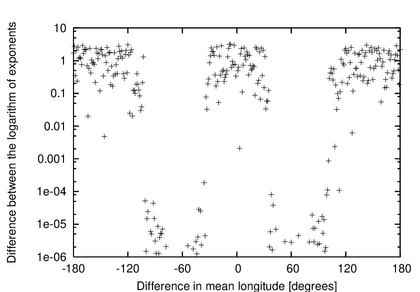
As an initial test, we have compared the LCIs computed by two different integration methods, namely RKN7/8/ and the Lie-integration with the order of $M=8$ . The dynamical system is the spatial Sun – Jupiter – Saturn – test particle spatial restricted four-body system where the latter has the same orbit as the Jupiter has. The LCIs are calculated as the function of the difference in the mean longitudes of Jupiter ( $\lambda_{\mathrm{J}}$ ) and the test particle ( $\lambda_{\mathrm{m}}$ ) while all other 5 initial orbital elements are equal to those of Jupiter. The results are plotted in Fig. 1. In the left panel of Fig. 1, one can see the derived indicators by the method of RKN7/8/, $\mathrm{LCI}_{\mathrm{RKN7/8/}}$ and using Lie-integration, $\mathrm{LCI}_{\mathrm{Lie}}$ as the function of $\Delta\lambda=\lambda_{\mathrm{m}}-\lambda_{\mathrm{J}}$ . In the right panel, the absolute value of the base-10 logarithm of the ratio of the indicators, namely

\chi=\left|\log_{10}\left(\frac{\mathrm{LCI}_{\mathrm{RKN7/8/}}}{\mathrm{LCI}_{\mathrm{Lie}}}\right)\right|,

(77)

are plotted resulted by this two integration method. Note that the integration length is $10^{6}~\mathrm{yrs}$ , therefore the LCIs concerning to regular solutions are saturated around $\approx 10^{-5}-10^{-6}~1/\mathrm{yr}$ . It can easily be seen that in the stable regions (around the two Lagrangian points at $\Delta\lambda=-60^{\circ}$ and $\Delta\lambda=+60^{\circ}$ ) the results of the two methods are very similar, the magnitude of the differences between them is $\approx 10^{-5}$ . In the chaotic regions, the two methods yielded different LCIs but their magnitudes were always the same.

4.1 Performance analysis

We have compared the efficiency of the Lie-integrator and the other implemented integrators. Here we give how much CPU time is required to integrate the equations of motion with RK4, RKN5/6/, RKN7/8/, BS and with the Lie-integration and parallelly the linearized equations to get the result with a previously given accuracy. The ratio of the net CPU times is the relative cost:

\mathrm{cost}^{\mathrm{[other]}}:=\frac{\tau_{\mathrm{CPU}}^{\mathrm{[Lie]}}}{\tau_{\mathrm{CPU}}^{\mathrm{[other]}}}.

(78)

As one can see, the smaller the cost is the more efficient the Lie-integration is. It should be kept in mind that this relative cost does not only depend on the other method but also on the order of the Lie-integration and the desired accuracy. Going into the details, the cost has been measured indirectly by the following way. It can be said that any of the integration algorithms, the RK-based ones, the BS and the Lie-integration use the same CPU time per step independently from the stepsize¹¹ 1 In our tests, in the BS method the adaptive variation of the number of MMID substeps has been disabled, i.e. the extrapolation is performed after the same sequence of number of substeps: it yields an evaluation time which is independent from the stepsize.. Let us denote this atomic CPU time by $\tau_{(0)}^{[\mathrm{method}]}$ . Therefore, if the optimal stepsize $\Delta t_{(\varepsilon)}^{[\mathrm{method}]}$ is known for a given method and accuracy, the total CPU time can easily be calculated:

\tau_{\mathrm{CPU}}^{[\mathrm{method}]}=\tau_{(0)}^{[\mathrm{method}]}\frac{T}{\Delta t_{(\varepsilon)}^{[\mathrm{method}]}},

(79)

where $T$ is the total length of the integration. Because the relative cost is the ratio of two such value of $\tau_{\mathrm{CPU}}$ for two methods, the total length of the integration cancels. The atomic CPU time can easily be measured, the only unknown is the $\Delta t$ optimal stepsize for the different methods. The latter is determined by the following way. The exact mean longitude for the fastest rotating planet is derived for a given time-span (which is defined by the accuracy, see equation (76)) with an appropriately small stepsize. After it, the stepsize is increased iteratively by a bracketing algorithm until the integration yields a mean longitude which differs from the exact one by the $\Delta\lambda$ value determined also by equation (76). We should note that this implies that the stepsize $\Delta t$ is constant during the integration. In Table 1 we summarize these timing values for some values of accuracy and for the Runge-Kutta methods, for the Bulirsch-Stoer method as well as for the Lie-integration method for orders $M=6,\dots,16$ for the dynamical system of Sun -- Jupiter -- Saturn -- test particle extended with the linearized equations of the latter. The second column contains the atomic CPU time²² 2 measured on an Athlon XP 1800+ processor with GCCv4.1.2 compiler, in the units of $10^{-6}$ seconds., while the other three columns show the optimal stepsize $\Delta t_{(\varepsilon)}^{[\mathrm{method}]}$ , derived by the above manner for the accuracies $\varepsilon=2.4\cdot 10^{-11}$ , $2.4\cdot 10^{-12}$ and $2.4\cdot 10^{-13}$ respectively. Thus, the cost can be derived by the fractions of the appropriate values taken from this table, namely:

\mathrm{cost}^{\mathrm{[m1]against[m2]}}=\frac{\tau_{(0)}^{[\mathrm{m1}]}\Delta t_{(\varepsilon)}^{[\mathrm{m2}]}}{\tau_{(0)}^{[\mathrm{m2}]}\Delta t_{(\varepsilon)}^{[\mathrm{m1}]}},

(80)

where $\mathrm{[m1]}$ and $\mathrm{[m2]}$ index the two methods to be compared. We should note that timing values were not only derived for these values of accuracy as it can be read from Table 1 and we have made timing measurements when the linearized equations are omitted. See next sections for more details and for other plots.

4.2 Efficiency as the function of the accuracy

In Fig. 2 the relative cost of the Lie-integration against the RKN7/8/ and the Bulirsch-Stoer integration method are plotted for the three-body problem of Sun – Jupiter – Saturn as the function of the accuracy. Different curves show the cost for different orders of the Lie-integration between $6$ and $16$ . It can easily be seen that for higher orders and below a critical accuracy the Lie-integration is more efficient than RKN7/8/ and for higher orders, the Lie-integration is more efficient than the Bulirsch-Stoer method almost independently from the accuracy. Note that in this plot the linearized equations are omitted from the calculations.

In Fig. 3 we have plotted the cost of the Lie-integration against the methods as above but the dynamical system is extended with a massless test particle and for the latter the linearized equations are also solved. The qualitative behaviour of the cost as the function of the accuracy and the orders of the Lie-series is almost the same as in Fig. 2. We note that the different methods used in the RKN, BS and Lie-integration to evaluate the linearized equations result different number of operations, therefore the costs won’t be exactly the same. Namely, the relative CPU time cost of the Lie-integration against the other methods is slightly larger when the linearized equations are solved parallely.

As a conclusion, we can say that omitting the linearized part orders below $M\approx 10$ the Lie-integration method is inferior to the RKN7/8/, while the equations are extended with the linearized equations for the massless particle, the Lie-integration is more effective than RKN7/8/ for orders larger than $M\approx 12$ below a certain accuracy about $\varepsilon\approx 10^{-11}$ . Comparing with the BS method, the Lie-integration is more effective for orders larger than $M\approx 8$ and $M\approx 10$ when the linearized equations are omitted or not, almost independently from the accuracy. We note that the Lie-integration is effective with more than a magnitude (or more) than the lower-order Runge-Kutta methods, as it can easily be derived from Table. 1 and equation (80).

4.3 Efficiency as the function of the order

As it was written in the introduction, the method of Lie-integration approximates the Taylor-expansion of the solution up to a finite order. One can easily prove that the appropriate order, $n$ of a Taylor-series to obtain a certain accuracy of a periodic function defined on an interval is proportional to the length, $L$ of this interval. The concept of the proof is as follows. An adequately smooth periodic function can be approximated as a sum of sine (and cosine) functions, the so-called Fourier terms. The sine function, $\sin(x)$ can be expanded as

\sin(x)=\sum\limits_{k=0}^{\infty}(-1)^{k}\frac{x^{2k+1}}{(2k+1)!}.

(81)

To obtain an accuracy of unity, the last ( $n=2k+1$ th) term of the series should be the solution of $x^{n}\equiv L^{n}\approx n!$ . Therefore, using Stirling’s approximation, one gets

n\log L=\log(n!)\approx n\log n-n,

(82)

so $n\approx\mathrm{e}\cdot L$ , which means $n\sim L$ . This is true for all Fourier terms of the expansion of a periodic function.

Thus one can assume that to obtain a certain accuracy, the $M$ number of the terms in the Lie-series is proportional to the length of the integration stepsize, namely $\Delta t\approx\kappa M$ . The total number of arithmetical operations, therefore the required CPU time is a quadratic function of the order $M$ : $\tau_{\mathrm{CPU}}=\mathrm{Ordo}(M^{2})$ . To be more precise, the required CPU time is $\tau_{\mathrm{CPU}}=\alpha+\beta M+\gamma M^{2}$ , for smaller $M$ ’s, the first two terms, $\alpha$ and $\beta M$ are not negligible. Therefore, to integrate the equations over an interval $T$ requires

\tau_{\mathrm{CPU}}^{\mathrm{total}}\approx(\alpha+\beta M+\gamma M^{2})\frac{T}{\Delta t}=(\alpha+\beta M+\gamma M^{2})\frac{T}{\kappa M}

(83)

CPU time, which, depending on the ratios of the constants $\alpha$ , $\beta$ and $\gamma$ has a minimum corresponding to the optimal order of the Lie-integration method.

We have tested this type of dependency of the CPU time on the order of the Lie-integration. The results are plotted in Fig. 4, for three values of accuracy, while the dynamical system is the restricted four body problem of Sun – Jupiter – Saturn – test particle extended with the linearized equations respecting to the latter. As it was assumed above, the relative cost has a minimum corresponding to the optimal order and the value of this minimum is around $M\approx 13-15$ , depending on the accuracy. It can also be seen that for larger values of $M$ the cost increases which means worse efficiency, as it is expected from equation (83). What is more interesting that the position of the minimum clearly depends on the accuracy: the better the accuracy is the larger the optimal value of $M$ is. This might imply another kind of adaptive integration method where not only the stepsize varies but the order of the Lie-integration.

4.4 Implemetaion of the method

We have implemented the method of Lie-integration of the $N$ -body problem as a standalone ANSI C program, extended with the linearized equations and the capability to calculate the LCIs. The version of the program which can integrate the motion of 1+3 bodies and was used in our benchmarks can be downloaded from the address http://cm.elte.hu/lie as a single .tar.gz archive. The full version which is capable to integrate the motion of arbitrary number of bodies can be requested from the first author via e-mail. All versions of this code are designed to work on UNIX-like environments.

5 Discussion and summary

In this paper we have presented a lemma with which recurrence relations can be derived for the Lie-integration of linearized equations. We have demonstrated the usage of this lemma on the Hénon-Heiles system, and thereafter applied it to the equations of the $N$ -body problem, including the non-inertial equations where the origin of the reference frame is fixed to one of the bodies. Our performance comparisons have shown that although these recurrence formulae are rather complicated, they can efficiently be used for integrations where high accuracy is required. We have investigated realistic dynamical systems for these comparisons: using the lemma, the recurrence relations were determined and using the Lie-integration technique, the LCIs for a fictitious asteroid was computed. The method of LCIs is the basis for many modern chaos detection methods, therefore our lemma and the derived Lie-integration method can widely be used in various kind of dynamical investigations, providing a faster alternative to the currently used techniques. We have checked the efficiency as the function of the order and accuracy. These tests have shown that the Lie-integration is definitely more effective than the classical RK4 and RKN5/6/ integration method and above a certain accuracy about $\varepsilon\approx 10^{-11}$ , the Lie-integration is more effective than the method of RKN7/8/ for orders larger than $M=10$ or $M=8$ , whether the linearized equations are evaluated parallelly or not. We found that the Lie-integration is more effective than the BS integrator for orders larger than $M\approx 10$ , almost independently from the accuracy.

Further studies are already ongoing concerning this problem. First, there could be several possibilities for optimization in the actual implementation of the Lie-integration: we expect that the re-ordering of the highly nested loops and/or the introduction of new auxiliary variables yield better performance. Second, some aspects of the Lie-integration should better be analysed and understood, including the long-term error propagation in higher orders which is the basis of the adaptive extensions of this integration method. And last, we are going to develop a more general code which is not only capable of the calculation of LCIs but can be extended with other chaos indicators.

References

Chambers (1999) Chambers, J. E., 1999, MNRAS, 304, 793
Cincotta & Simó (2000) Cincotta, P. M., Simó, C., 2000, ApJS, 147, 205
Dormand & Prince (1978) Dormand, J. R., Prince, P. J, 1978, CeMDA, 18, 223
Fehlberg (1972) Fehlberg, E., 1972, NASA Technical Report, R381
Froeschlé et al. (1997) Froeschlé, C., Lega, E., Gonczi, R., 1997, CeMDA, 67, 41
Godźiewski et al. (2001) Godźiewski, K., Bois, E., Maciejewski, A. J., Kiseleva-Eggleton, L., 2001, A&A, 378, 569
Gröbner & Knapp (1967) Gröbner, W., Knapp, H., 1967, ”Contributions to the Method of Lie-Series”
Hénon & Heiles (1964) Hénon, M., Heiles, C., 1964, AJ, 69, 73
Hanslmeier & Dvorak (1984) Hanslmeier, A., Dvorak, R., 1984, A&A, 132, 203
Laskar (1990) Laskar, J., 1990, Icarus, 88, 266
Lyapunov (1907) Lyapunov, A. M., 1907, Ann. Math. Studies 17, Princeton (1947)
Milani & Nobili (1988) Milani, A., Nobili, A., 1988, CeMDA, 43, 1
Oseledec (1968) Oseledec, V. I., 1968, Trans. Moscow Math. Soc., 19, 197
Poincaré (1899) Poincaré, H., 1899, Méthodes nouvelles de la mécanique céleste, Tome 3 (Gauthier Villars, Paris 1899)
Press et al. (1992) Press, W. H., Teukolsky, S. A., Vetterling, W.T., Flannery, B.P., 1992, Numerical Recipes in C: the art of scientific computing, Second Edition, Cambridge University Press

Appendix A Recurrence relations for the $N$ -body problem

Using the notations defined in Section 3.1, we derive the recurrence relations for the equations of motion for the $N$ -body problem.

As we have shown in Section 3.1 the Lie-operator of the equations of motion is

L_{0}=v_{im}D_{im}-G\sum\limits_{i}\left[\left(\sum\limits_{j=1,j\neq i}^{K}m_{j}\phi_{ij}A_{ijm}\right)\Delta_{im}\right].

(84)

This implies that the first Lie-derivatives of the coordinates and velocities are the right-hand side of the equations of motion, namely

	$\displaystyle L_{0}x_{im}$	$\displaystyle=$	$\displaystyle v_{im},$		(85)
	$\displaystyle L_{0}v_{im}$	$\displaystyle=$	$\displaystyle-G\sum\limits_{j=1,j\neq i}^{K}m_{j}\rho_{ij}^{-3}(x_{jm}-x_{im})=-G\sum\limits_{j=1,j\neq i}^{K}m_{j}\phi_{ij}A_{ijm}.$

The distance $\rho_{ij}$ does not depend on the velocities, like so $\phi_{ij}$ , therefore their Lie-derivatives can easily be calculated:

L_{0}\rho_{ij}=\sum\limits_{k}v_{km}D_{km}\rho_{ij}.

(86)

Therefore,

$\displaystyle L_{0}\rho_{ij}$	$\displaystyle=$	$\displaystyle\sum\limits_{k}v_{km}\frac{\partial}{\partial x_{km}}\sqrt{\sum\limits_{m}(x_{jm}-x_{im})(x_{jm}-x_{im})}=\sum\limits_{k}v_{km}\frac{\frac{\partial}{\partial x_{km}}\left(\sum\limits_{m}(x_{jm}-x_{im})(x_{jm}-x_{im})\right)}{2\sqrt{\sum\limits_{m}(x_{jm}-x_{im})(x_{jm}-x_{im})}}=$	(87)
	$\displaystyle=$	$\displaystyle\sum\limits_{k}v_{km}\left[\frac{1}{2\rho_{ij}}\left(2(x_{jm}-x_{im})(\delta_{kj}-\delta_{ki})\right)\right]=\sum\limits_{k}v_{km}\rho_{ij}^{-1}\left[(x_{jm}-x_{im})(\delta_{kj}-\delta_{ki})\right]=$
	$\displaystyle=$	$\displaystyle\rho_{ij}^{-1}\left[(v_{jm}-v_{im})(x_{jm}-x_{im})\right]=\rho_{ij}^{-1}B_{jim}A_{jim}=\rho_{ij}^{-1}\Lambda_{ji}=\rho_{ij}^{-1}\Lambda_{ij}.$

Now one can calculate the Lie-derivative of $\phi_{ij}=\rho_{ij}^{-3}$ :

L_{0}\phi_{ij}=L_{0}(\rho_{ij}^{-3})=-3\rho_{ij}^{-4}L_{0}\rho_{ij}=-3\rho_{ij}^{-5}\Lambda_{ij}=\rho_{ij}^{-2}(-3\phi_{ij}\Lambda_{ij}).

(88)

With mathematical induction, one can prove that

L_{0}^{n+1}\phi_{ij}=\rho_{ij}^{-2}\sum\limits_{k=0}^{n}\left[-3{n\choose k}-2{n\choose k+1}\right]L_{0}^{n-k}\phi_{ij}L_{0}^{k}\Lambda_{ij}.

(89)

For $n=0$ this equation is equivalent to equation (88). Let us assume that this is true for all $m\leq n$ , and calculate $L_{0}^{n+2}\phi_{ij}$ :

$\displaystyle L_{0}^{n+2}\phi_{ij}$	$\displaystyle=$	$\displaystyle L_{0}\left(\rho_{ij}^{-2}\sum\limits_{k=0}^{n}\left[-3{n\choose k}-2{n\choose k+1}\right]L_{0}^{n-k}\phi_{ij}L_{0}^{k}\Lambda_{ij}\right)=$	(90)
	$\displaystyle=$	$\displaystyle\underbrace{L_{0}\left(\rho_{ij}^{-2}\right)\cdot\left(\rho_{ij}^{2}L_{0}^{n+1}\phi_{ij}\right)}_{\mathrm{Term~1}}+\underbrace{\rho_{ij}^{-2}\sum\limits_{k=0}^{n}\left[-3{n\choose k}-2{n\choose k+1}\right]L_{0}^{n+1-k}\phi_{ij}L_{0}^{k}\Lambda_{ij}}_{\mathrm{Term~2}}+$
		$\displaystyle+\underbrace{\rho_{ij}^{-2}\sum\limits_{k=0}^{n}\left[-3{n\choose k}-2{n\choose k+1}\right]L_{0}^{n-k}\phi_{ij}L_{0}^{k+1}\Lambda_{ij}}_{\mathrm{Term~3}}=\%.$

The first term is

L_{0}\left(\rho_{ij}^{-2}\right)\cdot\left(\rho_{ij}^{2}L_{0}^{n+1}\phi_{ij}\right)=-2\rho_{ij}^{-1}\Lambda_{ij}\phi_{ij}\rho_{ij}^{2}L_{0}^{n+1}\phi_{ij}=\rho_{ij}^{-2}\left(-2L_{0}^{n+1}\phi_{ij}\Lambda_{ij}\right).

(91)

We can increase the upper limit of the first summation of term 2 in equation (90) from $n$ to $n+1$ , since in the appearing new terms, the factors ${n\choose n+1}$ and ${n\choose n+2}$ are zero by definition. To unify term 1 and term 3, we introduce a new index, $k^{\prime}=k+1$ in term 3 of equation (90):

\rho_{ij}^{-2}\sum\limits_{k=0}^{n}\left[-3{n\choose k}-2{n\choose k+1}\right]L_{0}^{n-k}\phi_{ij}L_{0}^{k+1}\Lambda_{ij}=\rho_{ij}^{-2}\sum\limits_{k^{\prime}=1}^{n+1}\left[-3{n\choose k^{\prime}-1}-2{n\choose k^{\prime}}\right]L_{0}^{n+1-k^{\prime}}\phi_{ij}L_{0}^{k^{\prime}}\Lambda_{ij}.

(92)

Note that if we substitute $k^{\prime}=0$ into the expression after the summation, we get the same what equation (91) is, therefore the latter can be inserted into the summation of equation (92) while the lower limit of $k^{\prime}=1$ is replaced to $k^{\prime}=0$ . Therefore:

\%=\rho_{ij}^{-2}\sum\limits_{k^{\prime}=0}^{n+1}\left[-3{n\choose k^{\prime}}-2{n\choose k^{\prime}+1}-3{n\choose k^{\prime}-1}-2{n\choose k^{\prime}}\right]L_{0}^{n+1-k^{\prime}}\phi_{ij}L_{0}^{k^{\prime}}\Lambda_{ij}=\%.

(93)

Using the relation ${n\choose k}+{n\choose k+1}={n+1\choose k+1}$ , we get

-3{n\choose k}-2{n\choose k+1}-3{n\choose k-1}-2{n\choose k}=-3{n+1\choose k}-2{n+1\choose k+1},

(94)

therefore we could simplify equation (93):

\%=\rho_{ij}^{-2}\sum\limits_{k=0}^{n+1}\left[-3{n+1\choose k}-2{n+1\choose k+1}\right]L_{0}^{n+1-k}\phi_{ij}L_{0}^{k}\Lambda_{ij}.

(95)

Comparing equation (95) with equation (89), we conclude that the relation is proven. For simplicity, we define

F_{nk}:=-3{n\choose k}-2{n\choose k+1}.

(96)

Continuing the derivation of the recurrence formulae, we calculate the higher order Lie-derivatives of $\Lambda_{ij}$ using the binomial theorem:

L_{0}^{n}\Lambda_{ij}=\sum\limits_{k=0}^{n}{n\choose k}L_{0}^{k}A_{ijm}L_{0}^{n-k}B_{ijm}=\sum\limits_{k=0}^{n}{n\choose k}(L_{0}^{k}x_{im}-L_{0}^{k}x_{jm})(L_{0}^{n-k}v_{im}-L_{0}^{n-k}v_{jm}).

(97)

In the equations of motion the term $\phi_{ij}A_{ijm}$ appears, its higher order Lie-derivatives can also be calculated like the last relation for $L_{0}^{n}\Lambda_{ij}$ :

L_{0}^{n}(\phi_{ij}A_{ijm})=\sum\limits_{k=0}^{n}{n\choose k}L_{0}^{k}\phi_{ij}(L_{0}^{n-k}x_{im}-L_{0}^{n-k}x_{jm}).

(98)

To summarize our results the complete set of the recurrence relations for the equations of motion can be found in equations (49)-(54).

Appendix B Derivation of the linearized equations

To obtain the recurrence relations for the linearized equations, we apply the operator $\Xi\cdot\mathcal{D}$ to equations (49)-(54). We note that the operator $\Xi\cdot\mathcal{D}$ is linear,

\Xi\cdot\mathcal{D}(pa+qb)=p(\Xi\cdot\mathcal{D}a)+q(\Xi\cdot\mathcal{D}b),

(99)

where $a$ and $b$ are continuous functions while $p$ and $q$ are constants, and one can use Leibniz’s rule:

\Xi\cdot\mathcal{D}(ab)=(\Xi\cdot\mathcal{D}a)b+a(\Xi\cdot\mathcal{D}b).

(100)

Moreover, we should note that the operators $\Xi\cdot\mathcal{D}$ and $L$ cannot be commuted, $\Xi\cdot\mathcal{D}L\neq L\Xi\cdot\mathcal{D}$ .

For the first three equations, we get

$\displaystyle L^{n+1}\xi_{im}$	$\displaystyle=$	$\displaystyle\Xi\cdot\mathcal{D}L^{n+1}x_{im}=\Xi\cdot\mathcal{D}L^{n}v_{im}=L^{n}\eta_{im},$	(101)
$\displaystyle L^{n}\alpha_{ijm}$	$\displaystyle=$	$\displaystyle L^{n}\xi_{im}-L^{n}\xi_{jm},$	(102)
$\displaystyle L^{n}\beta_{ijm}$	$\displaystyle=$	$\displaystyle L^{n}\eta_{im}-L^{n}\eta_{jm}.$	(103)

For $\Xi\cdot\mathcal{D}\Lambda_{ij}$ we can use the linear property and apply Leibniz’s rule:

	$\displaystyle\Xi\cdot\mathcal{D}L^{n}\Lambda_{ij}$	$\displaystyle=$	$\displaystyle\sum\limits_{k=0}^{n}{n\choose k}\left[(\Xi\cdot\mathcal{D}L^{k}A_{ijm})L^{n-k}B_{ijm}+L^{k}A_{ijm}(\Xi\cdot\mathcal{D}L^{n-k}B_{ijm})\right]=$		(104)
		$\displaystyle=$	$\displaystyle\sum\limits_{k=0}^{n}{n\choose k}\left[L^{k}\alpha_{ijm}L^{n-k}B_{ijm}+L^{k}A_{ijm}L^{n-k}\beta_{ijm})\right].$		(104)

Here we applied the identities $\Xi\cdot\mathcal{D}L^{n}A_{ijm}=L^{n}\alpha_{ijm}$ and $\Xi\cdot\mathcal{D}L^{n}B_{ijm}=L^{n}\beta_{ijm}$ . For the calculation of $\Xi\cdot\mathcal{D}L^{n+1}\phi_{ij}$ we follow the same procedure:

	$\displaystyle\Xi\cdot\mathcal{D}L^{n+1}\phi_{ij}$	$\displaystyle=$	$\displaystyle(\Xi\cdot\mathcal{D})\left[\rho_{ij}^{-2}\sum_{k=0}^{n}F_{nk}L^{n-k}\phi_{ij}L^{k}\Lambda_{ij}\right]=$		(105)
		$\displaystyle=$	$\displaystyle(\Xi\cdot\mathcal{D}\rho_{ij}^{-2})(\rho_{ij}^{2}L^{n+1}\phi_{ij})+\rho_{ij}^{-2}\sum\limits_{k=0}^{n}F_{nk}\left[(\Xi\cdot\mathcal{D}L^{n-k}\phi_{ij})L^{k}\Lambda_{ij}+L^{n-k}\phi_{ij}(\Xi\cdot\mathcal{D}L^{k}\Lambda_{ij})\right].$		(105)

The only unknown factor in equation (105) is the quantity $\Xi\cdot\mathcal{D}\rho_{ij}^{-2}$ . We can calculate it easily, because $\rho_{ij}^{-2}$ only depends by definition on the coordinates:

\Xi\cdot\mathcal{D}\rho_{ij}^{-2}=\xi_{km}D_{km}(\rho_{ij}^{-2})=\xi_{km}(-2)\rho_{ij}^{-3}D_{km}\rho_{ij}=\left(-2\rho_{ij}^{-3}\right)\xi_{km}D_{km}\rho_{ij}=\%.

(106)

The expression $\xi_{km}D_{km}\rho_{ij}$ can be calculated like equation (86), where we replace $v_{km}$ by $\xi_{km}$ :

\xi_{km}D_{km}\rho_{ij}=\rho_{ij}^{-1}(\xi_{im}-\xi_{jm})(x_{im}-x_{jm})=\rho_{ij}^{-1}\alpha_{ijm}A_{ijm}.

(107)

Thus, we get

\%=-2\rho_{ij}^{-4}\alpha_{ijm}A_{ijm}.

(108)

Adding all terms together, we obtain

\Xi\cdot\mathcal{D}L^{n+1}\phi_{ij}=-2\rho_{ij}^{-2}\alpha_{ijm}A_{ijm}L^{n+1}\phi_{ij}+\rho_{ij}^{-2}\sum\limits_{k=0}^{n}F_{nk}\left[(\Xi\cdot\mathcal{D}L^{n-k}\phi_{ij})L^{k}\Lambda_{ij}+L^{n-k}\phi_{ij}(\Xi\cdot\mathcal{D}L^{k}\Lambda_{ij})\right].

(109)

The derivation of $L^{n+1}\eta_{im}=\Xi\cdot\mathcal{D}L^{n+1}v_{im}$ is the following:

$\displaystyle L^{n+1}\eta_{im}$	$\displaystyle=$	$\displaystyle\Xi\cdot\mathcal{D}L^{n+1}v_{im}=-G\sum\limits_{j=1,j\neq i}^{K}m_{j}\left\{\sum\limits_{k=0}^{n}{n\choose k}\Xi\cdot\mathcal{D}\left(L^{k}\phi_{ij}L^{n-k}A_{ijm}\right)\right\}=$	(110)
	$\displaystyle=$	$\displaystyle-G\sum\limits_{j=1,j\neq i}^{K}m_{j}\left\{\sum\limits_{k=0}^{n}{n\choose k}\left[(\Xi\cdot\mathcal{D}L^{k}\phi_{ij})L^{n-k}A_{ijm}+L^{k}\phi_{ij}(\Xi\cdot\mathcal{D}L^{n-k}A_{ijm})\right]\right\}=$
	$\displaystyle=$	$\displaystyle-G\sum\limits_{j=1,j\neq i}^{K}m_{j}\left\{\sum\limits_{k=0}^{n}{n\choose k}\left[(\Xi\cdot\mathcal{D}L^{k}\phi_{ij})L^{n-k}A_{ijm}+L^{k}\phi_{ij}L^{n-k}\alpha_{ijm}\right]\right\}.$

Now we obtained the recurrence relations for all of the linearized coordinates, velocities and the auxiliary variables $\Xi\cdot\mathcal{D}\Lambda_{ij}$ , $\Xi\cdot\mathcal{D}\phi_{ij}$ . The complete set of these equations are summarized in equations (61)-(66).

Appendix C Motion in a reference frame fixed to one of the bodies

Throughout the derivation of the recurrence relations, we can use the fact that the partial differential operators $\frac{\partial}{\partial r_{im}}$ and $\frac{\partial}{\partial w_{im}}$ are equivalent to $D_{im}=\frac{\partial}{\partial x_{im}}$ and $\Delta_{im}=\frac{\partial}{\partial v_{im}}$ , because the variables differ only in a constant ( $x_{0m}$ and $v_{0m}$ , respectively). We have to define the new variable $\Lambda_{i}=r_{im}w_{im}$ . The derivation of the recurrence relations can be done following the steps of Appendix A and Appendix B: the quantities $\rho_{i}$ , $\phi_{i}$ and $\Lambda_{i}$ have the same properties for the Lie-derivation as $\rho_{ij}$ , $\phi_{ij}$ and $\Lambda_{ij}$ , respectively, therefore all of the induction steps can be done in the appropriate way.

Thus, the recurrence relations for the $N$ -body problem around a fixed centre can be written as

$\displaystyle L^{n+1}r_{im}$	$\displaystyle=$	$\displaystyle L^{n}w_{im},$	(111)
$\displaystyle L^{n}A_{ijm}$	$\displaystyle=$	$\displaystyle L^{n}r_{im}-L^{n}r_{jm},$	(112)
$\displaystyle L^{n}B_{ijm}$	$\displaystyle=$	$\displaystyle L^{n}w_{im}-L^{n}w_{jm},$	(113)
$\displaystyle L^{n}\Lambda_{i}$	$\displaystyle=$	$\displaystyle\sum\limits_{k=0}^{n}{n\choose k}L^{k}r_{im}L^{n-k}w_{im},$	(114)
$\displaystyle L^{n}\Lambda_{ij}$	$\displaystyle=$	$\displaystyle\sum\limits_{k=0}^{n}{n\choose k}L^{k}A_{ijm}L^{n-k}B_{ijm},$	(115)
$\displaystyle L^{n+1}w_{im}$	$\displaystyle=$	$\displaystyle-G(\mathcal{M}+m_{i})\sum\limits_{k=0}^{n}{n\choose k}L^{k}\phi_{i}L^{n-k}r_{im}-G\sum\limits_{j=1,j\neq i}^{K}m_{j}\sum\limits_{k=0}^{n}{n\choose k}\left[L^{k}\phi_{ij}L^{n-k}A_{ijm}+L^{k}\phi_{j}L^{n-k}r_{jm}\right],$	(116)
$\displaystyle L^{n+1}\phi_{i}$	$\displaystyle=$	$\displaystyle\rho_{i}^{-2}\sum\limits_{k=0}^{n}F_{nk}L^{n-k}\phi_{i}L^{k}\Lambda_{i},$	(117)
$\displaystyle L^{n+1}\phi_{ij}$	$\displaystyle=$	$\displaystyle\rho_{ij}^{-2}\sum\limits_{k=0}^{n}F_{nk}L^{n-k}\phi_{ij}L^{k}\Lambda_{ij}.$	(118)

Let us denote the linearized of $r_{im}$ and $w_{im}$ by $\xi_{im}$ and $\eta_{im}$ , respectively. Since $\alpha_{ijm}=\xi_{im}-\xi_{jm}$ and $\beta_{ijm}=\eta_{im}-\eta_{jm}$ , for the linearized equations the calculations yield

$\displaystyle L^{n+1}\xi_{im}$	$\displaystyle=$	$\displaystyle L^{n}\eta_{im},$	(119)
$\displaystyle L^{n}\alpha_{ijm}$	$\displaystyle=$	$\displaystyle L^{n}\xi_{im}-L^{n}\xi_{jm},$	(120)
$\displaystyle L^{n}\beta_{ijm}$	$\displaystyle=$	$\displaystyle L^{n}\eta_{im}-L^{n}\eta_{jm},$	(121)
$\displaystyle\Xi\cdot\mathcal{D}L^{n}\Lambda_{i}$	$\displaystyle=$	$\displaystyle\sum\limits_{k=0}^{n}{n\choose k}\left(L^{k}\xi_{im}L^{n-k}w_{im}+L^{k}r_{im}L^{n-k}\eta_{im}\right),$	(122)
$\displaystyle\Xi\cdot\mathcal{D}L^{n}\Lambda_{ij}$	$\displaystyle=$	$\displaystyle\sum\limits_{k=0}^{n}{n\choose k}\left(L^{k}\alpha_{ijm}L^{n-k}B_{ijm}+L^{k}A_{ijm}L^{n-k}\beta_{ijm}\right),$	(123)
$\displaystyle L^{n+1}\eta_{im}$	$\displaystyle=$	$\displaystyle-G(\mathcal{M}+m_{i})\sum\limits_{k=0}^{n}{n\choose k}\left[(\Xi\cdot\mathcal{D}L^{k}\phi_{i})L^{n-k}r_{im}+L^{k}\phi_{i}L^{n-k}\xi_{im}\right]-$	(124)
		$\displaystyle-G\sum\limits_{j=1,j\neq i}^{K}m_{j}\sum\limits_{k=0}^{n}{n\choose k}\left[(\Xi\cdot\mathcal{D}L^{k}\phi_{ij})L^{n-k}A_{ijm}+L^{k}\phi_{ij}L^{n-k}\alpha_{ijm}+(\Xi\cdot\mathcal{D}L^{k}\phi_{j})L^{n-k}r_{jm}+L^{k}\phi_{j}L^{n-k}\xi_{jm}\right],$	(124)
$\displaystyle\Xi\cdot\mathcal{D}L^{n+1}\phi_{i}$	$\displaystyle=$	$\displaystyle-2\rho_{i}^{-2}\xi_{im}r_{im}L^{n+1}\phi_{i}+\rho_{i}^{-2}\sum\limits_{k=0}^{n}F_{nk}\left[(\Xi\cdot\mathcal{D}L^{n-k}\phi_{i})L^{k}\Lambda_{i}+L^{n-k}\phi_{i}(\Xi\cdot\mathcal{D}L^{k}\Lambda_{i})\right],$	(125)
$\displaystyle\Xi\cdot\mathcal{D}L^{n+1}\phi_{ij}$	$\displaystyle=$	$\displaystyle-2\rho_{ij}^{-2}\alpha_{ijm}A_{ijm}L^{n+1}\phi_{ij}+\rho_{ij}^{-2}\sum\limits_{k=0}^{n}F_{nk}\left[(\Xi\cdot\mathcal{D}L^{n-k}\phi_{ij})L^{k}\Lambda_{ij}+L^{n-k}\phi_{ij}(\Xi\cdot\mathcal{D}L^{k}\Lambda_{ij})\right].$	(126)

Appendix D Speed-up considerations

Introducing new variables, the required number of arithmetical operations can be decreased in equations (111)-(118) and equations (119)-(126). Namely, the calculation of $L^{n+1}w_{im}$ and $L^{n+1}\eta_{im}$ can be written as

	$\displaystyle L^{n+1}w_{im}$	$\displaystyle=$	$\displaystyle-G(\mathcal{M}+m_{i})S^{[n]}_{im}-G\sum\limits_{j=1,j\neq i}^{K}m_{j}\left(S^{[n]}_{ijm}+S^{[n]}_{jm}\right),$		(127)
	$\displaystyle L^{n+1}\eta_{im}$	$\displaystyle=$	$\displaystyle-G(\mathcal{M}+m_{i})\Sigma^{[n]}_{im}-G\sum\limits_{j=1,j\neq i}^{K}m_{j}\left(\Sigma^{[n]}_{ijm}+\Sigma^{[n]}_{jm}\right),$		(128)

where the new variables are

$\displaystyle S^{[n]}_{im}$	$\displaystyle=$	$\displaystyle\sum\limits_{k=0}^{n}{n\choose k}L^{k}\phi_{i}L^{n-k}r_{im},$	(129)
$\displaystyle S^{[n]}_{ijm}$	$\displaystyle=$	$\displaystyle\sum\limits_{k=0}^{n}{n\choose k}L^{k}\phi_{ij}L^{n-k}A_{ijm},$	(130)
$\displaystyle\Sigma^{[n]}_{im}$	$\displaystyle=$	$\displaystyle\sum\limits_{k=0}^{n}{n\choose k}\left[(\Xi\cdot\mathcal{D}L^{k}\phi_{i})L^{n-k}r_{im}+L^{k}\phi_{i}L^{n-k}\xi_{im}\right],$	(131)
$\displaystyle\Sigma^{[n]}_{ijm}$	$\displaystyle=$	$\displaystyle\sum\limits_{k=0}^{n}{n\choose k}\left[(\Xi\cdot\mathcal{D}L^{k}\phi_{ij})L^{n-k}A_{ijm}+L^{k}\phi_{ij}L^{n-k}\alpha_{ijm}\right].$	(132)

The implementation of the above relations can increase the speed of the calculations by 20%-30%, depending on the number of the bodies.

Solving Linearized Equations of the NN-body Problem Using the Lie-integration MethodSolving Linearized Equations of the NN-body Problem Using the Lie-integration Method–D2007