Discontinuity in the specific heat of a weakly interacting Bose gas

⁴He becomes superfluid below 2.18K, so called $\lambda$ point, at low atmospheric pressure. The specific heat of liquid ⁴He is infinitesimal around 0$K$, and rises with $T^{2/3}$ until it reaches a the $\lambda$ point that shows a dramatic divergence, and then decreases tending asymptotically to a constant classical value. The transition is known as the strongest degeneracy effect of a boson system, but it is still not fully understood. Many physicists have tried to reproduce the discontinuity of the specific since the discovery of the transition, but even until now very little researches has done it successfully.

Kikuchi et al. applied a partition function proposed by Feynman to an Ising model-like 2D cubic lattice and considering nearest-neighbors only, they calculated the specific heat at $T_{c}$ numerically kikuchi. Although they produced the discontinuity of the specific heat, their method strongly depends on various atomic bond models and experimental variables. Therefore, this semi-empirical and numerical method could not give any formula between the $\lambda$ transition and the interaction strength.

The objective of this paper is to reproduce the discontinuity of the specific heat of a homogeneous, dilute, and weakly interacting (HDWI) Bose system analytically. Through the application of a simple statistical method. the relation between the $\lambda$ transition and the interacting strength will be obtained. The weakly interacting Bose model may prove useful to understand the strongly interacting liquid ⁴He. We will write this argument in D-dimensions ($2<D\leq 3$) for better applicability.

The dilute is expressed by a dimensionless gas parameter $\gamma=n(1)a$, where $n(1)$ is the one-dimensional number density and $a$ is the $s$-wave scattering length. In a homogeneous system, the density in D-dimensions is expressed as $n(D)=n(1)^{D}$. In a repulsive dilute gas, $\gamma$ is positive and much less than 1. The $\gamma$ of liquid ⁴He is known as on the order of one-half, and therefore the HDWI model is different from the real Bose system.

For a momentum-independent interaction $g(D)$, the mean field contribution to the self-energy is $n(D)g(D)$. Then, the dispersion relation of the weakly interacting Bose gas can be written as

where $\varepsilon_{0}=p^{2}/2m$. The $g(D)$ is the positive coupling constant in D-dimensions, where $2<D\leq 3$. With the hard-sphere interaction, it is well-known in 3D as $g(3)=4\pi\hbar^{2}a/m.$ The dispersion relation corresponds to a short-wavelength range in the Bogoliubov energy spectrum bogol. The exact form of the interaction is $2n(D)g(D)$ instead of $n(D)g(D)$ because the two mean field contributions to the self-energy from Hartree and Fock are equal. However, we will use Eq. (1) because the factor of 2 is not a key concept here.

The grand partition function of the momentum-independent potential is given from Eq. (1) as

where $\beta=1/k_{B}T$. The $z$ is the fugacity given by $z=e^{\beta\mu}$ and 1 below $T_{c}$. The $\mu$ is the chemical potential, which is $0$ below the $T_{c}$ and negative above the $T_{c}$. The $z_{e}$ is the effective fugacity given by

Note that $0\leq z_{e}<1$. As $T\rightarrow T_{c}$, then $z_{e}\rightarrow e^{-\beta_{c}ng}\equiv\eta_{c}$. Note that $0<\eta_{c}<1$, and 1 for the non-interacting Bose system. The effective chemical potential is written in the same way : $\mu_{e}=\mu-ng$. It is $-ng$ instead of zero below $T_{c}$. Even for a momentum-independent potential, it shifts the transition temperature.

The equation of the state of the interacting system in D-dimensions is written from Eq. (2) as huang

where $\lambda=\sqrt{2\pi\hbar^{2}/mk_{B}T}$ is the thermal wavelength, and $g_{s}(z)=\sum_{l=1}^{\infty}z^{l}/l^{s}$ is the Bose function. The only difference of the formula from the non-interacting model is the effective fugacity $z_{e}$, and the information of the coupling constant $g(D)$ is in it.

Let $T_{o}\equiv 2\pi\hbar^{2}n(2)/mk_{B}=1$ since $n(D)^{\frac{2}{D}}=n(2)$. It is about 5.92K for liquid ⁴He. In this way from Eq. (4) the relation of the transition temperature between ideal and interacting system is written as

The right-hand side is actually $T_{o}$. In this way the $T_{c}(3)$ of the interacting systems is obtained self-consistently by numerical method as

The relation between $T_{c}(3)$ and $T_{c}^{0}(3)$ is also written as the power series of the $\gamma$. The leading order in 3D is

We may use the value obtained from the numerical simulation as $c\simeq 1.3$ arnold; kashunikov.

We obtain the internal energy in D-dimensions from $U(T)=-(\partial/\partial\beta)_{v}\ln{\cal Q}(z,n,T)$.
At $T<T_{c}$ :

and at $T>T_{c}$ :

The internal energy is continous at $T_{c}$ as $\lim_{T\rightarrow T_{c}}\Delta U(T)=0$

The specific heat at constant volume is obtained as $C_{v}=(\partial/\partial T)_{v}U(T)$. Therefore, we have $C_{v}$ below and above the transition temperature in 3D.
At $T<T_{c}$ :

and at $T>T_{c}$ :

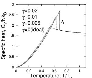
We used Eq. (5) and the relation $\beta n(3)g(3)=2\gamma/T$ and $\partial\eta/\partial T=2\gamma\eta/T^{2}$. The discontinuity of the $C_{v}$ at $T_{c}$ is

The non-interacting limit goes to the well-known results as $\lim_{\gamma\rightarrow 0}\Delta C_{v}=0$, since $g_{\frac{1}{2}}(1)$ goes to infinity.

The effective fugacity $z_{e}(T)=ze^{-\eta}$ is shown in Fig. 1. It downshifts from 1 as the interaction is increasing. The $C_{v}$ at $D=3$ is shown in Fig. 2, too.

We considered the short-wavelength range only in the dispersion relation, and applied a simple mean field based statistical mechanics to the homogeneous, dilute, and weakly interacting Bose system. In spite of the simplicity of the system, it successfully produced the relation between the discontinuity of the specific heat and the interaction strength of the model clearly.

References

- (1) R. Kikuchi, H.H. Denman, and C.L. Schreiber, Phys. Rev. 119, 1823 (1960).
- (2) N.N. Bogoliubov, J. Phys. (USSR) 11, 23 (1947).
- (3) P. Arnold and G. Moore, Phys. Rev. Lett. 87, 120401 (2001).
- (4) V.A. Kashurnikov, N.V. Prokof’ev, and B. V. Svistunov, Phys. Rev. Lett. 87, 120402 (2001).
- (5) K. Huang, Statistical Mechanics, 2nd. (John Wiley Sons, New York, 1987), Ch. 12.