Theory of Parity Violated Cooper Pairs in Weakly Noncentrosymmetric Superconductors

One of the intriguing features of the recently discovered noncentrosymmetric superconductors bau; kim; onuki; uir; tog1 is the realization of parity violated Cooper pairs, which leads various exotic phenomena. ede1; ede2; gor; fri; sam1; ser2; yip; sam2; gor2; fei; kau; mine; fuji2; fuji3; fuji4; haya; haya2 The investigations for unique effects characterizing parity violation have been mainly focused on the case with strongly broken inversion symmetry (IS), where the spin-orbit (SO) band splitting $E_{\rm SO}$ is enormous compared to the superconducting (SC) gap $\Delta$, because it is commonly believed, and partly true, that effects due to broken IS are more prominent for stronger SO interaction. However, in the present paper, we propose the possibility of novel phenomena which characterize parity violated Cooper pairs in a unique way inherent in weakly noncentrosymmetric systems. These phenomena are essentially raised by the Zeeman effect on pairing states in the SO split two bands. In the weakly noncentrosymmetric case $E_{\rm SO}\sim\Delta$, the Zeeman magnetic field induces substantial pair correlation between the SO split different bands competing with the intra-band pairs, which is, in contrast, negligible in strongly noncentrosymmetric systems with $E_{\rm SO}\gg\Delta$. ede1; gor2; fei; kau; fuji2; fuji3; fuji4 We demonstrate that the field-induced inter-band pair correlation changes drastically low-energy properties of the SC state in the case with weakly broken IS, yielding the following unique effects; (i) the Pauli depairing effect is anisotropic in the momentum space, and as a result, magnetic fields induce the point-node-like structure of the excitation gap even for isotropic s-wave states, which seriously affects thermodynamic quantities, yielding distinct behaviors of them at low temperatures. (ii) For $E_{\rm SO}<\Delta$, the specific heat as a function of magnetic fields exhibits a two-gap like behavior even when there is only a single SC gap. These effects are associated with the momentum-dependent spin orientation of Cooper pairs which characterizes parity violation. Thus, our results suggest a possible new direction of the experimental search for parity-violated Cooper pairs.

As a matter of fact, our findings are relevant to the recent experimental studies on the weakly noncentrosymmetric superconductor Y₂C₃.aki1; aki2; aku1; aku2 This system has a cubic crystal structure with the space group symmetry $I\bar{4}3d$ breaking inversion symmetry. Thus, the asymmetric SO interaction can be approximated by the Dresselhaus type interaction. The unique feature of this system is that the SO splitting is almost of the same order as the superconducting gap,ser; nis and thus the situation considered in the present paper may be realized in this material. In the last part of this paper, we shall compare our results with the experimental observations for this system, and discuss the possible realization of the distinct phenomena characterizing parity violated Cooper pairs in Y₂C₃.

Although the existence of the indispensable inter-band pairing correlation in addition to the intra-band pairs mentioned above plays an essentail role in the above unique phenomena, it also brings about some technical complexity of theoretical treatment, which hinders the elucidation of properties of weakly noncentrosymmetric superconductors. Moreover, the magnetic field induces the orbital depairing effect as well as the Zeeman effect mentioned above. To deal with these issues, we first analyze exactly effects of the Zeeman magnetic field on the quasiparticle energy, neglecting the orbital depairing effect, and, afterward, to take into account the orbital effect, we develope the quasiclassical method which extends the classical works by Eilenbergereil and Larkin-Ovchinnikovlo to the case with both the intra-band and inter-band pairs. A similar quasiclassical approach was considered before by Hayashi et al.haya Here, we obtain, for the first time, the explicit analytical solutions of the Eilenberger equations which encompass both the intra-band and inter-band pairs. Using them, we discuss behaviors of thermodynamic quantities under applied magnetic field, in which the above-mentioned unique features characterizing parity violated Cooper pairs appear.

The organization of this paper is as follows. In Sec.II, we investigate the Zeeman field effect in weakly noncentrosymmetric superconductor with the Dresselhaus type SO interaction, neglecting the orbital depairing effect, and demonstrate that in the case of $E_{\rm SO}\sim\Delta$ the Pauli depairing effect is anisotropic in the momentum space, leading the point-node-like anisotropic structure of excitation energy gap. This phenomenon should be important in the mixed state of type II superconductors. Thus, in Sec.III, we develope the quasiclassical method, taking into account the orbital depairing effect in addition to the above-mentioned anisotropic Pauli depairing effect. Based upon this method, in Sec. IV, we investigate the thermodynamic properties of the mixed state, and elucidate how the above features characterizing the parity-violated Cooper pairs appear in experimentally observable quantities. It is demonstrated that for a sufficiently small SO interaction, $E_{\rm SO}<\Delta$, the specific heat as a function of magnetic fields exhibits a two-gap like behavior even when there is only a single SC gap. We shall also discuss the implication of our results for the recent experimental researches on the weakly noncentrosymmetric superconductor Y₂C₃.aki1; aki2; aku1; aku2 Summary is given in Sec.V.

The absence of the inversion symmetry is characterized by the asymmetric SO interaction,

where $c_{k\sigma}$ ($c^{\dagger}_{k\sigma}$) is the annihilation (creation) operator of an electron with momentum $k$ and spin $\sigma$. The components of $\mbox{\boldmath$\sigma$}=(\sigma^{x},\sigma^{y},\sigma^{z})$ are the Pauli matrices. Since we are concerned with the application to the cubic system Y₂C₃ with the space group symmetry $I\bar{4}3d$, we assume the Dresselhaus interaction, $\mbox{\boldmath$\mathcal{L}$}_{0}(\mbox{\boldmath$k$})=(\mathcal{L}_{0x},\mathcal{L}_{0y},\mathcal{L}_{0z})=(k_{x}(k_{y}^{2}-k_{z}^{2}),k_{y}(k_{z}^{2}-k_{x}^{2}),k_{z}(k_{x}^{2}-k_{y}^{2}))$.dres

In the following, we consider the case of an $s$-wave state with the isotropic SC gap $\Delta$, for which the features of weakly broken IS appear profoundly, as shown below. We ignore the admixture with triplet pairs, which is justified for $E_{\rm SO}/E_{\rm F}\ll 1$. Our model Hamiltonian reads,

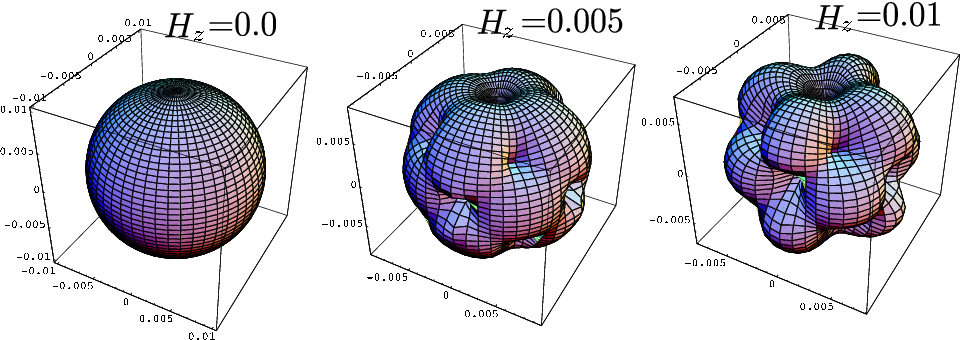
In the following, the spherical Fermi surface, $\varepsilon_{k}=k^{2}/(2m)-E_{F}$, is assumed for simplicity. In this section, we concentrate on the effects of the Zeeman interaction, expressed by $-\sum_{k,\sigma\sigma^{\prime}}\mu_{\rm B}\mbox{\boldmath$H$}\cdot\mbox{\boldmath$\sigma$}_{\sigma\sigma^{\prime}}c^{\dagger}_{k\sigma}c_{k\sigma^{\prime}}$ with $\mbox{\boldmath$H$}=(0,0,H_{z})$, leaving the analysis of the orbital depairing effect until the next sections. When the Zeeman term is added to the Hamiltonian (2), the magnetic field induces the pairing between electrons on the SO split different bands, which gives rise to the Pauli depairing effect. The important observation is that in the case of $E_{\rm SO}\sim\Delta$, Cooper pairs with $k$ for which the spin degeneracy is not lifted by the SO interaction are more seriously affected by the Pauli depairing effect than electron pairs in the strongly SO split regions, leading to the anisotropic Pauli depairing in the momentum space. The anisotropic Zeeman effect in the strongly noncentrosymmetric case has already been discussed by several authors.sam1; mine The unique point in the weakly noncentrosymmetric case is that this effect drastically changes the structure of low-energy excitations in the SC state, and yields the point-node-like structure of the single-particle excitation gap even in isotropic $s$-wave states. To demonstrate this, we calculate the single-particle excitation energy $E_{k\mu}$ ($\mu=1,2,3,4$) by diagonalizing the above mean field Hamiltonian (2) with the Zeeman term expressed in the $4\times 4$ matrix form in the space spanned by the basis $(c^{\dagger}_{k\uparrow},c_{-k\uparrow},c^{\dagger}_{k\downarrow},c_{-k\downarrow})$. The explicit expressions for $E_{k\mu}$ are given in Appendix A. In FIG.1, we depict the numerically calculated single-particle excitation energy gap $E_{\rm gap}$ for the band $\varepsilon_{k-}\equiv\varepsilon_{k}-|\alpha\mbox{\boldmath$\mathcal{L}$}_{0}(\mbox{\boldmath$k$})-\mu_{\rm B}\mbox{\boldmath$H$}|$ in the case with $\Delta/E_{\rm F}=0.01$, and $\alpha/E_{\rm F}=0.03$. Here $E_{\rm gap}$ is defined by the magnitude of $E_{k3}$ for $k$ on the Fermi surface satisfying $\varepsilon_{k-}=0$. It is seen that the point node-like structure develops, as the magnetic field increases. As a matter of fact, the excitation energy $E_{k\mu}$ is not truely gapless, but the excitation energy gap $E_{\rm gap}$ is strongly anisotropic with the structure similar to the point nodes, reflecting the $k$-dependence of the SO term even when the superconducting gap $\Delta$ is independent of $k$. For instance, the excitation energy gaps $E_{\rm gap}$ for $\mbox{\boldmath$k$}_{F}\parallel(001)$, $\mbox{\boldmath$k$}_{F}\parallel(111)$ and $\mbox{\boldmath$k$}_{F}\parallel(100)$ (equivalent to $\mbox{\boldmath$k$}_{F}\parallel(010)$) are equal, and given by,

while for $\mbox{\boldmath$k$}_{F}\parallel(110)$,

with $f(H_{z})=2\alpha^{2}k_{F}^{6}+\mu_{\rm B}^{2}H_{z}^{2}$. It is easily checked that $E_{\rm gap}^{(110)}>E_{\rm gap}^{(001)}$. The positions of the gap minima coincide approximately with the zero points of $\mbox{\boldmath$\mathcal{L}$}_{0}(\mbox{\boldmath$k$})$ at which the SO splitting vanishes. The quasi-particle excitations for $\mbox{\boldmath$k$}_{F}\parallel(001)$, $(111)$, and $(100)$ behave like Dirac fermions with mass gap given by eq.(4). It should be stressed that in the situation considered here the single-particle energy gap $E_{\rm gap}$ does not coincide with the superconducting gap $\Delta$, which is $k$-independent. A similar anisotropic structure of the excitation gap also appears for the band $\varepsilon_{k+}\equiv\varepsilon_{k}+|\alpha\mbox{\boldmath$\mathcal{L}$}_{0}(\mbox{\boldmath$k$})-\mu_{\rm B}\mbox{\boldmath$H$}|$.

Although we use the Dresselhaus interaction in the present calculation, the point-node-like structure appears generally for any forms of $\mbox{\boldmath$\mathcal{L}$}_{0}(\mbox{\boldmath$k$})$ which possess zero points on the Fermi surface.

The anisotroppic Pauli depairing effect discussed in the previous section is particularly important in type II superconductors. Thus, in the following, we consider the orbital depairing effect as well as the Pauli depairing effect on the basis of the quasiclassical analysis. For this purpose, we consider the Green functions for quasiparticles defined on the SO split bands, $G^{(\mu\nu)}(x,x^{\prime})=-\langle T_{\tau}\psi_{\mu}(x)\psi^{\dagger}_{\nu}(x^{\prime})\rangle$, and $F^{(\mu\nu)}(x,x^{\prime})=-\langle T_{\tau}\psi^{\dagger}_{\mu}(x)\psi^{\dagger}_{\nu}(x^{\prime})\rangle$ where $\psi_{\mu}(x)$, $\psi^{\dagger}_{\mu}(x)$ are the field operators for quasiparticles in the $\mu$-band corresponding to the energy in the normal state $\varepsilon_{k\mu}=\varepsilon_{k}+\mu\alpha|\mbox{\boldmath$\mathcal{L}$}_{0}(\mbox{\boldmath$k$})|$ with $\mu=\pm$.com As mentioned above, the inter-band Green functions plays important roles in addition to the intra-band Green functions. Fourier transforming $G^{(\mu\nu)}$ and $F^{(\mu\nu)}$, we introduce the quasiclassical Green functions defined by

with $g^{(\mu\nu)}(\hat{k},\mbox{\boldmath$r$},\varepsilon_{n})=\int\frac{d\varepsilon_{k}}{\pi}G^{(\mu\nu)}(\mbox{\boldmath$k$},\mbox{\boldmath$r$},\varepsilon_{n})$, $f^{(\mu\nu)}(\hat{k},\mbox{\boldmath$r$},\varepsilon_{n})=\int\frac{d\varepsilon_{k}}{\pi}F^{(\mu\nu)}(\mbox{\boldmath$k$},\mbox{\boldmath$r$},\varepsilon_{n})$, and $\bar{g}^{(\mu\nu)}=g^{(\mu\nu)}(-k,\mbox{\boldmath$r$},-\varepsilon_{n})$. Here $k$ is the momentum conjugate to the relative coordinate $\mbox{\boldmath$x$}-\mbox{\boldmath$x$}^{\prime}$, $r$ is the center of mass coordinate, $\hat{k}$ is a unit vector parametrizing the direction of momentum $k$, and $\varepsilon_{n}$ is the fermionic Matsubara frequency. Hereafter, matrices $\breve{A}$ represent $2\times 2$ matrices defined in the space spanned by the basis $(\psi_{\mu},\psi^{\dagger}_{\nu})$ where $\mu=\nu=\pm$ or $\mu=-\nu=\pm$, and matrices $\tilde{B}$ represent those in the two-dimensional space spanned by the band indices $+,-$. Using the standard method,eil; lo; vec we find that $\hat{\mathcal{G}}$ satisfies the Eilenberger equation in the clean limit,

where $\omega=2i\varepsilon_{n}+\mbox{\boldmath$v$}\cdot\frac{2e}{c}\mbox{\boldmath$A$}$ with $A$ a vector potential, and $\tau^{z}=\tilde{1}\otimes\breve{\sigma}^{z}$. The $4\times 4$ matrix $\hat{M}$ is defined by $\hat{M}(\hat{k})=\tilde{\sigma}^{z}\otimes(\alpha\breve{L}(\hat{k}))$, where $\breve{L}(\hat{k})=\breve{1}(|\mbox{\boldmath$\mathcal{L}$}(\hat{k})|+|\mbox{\boldmath$\mathcal{L}$}(-\hat{k})|)/2+\breve{\sigma}^{z}(|\mbox{\boldmath$\mathcal{L}$}(\hat{k})|-|\mbox{\boldmath$\mathcal{L}$}(-\hat{k})|)/2$, and $\alpha|\mbox{\boldmath$\mathcal{L}$}(\hat{k})|=|\alpha\mbox{\boldmath$\mathcal{L}$}_{0}(\hat{k})-\mu_{\rm B}\mbox{\boldmath$H$}|$. The matrix gap function $\hat{\Delta}(\hat{k},\mbox{\boldmath$r$})$ is

with $\breve{\Delta}_{\pm}(\hat{k},\mbox{\boldmath$r$})=i\breve{\sigma}_{y}{\rm Re}\Delta_{\pm}(\hat{k},\mbox{\boldmath$r$})+i\breve{\sigma}_{x}{\rm Im}\Delta_{\pm}(\hat{k},\mbox{\boldmath$r$})$, $\breve{\Delta}_{2}(\hat{k},\mbox{\boldmath$r$})=\breve{\sigma}_{x}{\rm Re}\Delta_{2}(\hat{k},\mbox{\boldmath$r$})-\breve{\sigma}_{y}{\rm Im}\Delta_{2}(\hat{k},\mbox{\boldmath$r$})$, $\Delta_{\pm}(\hat{k},\mbox{\boldmath$r$})=\Delta(\mbox{\boldmath$r$})s_{\pm}(\hat{k})$, $\Delta_{2}(\hat{k},\mbox{\boldmath$r$})=\Delta(\mbox{\boldmath$r$})s_{2}(\hat{k})$, and,

where $\xi_{\pm}(\hat{k})=\sqrt{(1\pm\mathcal{L}_{z}(\hat{k})|\mbox{\boldmath$\mathcal{L}$}(\hat{k})|)/2}$, and $\eta_{\pm}(\hat{k})=-(\mathcal{L}_{x}\pm i\mathcal{L}_{y})/\sqrt{\mathcal{L}_{x}^{2}+\mathcal{L}_{y}^{2}}$. Here, we omit the corrections to the Fermi velocity from the SO interaction, which are not important for $E_{\rm SO}/E_{\rm F}\ll 1$. In the case with strong SO interaction $\alpha\gg\Delta$, the contributions from the inter-band Green functions to eq.(11) are negligible, and the two bands are decoupled. This simplified case was previously studied by several authors.haya; haya2

In spite of the complications raised by the existence of both the inter-band and intra-band Green functions, the analytical soutions of (11) based on the Pesch type approximation are possible. In this approach, we assume the Abrikosov lattice solution for $\Delta(\mbox{\boldmath$r$})$ and the uniform magnetic field in the system, and replace the normal Green functions $g^{(\mu\nu)}$, $\bar{g}^{(\mu\nu)}$ with the spatial averages over a unit cell of the vortex lattice, $\langle g^{(\mu\nu)}\rangle$, $\langle\bar{g}^{(\mu\nu)}\rangle$, retaining only the spatial variation of $f^{(\mu\nu)}$ and $f^{(\mu\nu)\dagger}$. Utilizing the normalization condition $\hat{\mathcal{G}}\cdot\hat{\mathcal{G}}=\mbox{\boldmath$1$}$ and the relations ${\rm tr}[\hat{\mathcal{G}}]=0$, $g^{(+-)*}=g^{(-+)}$, which are derived from (11),ref we find that the quasiclassical Green functions are given by the solutions of the coupled algebraic equations,

where $\tilde{\varepsilon}_{n}^{(\mu\nu)}=\varepsilon_{n}+\frac{i\alpha\mu}{2}(|\mbox{\boldmath$\mathcal{L}$}|-\nu|\mbox{\boldmath$\mathcal{L}^{\prime}$}|)$, $\mbox{\boldmath$\mathcal{L}^{\prime}$}=\mbox{\boldmath$\mathcal{L}$}(-\hat{k})$, $P(\varepsilon)=\frac{1}{2}\partial Y(\varepsilon)/\partial\varepsilon$, $Y(\tilde{\varepsilon}_{n})=\sqrt{\pi}\Delta^{2}u_{n}W(2iu_{n}\tilde{\varepsilon}_{n})$ with $\Delta^{2}=\langle\Delta^{2}(\mbox{\boldmath$r$})\rangle$, $W(z)=e^{-z^{2}}{\rm erfc}(-iz)$, and $u_{n}=\Lambda~{\rm sgn}\varepsilon_{n}/v\sin\theta$ with $\Lambda=\sqrt{\hbar c/2eH_{z}}$ and $\theta$ the polar angle of $\hat{k}$, and $C=2is_{2}s_{+}\alpha|\mbox{\boldmath$\mathcal{L}^{\prime}$}|/\tilde{D}$ with

Since the explicit expressions of the solutions are lengthy, we will present them in Appendix B, and, instead, concentrate on the discussion on the results obtained from them in the following section.

Using the analytical solutions for $\hat{\mathcal{G}}$, we calculate the specific heat and the density of states of quasiparticles. For this purpose, we determine the field-dependence and the temperature-dependence of the spatially averaged gap function $\Delta(H_{z},T)=\sqrt{\langle\Delta^{2}(\mbox{\boldmath$r$})\rangle}$, by solving the quasiclassical BCS gap equation,

where $\bar{\xi}_{\alpha}\equiv\xi_{\alpha}(-\hat{k})$. $\lambda_{0}$ is a dimensionless coupling constant. To compare our calculated results with the experimental observations for Y₂C₃ later, we tune the values of $\lambda_{0}$ and the cutoff for the frequency sum $\varepsilon_{c}$ so as to realize $T_{c}=18$ K. (e.g. $\lambda_{0}=0.2703$, $\varepsilon_{c}=700$ K.) In this calculation, an important parameter is $a_{0}\equiv\sqrt{\mu_{\rm B}\hbar c/(2e\Delta_{0})}/(\pi\xi_{0})$, which is an inverse of the coherence length $\xi_{0}$ normalized to be dimensionless. Here $\Delta_{0}$ is the gap function for $H_{z}=0$. For Y₂C₃, $a_{0}\approx 0.234$. The specific heat in the SC state is

where the density of states for quasiparticles $D_{S}(\varepsilon)$ is given by $D_{S}(\varepsilon)=D_{N}(0)\sum_{\hat{k}}\sum_{\mu=\pm}{\rm Im}\langle g^{(\mu\mu)}(\hat{k},\mbox{\boldmath$r$},\varepsilon+i\delta)\rangle,$ with $D_{N}(0)$ the density of states in the normal state. In FIG.2, we present the calculated results of the specific heat as a function of the normalized magnetic field $h=\mu_{\rm B}H_{z}/\Delta_{0}$ for the temperature $T/T_{c}=0.1$ and several sets of the parameters $\alpha/\Delta_{0}$ and $a_{0}$. It is found that in contrast to the case with strongly broken IS where the SC state is quite robust against the Pauli depairing effect, in weakly noncentrosymmetric systems more low-energy excitations are induced by the magnetic field than in the case with inversion symmetry $\alpha=0$. We interpret the origin of this behavior as the existence of the field-induced nodal excitations mentioned above. The emergence of the point-node-like excitations is more clearly observed in the energy-dependence of the density of states for quasiparticles, which is plotted in FIG.3 for $\alpha/\Delta_{0}=1.0$. As the magnetic field increases, the density of states exhibits the power-law behavior $D_{s}(\varepsilon)\propto\varepsilon^{2}$.

When the SO coupling $\alpha$ is sufficiently smaller than $\Delta_{0}$, another remarkable feature appears in the field-dependence of the specific heat. As shown in FIG.4, for the low magnetic fields $h\approx 0.1\sim 0.2$, a shoulder-like structure of $C_{S}(H_{z})$ similar to a two-gap behavior appears, though there is only a single SC gap $\Delta(\mbox{\boldmath$r$})$. The origin of this behavior is understood as follows. For $\alpha<\Delta_{0}$, there are two different types of the Pauli depairing effect; i.e. (i) one due to the generation of the inter-band pairing correlation which, instead, suppresses the intra-band pairing, and (ii) the other caused by the asymmetric deformation of the Fermi surface. The former is analogous to the usual Pauli depairing effect in centrosymmetric superconductors. The latter effect is inherent in noncentrosymmetric systems. The crucial point is that although the former exists for any finite magnetic fields, the latter is effective only for small fields $\mu_{\rm B}H_{z}<\alpha$, and is suppressed for larger fields $\mu_{\rm B}H_{z}>\alpha$. As a result, the character of the Pauli depairing effect changes around $H_{z}\sim\alpha/\mu_{\rm B}$ in the case of $\alpha<\Delta_{0}$, yielding the shoulder structure of the specific heat coefficient as demonstrated in FIG.4. We would like to stress that this effect is caused by the momentum dependent spin orientatin of Cooper pairs characterizing parity violation. Three remarks are in order. (1) For sufficiently small $\alpha$, e.g. $\alpha=0.05$, $C_{S}$ exhibits a hump rather than a shoulder, in marked contrast with conventional two-gap behaviors. (2) As $\alpha$ increases, the position of the shoulder shifts to larger $h$ regions, though its structure becomes obscure since the orbital depairing effect dominates for high magnetic fields. (3) It should be cautioned that the Pesch approximation is not valid for magnetic fields much lower than $H_{c2}$.vec; pes However, the shoulder structure of $C_{S}$ at $h\sim 0.1$ stems from the Zeeman effect rather than orbital depairing effects. Thus, the above results are applicable to systems with a sufficiently large value of the Ginzburg-Landau parameter $\kappa$, where small magnetic fields can penetrate deeply into the SC regions.

We, now, discuss the implication of the above results for the experimental observations of the weakly noncentrosymmetric superconductor Y₂C₃. This system is almost in the London limit with $\kappa>10$.aki1; aku1 According to the recent LDA calculation, the averaged magnitude of the SO band splitting is roughly $\sim 0.01$ eV,nis which is of the same order as the SC gap $\sim 30$ K.aku1 Thus, our analysis is applicable. A remarkable experimental observation for Y₂C₃ is that the field-dependence of the specific heat exhibits a small shoulder structure for $H_{z}\sim 8\approx H_{c2}/3$ T at $T=2.6$ K.aku2 Although this behavior was interpreted as the indication of the existence of two SC gaps with different magnitudes,aki2; aku2 it can be also, alternatively, explained by assuming the realization of the unique effect associated with parity violation as demonstrated in FIG. 4. A possible test for our scenario is to investigate the field dependence of the nuclear spin relaxation rate,aki2 which should exhibit a gap energy scale different from that observed in the specific heat.

We have shown that in weakly noncentrosymmetric superconductors the Pauli depairing effect is anisotropic in the momentum space, inducing the point-node-like structure of the quasi-particle excitation energy gap even in isotropic $s$-wave states. This effect is caused by the competition between the asymmetric SO interaction and the Zeeman magnetic field in the superconducting state, and yields unique low temperature behaviors of thermodynamic quantities quite different from those of conventional $s$-wave superconductors. Also, by using the quasiclassical method, we have demonstrated that the magnetic field dependence of the specific heat exhibits a multi-gap-like structure for sufficiently small SO interaction even when there is only a single gap. These effects are associated with the momentum-dependent spin orientation of Cooper pairs which characterizes parity violation. Thus, our results reveal the unique aspects of parity violated Cooper pairs inherent in weakly noncentrosymmetric systems. We have also discussed that our findings may be relevant to the recent experimental observations for Y₂C₃.

References

- (1) E. Bauer, G. Hilscher, H. Michor, Ch. Paul, E. W. Scheidt, A. Gribanov, Yu. Seropegin, H. Noël, M. Sigrist, and P. Rogl, Phys. Rev. Lett. 92, 027003 (2004).
- (2) N. Kimura, K. Ito, K. Saitoh, Y. Umeda, H. Aoki, and T. Terashima, Phys. Rev. Lett. 95, 247004 (2005).
- (3) I. Sugitani, Y. Okuda, H. Shishido, T. Yamada, A. Thamizhavel, E. Yamamoto, T. D. Matsuda, Y. Haga, T. Takeuchi, R. Settai, and Y. Onuki, J. Phys. Soc. Jpn. 75, 043703 (2006).
- (4) T. Akazawa, H. Hidaka, H. Kotegawa, T. Kobayashi, T. Fujiwara, E. Yamamoto, Y. Haga, R. Settai, and Y. nuki, J. Phys. Soc. Jpn. 73, 3129 (2004).
- (5) K. Togano, P. Badica, Y. Nakamori, S. Orimo, H. Takeya, and K. Hirata, Phys. Rev. Lett. 93, 247004 (2004).
- (6) V. M. Edelstein, Sov. Phys. JETP 68, 1244 (1989).
- (7) V. M. Edelstein, Phys. Rev. Lett. 75, 2004 (1995).
- (8) L. P. Gor’kov and E. Rashba, Phys. Rev. Lett. 87, 037004 (2001).
- (9) P. A. Frigeri, D. F. Agterberg, A. Koga, and M. Sigrist, Phys. Rev. Lett. 92, 097001 (2004).
- (10) K. Samokhin, Phys. Rev. Lett.94 027004 (2005).
- (11) I. A. Sergienko and S. H. Curnoe, Phys. Rev. B70, 214510 (2004).
- (12) S. K. Yip, Phys. Rev. B 65, 144508 (2002).
- (13) K. Samokhin, Phys. Rev. B70, 104521 (2004).
- (14) V. Barzykin and L. P. Gorkov, Phys. Rev. Lett. 89, 227002 (2002).
- (15) O. V. Dimitrova and M V. Feigel’man, JETP letters 78, 637 (2003).
- (16) R. P. Kaur, D. F. Agterberg, and M. Sigrist, Phys. Rev. Lett.94, 137002 (2005).
- (17) V. P. Mineev, Phys. Rev. B71, 012509 (2005).
- (18) S. Fujimoto, Phys. Rev. B72, 024515 (2005).
- (19) S. Fujimoto, J. Phys. Soc. Jpn. 76, 034712 (2007).
- (20) S. Fujimoto, J. Phys. Soc. Jpn. 76, 051008 (2007).
- (21) N. Hayashi, K. Wakabayashi, P.A. Frigeri, and M. Sigrist, Phys. Rev. B73, 092508; ibid 73, 024504 (2006).
- (22) Y. Nagai, Y. Kato, and N. Hayashi, J. Phys. Soc. Jpn. 75, 043706 (2006).
- (23) G. Eilenberger, Z. Phys. 214, 195 (1968),
- (24) A. I. Larkin and Y. N. Ovchinnikov, Sov. Phys. JETP 28, 1200 (1969).
- (25) G. Amano, S. Akutagawa, T. Muranaka, Y. Zenitani, and J. Akimitsu, J. Phys. Soc. Jpn. 73, 530 (2004).
- (26) A. Harada, S. Akutagawa, Y. Miyamichi, H. Mukuda, Y. Kitaoka, and J. Akimitsu, J. Phys. Soc. Jpn. 76, 023704 (2007).
- (27) S. Akutagawa and J. Akimitsu, J. Phys. Soc. Jpn. 76, 024713 (2007).
- (28) S. Akutagawa, T. Ohashi, H. Kitano, A. Maeda, J. Goryo, H. Matsukawa, and J. Akimitsu, unpublished.
- (29) I. A. Sergienko, Physica B359-361 581 (2005).
- (30) Y. Nishikayama, T. Shishidou and T. Oguchi, J. Phys. Soc. Jpn.76, 064714 (2007).
- (31) G. Dresselhaus, Phys. Rev. 100, 580 (1955).
- (32) In the derivation of the Gor’kov equations for and , we use the fact that the momentum which appears in the unitary transformation from the basis of () to the basis of () commutes with the center of mass coordinate in the quasiclassical method.
- (33) I. Vekhter and A. Houghton, Phys. Rev. Lett. 83, 4626 (1999); Phys. Rev. B57, 10831 (1998).
- (34) W. Pesch, Z. Phys. B21, 263 (1975).
- (35) Because of the Zeeman effect, the particle-hole symmetry is broken, i.e. . This property of the Zeeman field is also noticed in ref.haya and ere.
- (36) I Eremin and J. F. Annett, Phys. Rev. B74, 184524 (2006).