Decentralized Sequential Change Detection Using Physical Layer Fusion

$X\sim\mathcal{N}(\theta,\sigma^{2})$ indicates that $X$ is a Gaussian random variable with mean $\theta$ and variance $\sigma^{2}$.

(1) The state of nature is described by $\left\{\theta_{k}:k\in\mathbb{Z}_{+}\right\}$, a two-state discrete-time Markov chain taking values in $\{m_{0},m_{1}\}$, with transition probabilities as described in Fig. 1(a)-(b). The quantities $m_{0}$ and $m_{1}$ denote, for example, the mean level of the observations before and after the disruption. The initial distribution for this Markov chain is obtained from $\Pr\{\theta_{0}=m_{1}\}=\nu$. The change time $\Gamma$ is $\mathbb{Z}_{+}$-valued, and given the event $\{\Gamma>0\}$, $\Gamma$ has the geometric distribution.

(2) The network has $L$ sensors. At time $k$, sensor $S_{l}$ makes an observation $X_{l,k}\sim\mathcal{N}(\theta_{k},\sigma_{\textsf{obs},l}^{2})$, i.e., $X_{l,k}=\theta_{k}+Z_{l,k},$ where $Z_{l,k}\sim\mathcal{N}(0,\sigma_{\textsf{obs},l}^{2}),l=1,\ldots,L$.

(3) The observations at each sensor are independent, conditioned on $\theta_{k}$. Furthermore, the observations are independent from sensor to sensor, conditioned on $\theta_{k}$. Despite these conditional independence assumptions, we remark that $X_{l,k},l=1,\ldots L$, are correlated.

(4) Each sensor transmits $Y_{l,k}=\phi_{l,k}(X_{l,k})$; this being a function only of the observation at sensor $l$, our setting is a decentralized one. See Fig. 1(c). The function $\phi_{l,k}$ is affine:

Quantities $\alpha_{k}=(\alpha_{1,k},\ldots,\alpha_{L,k})$ and $c_{k}=(c_{1,k},\ldots,c_{L,k})$ are parameters for optimal control. Transmission is done by setting the amplitude of an underlying unit-energy waveform to $Y_{l,k}$. All sensors use the same underlying waveform. The motivations for the analog amplify-and-forward transmissions in (1) are given in Section I: conditional independence of the observations given the state, and the Gaussian observation noise. If the latter does not hold, affine functions of LLRs instead of the direct observations could be sent ([21, Ch. 5]).

(5) The GMAC output at the fusion center when projected onto the common waveform yields

where $Z_{\textsf{MAC},k}\sim\mathcal{N}(0,\sigma_{\textsf{MAC}}^{2})$ is independent and identically distributed (iid) across $k$, and is independent of all other quantities. The gain $h_{l}\in\mathbb{R}_{+}$ is the channel gain for the $l$th sensor and is deterministic. See Fig. 1(c). We assume perfect knowledge of the channel gains is available at the sensors and the fusion center. While this is not the case in practice, channel knowledge can be gleaned in time-division duplex (TDD) systems that possess channel reciprocity (IEEE 802.15.4). See Mudumbai, Barriac & Madhow [1] for a suggested master-slave architecture. In a subsequent section, we study the effect of imperfect knowledge of these gains.

(6) At the fusion center, form $\widehat{Y}_{k}$ as follows:

where $\widehat{Z}_{\textsf{MAC},k}\sim\mathcal{N}(0,\sigma_{k}^{2})$ and

The quantity $\widehat{Y}_{k}$ in (2) is obtained from $\widetilde{Y}_{k}$ using a bijective mapping; so no information is lost. From (2), we also see that the distributed multi-sensor setting is equivalent to a centralized setting where the fusion center makes a direct (noisy) observation on $\theta_{k}$ with equivalent additive observation noise of variance $\sigma_{k}^{2}$ as given in (3). This is enabled by the affine nature of $\phi_{l,k}$. The centralized problem with constant $\sigma_{k}^{2}$ was studied by Shiryayev [5] with the aim of characterizing the stopping rule. The new aspect here is the dependence of $\sigma^{2}_{k}$ on the control parameters.

(7) The fusion center chooses an action $a_{k-1}\in\mathbb{A}$ at time $k-1$ from set $\mathbb{A}$ of actions (controls)

If $a_{k-1}=stop$, the fusion center stops. If $a_{k-1}=(continue,\alpha_{k},c_{k})$, the fusion center takes another sample (the $k$th), and all sensors transmit $\phi_{l,k}(X_{l,k})$ with parameters $(\alpha_{k},c_{k})$.

(8) As done by Veeravalli in [8], we assume a quasi-classical information structure, i.e., action $a_{k-1}$ depends on

Even though the sensors may have local memory of past observations, our framework does not make use of this additional information.⁴⁴ 4 Veeravalli [8, p.434] discusses other information structures and why they may be difficult to analyze. The fusion center feeds back the action parameters $a_{k-1}$ to the sensors. (We use the following notation: the quantity $i_{k-1}$ in (4) is a realization of the random variable $I_{k-1}$ and takes values in the set $\mathbb{I}_{k-1}$. We set $\mathbb{I}_{0}=\emptyset$).

(9) Average power constraint at sensor $l$ is

i.e.,

The set of feasible controls, given $I_{k-1}=i_{k-1}$, is denoted by

In Section III, we relax the constraint in (5) and impose an expected total energy constraint.

(10) The fusion center policy $\pi$ is a sequence of proposed (deterministic) actions $\pi=(\pi_{k-1},k\geq 1)$, where $\pi_{k-1}$ is a function $\pi_{k-1}:\mathbb{I}_{k-1}\rightarrow\mathbb{A}$. In particular, $\pi_{k-1}(i_{k-1})=a_{k-1}\in\mathbb{A}(i_{k-1})$. Each policy $\pi$ induces a probability measure. All expectations are with respect to this measure. The dependence of the expectation operation on $\pi$ is understood and suppressed.

(11) $\tau$ is the first instant when the fusion center decides to stop.

The problem we wish to solve is the following:

The solution to Problem 1 is obtained via a solution to Problem 2 (below) for a particular $\lambda>0$ (Shiryayev [5]). The quantity $\lambda$ may be interpreted as the cost of unit delay.

The cost function is additive over time. The first term within the expectation in (7) is the terminal cost; the terms in the summation a running cost. At each stage the state $\theta_{k}$ evolves in a Markov fashion. The controller sees only a noisy version $\widehat{Y}_{k}$ of the state, but can control the observation noise variance $\sigma_{k}^{2}$ via $\alpha$ and $c$. It can also stop at any stage and pay a terminal cost. Any decision affects the future evolution of the cost process. Such problems are Markov decision problems (MDP) with partial observations. They can be analyzed by studying an equivalent complete observation MDP⁵⁵ 5 See Shiryayev [5], Veeravalli [6] for results with stopping, Bertsekas & Shreve [22, Ch. 10] for discounted costs, and Bertsekas [23, Ch. V]. with a reduced (posterior) state $\mu_{k}\stackrel{{\scriptstyle\Delta}}{{=}}\mathbb{E}\left[1\{\theta_{k}=m_{1}\}\mid I_{k}\right]=\Pr\{\Gamma\leq k\mid I_{k}\}.$ The probability law for $\{\mu_{k}:k\geq 0\}$ is given as follows: $\mu_{0}=\Pr\{\Gamma\leq 0\mid I_{0}\}=\nu$, and the law for $\mu_{k}$, under $a_{k}=(continue,\alpha_{k+1},c_{k+1})$, is (see Veeravalli [6, eqn. (9)])

where $\beta_{k}\stackrel{{\scriptstyle\triangle}}{{=}}\Pr\{\Gamma\leq k+1|I_{k}\}=\mu_{k}+(1-\mu_{k})p$, and $f_{m_{i},\alpha_{k+1}}$ is the density of an $\mathcal{N}(m_{i},\sigma_{k+1}^{2})$ random variable. The quantities $h$ and $g$ are as in (8); $h$ is the density of $\hat{Y}_{k+1}$ given $(I_{k},a_{k})$, and $g$ is a scaled density. The power constraint (5) when written for time $k+1$ simplifies to

The set of feasible controls in (6) depends on $i_{k}$ only through $\mu_{k}$ and can be simplified to

where $\mathbb{A}(\cdot)$ is re-used to denote the set of feasible controls for the equivalent complete observation MDP. Let $\mathbb{A}^{\prime}(\mu)=\{(\alpha,c):(continue,\alpha,c)\in\mathbb{A}(\mu)\}$ denote the set of control parameters when the action is to continue. Now consider the objective function. Taking conditional expectations with respect to the information process, (see Shiryayev [5, pp.195–196]), (7) reduces to

Minimization of (10) is done via dynamic programming. Some additional remarks are in order.

Remarks: 1. The variance $\sigma_{k+1}^{2}$ depends on $\alpha_{k+1}$ as shown in (3), and hence the dependence on $\alpha_{k+1}$ in (8). $\mu_{k+1}$ depends on $c_{k+1}$ only through $\alpha_{k+1}$ because of the processing done in (2).

2. If the running cost is $\lambda$ instead of $\lambda 1\{\theta_{k}=m_{1}\}$ in (7), every sample costs $\lambda$ units, not just those beyond the change point that contribute to the delay. This is a minor variation to Problem 2 and has a similar solution.

3. Another variation is sequential hypothesis testing: set the transition probability $p=0$, enhance the action $stop$ to $(stop,\hat{\theta})$, where $\hat{\theta}$ is the decision (either $m_{0}$ or $m_{1}$), and set the terminal cost to $1\{\theta_{\tau}\neq\hat{\theta}\}$. The running cost is a constant $\lambda$ for every sample.

As is usual with such problems, we first restrict the stopping time $\tau$ to a finite horizon $T$. Using Bertsekas’s result [23, Ch.1, Prop.3.1], the cost-to-go function recursions are written as

To solve Problem 2, let $T\rightarrow\infty$. From results in [8] and [6], the limit in (11) below exists, does not depend on $k$ (i.e., the policy is stationary), and defines the infinite horizon cost-to-go function:

where

The following lemma enables a characterization of the optimal stopping policy.

The proof is the same as that in Bertsekas [23, p. 268] for sequential hypothesis testing. The concavity of $A_{J}(\mu)$ and (11) imply the following theorem (Shiryayev [5], Veeravalli [6]).

To summarize, the optimal detection strategy at time $k$ is as follows. Convert the received signal $\tilde{Y}_{k}$ into the posterior probability of change $\mu_{k}$ using (2) and (8). If $\mu_{k}$ exceeds a threshold, declare that a change has occurred. Otherwise, make the sensors transmit another sample using parameters $\alpha,c$ chosen optimally as described in the next subsection.

We begin this section with an algorithm that calculates the optimal $\alpha$.

The optimal choice sets amplitudes of the $k$ sensors with the $k$ least scaled observation noise variance ($\sigma_{\textsf{obs},l}^{2}h_{l}\alpha_{\max,l}$) to $\alpha_{\textsf{max},l}$. The remaining sensors’ amplitudes are appropriately chosen smaller values. Intuitively, sensors $l=k+1,\ldots,L$ have so good a channel that scaling by $\alpha_{\textsf{max},l}$ for these sensors will amplify the observation noise leading to a larger overall noise variance. Note that when all channel gains, observation variances, and power constraints are equal, $\alpha_{l}=\alpha_{\textsf{max}}$ for all sensors. This special case was earlier proved in [24].

Let us now restrict the controls to be of the following form: the decision to stop or continue, say $b_{k}$, depends on $I_{k}$, but the parameters of the affine transformation at time $k+1$ can only depend on $I_{0}$ and $b_{k}\in\{stop,continue\}$. $I_{0}$ denotes the prior information before any observations are made and $b_{k}$ is the decision of the fusion center at $k$. Note that this reduces the amount of feedback to simply the binary random variable $b_{k}$.

The structure of the controls is similar to that of the optimal policy of the previous section, but with

so that $(\alpha,c)$ depends on only $I_{0}$ and not on $I_{k}$. The stopping policy is chosen as in Theorem 2. As we see in simulation results presented in Section IV, the performance of this algorithm is close to optimal for the chosen parameters, yet requires feedback of only one bit at each stage.

Veeravalli [6] addresses the structure of optimal $D_{l}$-level quantizer at sensor $S_{l},l=1,2,\ldots,L$. His model is applicable to a system that allows $\log_{2}D_{l}$ bits to be sent error-free from sensor $S_{l}$ to the fusion center. For simplicity let $D_{l}=D,l=1,2,\ldots,L$. In order to show the benefit of exploiting correlation of observations when transmitting across the GMAC, we do the following. The quantized bits from the sensors in Veeravalli’s scheme are transmitted using an optimal scheme designed for independent data streams over a coherent GMAC. If all sensors operate at the same transmission power, the SNR required to support such a transmission on the GMAC satisfies the sum rate constraint $L\log_{2}{D}\leq(1/2)\log_{2}{\left(1+L\cdot\textsf{SNR}\right)},$ and thus

For the simulations, we assume two sensors ($L=2$) with equal gains, i.e., $h_{l}=1$ for $l=1,2$. We also assume one-bit quantizers ($D=2$). From (20) we get $\textsf{SNR}\geq 7.5$. Algorithms operate at $\textsf{SNR}=7.5$ with $P_{l}=7.5$ for $l=1,2$ and $\sigma_{\textsf{MAC}}^{2}=1$. We now summarize the other simulation assumptions which will be used unless stated otherwise.

Fig. 3 shows that both our algorithms give lesser delays than Veeravalli’s algorithm that is naively overlaid on the GMAC. Furthermore, the suboptimal policy of Section II-D degrades from that in Section II-B only for low false alarm probabilities.

In Veeravalli’s algorithm, $D-1$ thresholds ($\in\mathbb{R}^{D-1}$) and a decision to stop or continue are fed back to each sensor. Our scheme requires feedback of $\alpha_{l}\in\mathbb{R}_{+},c_{l}\in\mathbb{R}$, and the binary decision. Even simpler is the strategy in Section II-D; only a binary decision is fed back.

The network delay is independent of the number of sensors in both our algorithms; the performance improves with increasing number of sensors. Veeravalli’s scheme on the other hand requires an exponential growth in SNR (with $L$, as in (20)) to maintain the same delay versus $P_{\textsf{FA}}$ performance. Our algorithms need a higher level of time and frequency synchronization of the transmitters for beamforming. Section IV-D studies the effect of lack of perfect channel knowledge. Transmit beamforming can be achieved via uplink-downlink reciprocity in a static time-division duplex (TDD) system (see [1] for an example mechanism).

We now portray performance under three different settings.

• •

  Fig. 4 shows performance for various channel SNRs $P/\sigma_{\textsf{MAC}}^{2}$; the other parameters remain as in Simulation Setup 1.

• •

  Fig. 5 shows performance for various observation SNRs $(m_{1}-m_{0})^{2}/\sigma_{\textsf{obs}}^{2}$ when the channel SNR $P/\sigma_{\textsf{MAC}}^{2}$ is fixed at 3 dB.

• •

  Fig. 6 compares the symmetric and asymmetric channel gain cases. The symmetric curve is obtained with $h_{l}=1$ for $l=1,2$, and the asymmetric one with $h_{1}=1$ and $h_{2}=0.75$. The weaker sensor is 2.5 dB lower than the stronger one.

The plots show graceful degradation with decreasing SNR with results along expected lines.

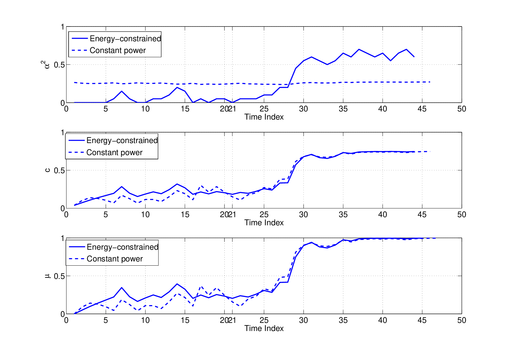
For $P_{\textsf{FA}}\leq e^{-4}$, we first identify the minimum time to detect change as a function of the energy constraint. This yields a power constraint for the constant power formulation. We then compare the delays incurred by the optimal algorithm under the two formulations in Fig. 7. We use the parameters in Simulation Setup 1 and $h_{l}=1$ for all sensors. For the same $P_{\textsf{FA}}$, the energy-constrained solution declares a change with lesser delay than the constant power solution.

As an illustration, we plot in Fig. 8 the variation of $\alpha^{2}$, $c$, and $\mu$ with time in both the algorithms for a representative sample path. The change point is at $21$ samples, shown using a dotted vertical grid line. The energy-constrained solution is more energy efficient because it uses lower energy ($\alpha^{2}$) before and higher energy after the change point. Indeed, based on the prior information, the first few samples use negligible energy.

Thus far we assumed a static channel with perfect knowledge available at both transmitter and receiver. Wireless channels, however, change with time. Only an estimate of the channel, based on signal processing on the pilots, beacons, or preambles, may be available. In this section, we study the effect of imperfect channel knowledge on the physical layer fusion algorithm.

To arrive at a model for channel errors, we consider complex channel gains over the GMAC with noise given by $Z_{\textsf{MAC},k}\sim\mathbb{C}\mathcal{N}(0,\sigma_{\textsf{MAC}}^{2})$, a circular symmetric complex Gaussian random variable. The observations are real-valued, but the complex baseband equivalent signal has two real-valued degrees of freedom per sample, leading to a bandwidth expansion factor of two. Suppose that the sensors use transmit beamforming⁶⁶ 6 The optimality of cooperative transmit beamforming by sensors remains an open question., i.e., $\alpha_{l}=\frac{h_{l}^{*}}{|h_{l}|}\gamma_{l}$. Then it is sufficient to preserve only the real part of the received signal at the fusion center, and the problem reduces to that studied in the earlier parts of this paper with $\sigma_{\textsf{MAC}}^{2}$ replaced by $\sigma_{\textsf{MAC}}^{2}/2$ in Section II. The quantity $\gamma_{l}$ replaces $\alpha_{l}$ and $|h_{l}|$ replaces $h_{l}$ in Algorithm 1. The output of the algorithm is $\gamma_{l}$.

Let $\{h_{l}\}$ be a sequence of $\mathbb{C}\mathcal{N}(0,1)$ random variables that obey a block-fading model, i.e., the channel remains constant for $T$ uses and then changes to an independent channel gain. If $K$ of these $T$ samples are available for channel estimation, then the MMSE estimate of the channel is $\hat{h}_{l}=(h_{l}+rZ)/(1+r^{2})$, where $r=\sigma_{\textsf{MAC}}/\sqrt{KP_{l}}$, $P_{l}$ is the power of sensor $l$ and $Z\sim\mathbb{C}\mathcal{N}(0,1)$. This is estimated at both ends (using TDD system’s channel reciprocity).

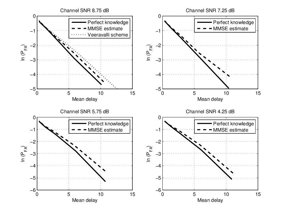
Figures 9 and 10 show performance of the policy of Section II-C with $\hat{h}$ used in place of actual $h$, across different channel SNRs. Simulation Setup 1 parameters are used. $K=1$, i.e., only one sample pilot is used for channel estimation so that transmit beamforming is only loosely enabled. The pilot SNR equals the channel SNR in Fig. 9 and is 8.75 dB lower in Fig. 10. The top-left subplot in Fig. 9 shows that the transmit beamforming scheme with estimation errors is indeed superior to Veeravalli’s scheme on a coherent GMAC. Fig. 10 shows no benefit because the pilot SNR is not sufficient. Other subplots show graceful degradation with decreasing SNR.

References

- [1] R. Mudumbai, G. Barriac, and U. Madhow, “On the feasibility of distributed beamforming in wireless networks,” IEEE Trans. Wireless Commun., vol. 6, no. 5, pp. 1754–1763, May 2007.
- [2] S. M. Ali and S. D. Silvey, “A general class of coefficients of divergence of one distribution from another,” J. Royal Statist. Soc., Ser. B, vol. 28, no. 1, pp. 131–142, 1966.
- [3] E. S. Page, “Continuous inspection schemes,” Biometrika, vol. 41, no. 1/2, pp. 100–115, Jun. 1954.
- [4] G. Lorden, “Procedures for reacting to a change in distribution,” Ann. Math. Statist., vol. 42, pp. 1897–1908, Dec. 1971.
- [5] A. N. Shiryayev, Optimal Stopping Rules. New York: Springer-Verlag, 1978.
- [6] V. V. Veeravalli, “Decentralized quickest change detection,” IEEE Trans. Inform. Theory, vol. 47, no. 4, pp. 1657–1665, May 2001.
- [7] J. N. Tsitsiklis, Advances in Statistical Signal Processing. Greenwich, CT: JAI Press, 1993, vol. 2, ch. Decentralized Detection, pp. 297–344.
- [8] V. V. Veeravalli, T. Başar, and H. V. Poor, “Decentralized sequential detection with a fusion center performing the sequential test,” IEEE Trans. Inform. Theory, vol. 39, no. 2, pp. 433–442, Mar. 1993.
- [9] V. K. Prasanthi, “Towards a cross layer design of sequential change detection over ad hoc wireless sensor networks,” Master’s thesis, Indian Institute of Science, Bangalore, India, June 2006.
- [10] V. K. Prasanthi and A. Kumar, “Optimizing delay in sequential change detection on ad hoc wireless sensor networks,” in Proc. IEEE SECON, Reston, VA, Sep. 2006.
- [11] T. Berger, Rate Distortion Theory: A Mathematical Basis for Data Compression. Englewood Cliffs: Prentice-Hall, 1971.
- [12] A. Lapidoth and S. Tinguely, “Sending a bi-variate Gaussian source over a Gaussian MAC,” in Proc. 2006 IEEE International Symposium on Information theory, Seattle, Washington, Jul. 2006.
- [13] G. Mergen and L.Tong, “Type based estimation over multiaccess channels,” IEEE Trans. Signal Processing, vol. 54, no. 2, pp. 613–626, Feb. 2006.
- [14] G. Mergen, V. Naware, and L. Tong, “Asymptotic detection performance of type-based multiple access over multiaccess fading channels,” IEEE Trans. Signal Processing, vol. 55, no. 3, pp. 1081–1092, Mar. 2007.
- [15] K. Liu and A. M. Sayeed, “Type-based decentralized detection in wireless sensor networks,” IEEE Trans. Signal Processing, vol. 55, no. 5, pp. 1899–1910, May 2007.
- [16] K. Liu, H. E. Gamal, and A. Sayeed, “Decentralized inference over multiple-access channels,” IEEE Trans. Signal Processing, vol. 55, no. 7, pp. 3445–3455, Jul. 2007.
- [17] M. Gastpar and M. Vetterli, “Scaling laws for homogeneous sensor networks,” in Proceedings of the 41st Ann. Allerton Conf. Commun., Contr., Comput., Monticello, IL, Oct. 2003.
- [18] M. Gastpar, B. Rimoldi, and M. Vetterli, “To code, or not to code: Lossy source-channel communication revisited,” IEEE Trans. Inform. Theory, vol. 49, pp. 1147–1158, May 2003.
- [19] M. Gastpar and M. Vetterli, “Power, spatio-temporal bandwidth, and distortion in large sensor networks,” IEEE J. Select. Areas Commun., vol. 23, pp. 745–754, Apr. 2005.
- [20] E. Ertin and L. C. Potter, “Decentralized detection with generalized costs,” in Proc. Second ARL Feder. Lab. Symp., College Park, MD, Feb. 1998.
- [21] L. Zacharias, “Decentralized sequential detection using physical layer fusion,” Master’s thesis, Indian Institute of Science, Bangalore, India, June 2007.
- [22] D. P. Bertsekas and S. E. Shreve, Stochastic Optimal Control: The Discrete Time Case. NY: Academic Press, 1978.
- [23] D. P. Bertsekas, Dynamic Programming and Optimal Control, Volume 1. Massachusetts: Athena Scientific, 1995.
- [24] L. Zacharias and R. Sundaresan, “Decentralized sequential change detection using physical layer fusion,” in Proc. 2007 IEEE Int. Symp. on Inform. Theory, Nice, France, Jun. 2007.
- [25] I. Csiszár, “Information-type measures of difference of probability distributions and indirect observations,” Studia Sci. Math. Hungar., vol. 2, pp. 299–318, 1967.
- [26] A. Padakandla and R. Sundaresan, “Separable convex optimization problems with linear ascending constraints,” Submitted to SIAM J. on Opt. http://arxiv.org/abs/0707.2265, Jul. 2007.