Targeted Excited State Algorithms
Abstract
To overcome the limitations of the traditional state-averaging approaches in excited state calculations, where one solves for and represents all states between the ground state and excited state of interest, we have investigated a number of new excited state algorithms. Building on the work of van der Vorst and Sleijpen (SIAM J. Matrix Anal. Appl., 17, 401 (1996)), we have implemented Harmonic Davidson and State-Averaged Harmonic Davidson algorithms within the context of the Density Matrix Renormalization Group (DMRG). We have assessed their accuracy and stability of convergence in complete active space DMRG calculations on the low-lying excited states in the acenes ranging from naphthalene to pentacene. We find that both algorithms offer increased accuracy over the traditional State-Averaged Davidson approach, and in particular, the State-Averaged Harmonic Davidson algorithm offers an optimal combination of accuracy and stability in convergence.
I Introduction
Many excited states possess complicated electronic structure which cannot be described by a single dominant electronic configuration. For such states, a reliable description requires a multireference quantum chemistry method.
Recently, the Density Matrix Renormalization Group (DMRG) has emerged as a new tool for multireference quantum chemistry problems Yaron et al. 1998; White and Martin 1999; Legeza et al. 2003a; Fano et al. 1998; Shuai et al. 1997; Chan and Head-Gordon 2002; Hallberg 2006. When applied to bond-breaking, it achieves a balanced description across potential energy curves due to its reference-free nature Legeza et al. 2003b; Moritz et al. 2005; Chan et al. 2004. Reduced-scaling DMRG algorithms have also been developed and applied to large multireference problems in quasi-one-dimensional systems such as conjugated polyenes and acenes Hachmann et al. 2006; Hachmann et al. 2007.
The DMRG ansatz can be written as a linear expansion in terms of many-body functions which are subsequently optimised with respect to internal non-linear degrees of freedom ,
| (1) |
Note that if we choose the expansion functions to be Slater determinants and the internal degrees of freedom to be their constituent orbitals, the above ansatz describes the Complete-Active-Space Self-Consistent-Field (CASSCF) wavefunction Roos 1987. In the DMRG, the expansion functions are instead complicated many-body basis states and the non-linear degrees of freedom are renormalisation matrices, which allows for a particularly compact and efficient expansion Schollwöck 2005.
To obtain excited states in the DMRG we usually use the iterative Davidson algorithm to solve for eigenvectors ranging from the ground-state to the excited state of interest Hallberg 2003. The non-linear parameters for these states are subsequently optimised for a density matrix that is averaged over all the states . State-averaging is necessary to improve the stability of the non-linear optimisation and to prevent root-flipping, which occurs when the approximate wavefunction leaves the convergence basin of the target excited state and enters that of a different excited state Docken and Hinze 1972; Khait et al. 1995; Knowles and Werner 1992; Hoffmann et al. 2002; Cancès et al. 2006.
The drawbacks of this conventional approach, which we shall refer to as the State-Averaged Davidson (SA-D) algorithm, become clear if one is interested in higher regions of the spectrum because it becomes infeasible, both in terms of computational cost and accuracy, to solve for and adequately represent all the lower-lying eigenvectors in the state-averaged DMRG basis. Consequently, it is desirable to explore alternative algorithms that directly yield individual or a few excited state wavefunctions at a time. Any such an algorithm should also retain the stability of the SA-D algorithm during non-linear optimisation, so as to be able to rapidly converge to the desired target excited state(s) without root-flipping.
Iterative methods for linear algebra that work with shifted and inverted operators such as have long been used in numerical analysis to obtain the interior (i.e. excited state) eigenvalues of matrices Morgan 1991; Bai et al. 2000. Sleijpen and van der Vorst proposed an efficient modification that used a shifted and inverted operator to directly calculate harmonic Ritz approximations to excited eigenvalues and eigenvectors Sleijpen and van der Vorst 1996. We shall refer to this variant as the Harmonic Davidson (HD) algorithm to distinguish it from the original algorithm above. Aside from a demonstration for the one-electron Kohn-Sham equation in Ref. Tackett and Ventra 2002, we are not aware of the application of this technique elsewhere in quantum chemistry.
The purpose of this work is to investigate the Harmonic Davidson algorithm as a means to directly target individual excited states and regions of the spectrum within the DMRG. One area in which the current application to quantum chemistry differs from previous numerical applications is the presence of a subsequent nonlinear optimisation step for the wavefunction. We investigate how combining the Harmonic Davidson procedure with state-averaging over nearby states in the spectrum (State-Averaged Harmonic Davidson, or SA-HD) can be used to confer stability in this non-linear optimisation. While we have focused on the DMRG method here, our findings are relevant to excited state algorithms for other quantum chemistry methods whose ansatz contains both linear and non-linear parameters, such as in the CASSCF method.
The structure of this paper is as follows. In Sec. II, we briefly review the DMRG method and the Davidson and Harmonic Davidson algorithms. In Sec. III, we present DMRG calculations on the excited states of acenes from naphthalene to pentacene using both direct targeting with the Harmonic Davidson algorithm (in both state-averaged and non-state-averaged forms) as well as with the traditional (state-averaged) Davidson approach. We also compare our excited state spectrum with that obtained from Equation of Motion Coupled Cluster theory. We summarise our findings in Sec. IV.
II Theory
II.1 DMRG
The quantum chemistry DMRG algorithm used in this work has been described fully elsewhere Hachmann et al. 2006; Chan 2004. As a detailed understanding is not necessary here, we shall restrict ourselves to only the essentials. As described above, the DMRG wavefunction may be written in the form (1). The DMRG sweep algorithm then provides an iterative method through which the many-body basis functions may be optimised with respect to a set of internal non-linear parameters . For each orbital in the problem we can associate an matrix, which describes a many-body renormalisation transformation involving the orbital (i.e. not simply an orbital rotation). In a sweep to optimize the states (an analogous procedure holds for the states), matrices are determined from the eigenvectors of the many-particle reduced density matrix with the largest eigenvalues. In the ground-state case, the density matrix that determines the states is obtained by tracing out the states from the wavefunction, viz
| (2) | ||||
| (3) |
is referred to as the size of the DMRG many-body basis, and as increases, the DMRG wavefunction becomes exact. For excited state calculations, it is usual to employ state-averaging to increase the stability of the non-linear optimisation. This consists of using an averaged reduced density matrix in eq. (2)
| (4) |
where typically we choose equal weights for all the states of interest.
II.2 The Davidson Algorithm
The Davidson algorithm provides an efficient iterative solver for the large number of linear coefficients in the expansion of the ground-state DMRG wavefunction (1) Crouzeix et al. 1994; Saad 1993. is expressed in an auxiliary basis (generated by the Davidson iterations)
| (5) | ||||
| (6) |
The coefficients are determined by left-projection with
| (7) |
where is the approximate expectation value . Each iteration of the Davidson algorithm, generates a new basis function from the current trial solution via
| (8) |
which is then orthogonalised against and added to the subspace .
To obtain excited state eigenvectors, the simple generalization known as the block Davidson or Davidson-Liu algorithm Davidson 1975; Olsen et al. 1990 is typically used. Here a residual vector is generated for each of the states from the ground-state up to the target excited state. Solution of the subspace eigenvalue equation (7) then yields successive approximations to all eigenstates up to the excited state of interest. In the subsequent non-linear optimisation of the excited state in the DMRG algorithm, the eigenvectors obtained from the block Davidson algorithm (i.e. from the ground-state to the target eigenvector of interest) are all averaged together in the density matrix (4). We shall refer to this combined procedure as the State-Averaged Davidson, or SA-D algorithm.
From the above, we see that the primary drawbacks of the traditional SA-D approach are (i) computational cost - we must solve for all the states between the ground-state and excited state of interest, and (ii) decreased accuracy - since a single set of non-linear parameters must now represent multiple states rather than a single state.
II.3 The Harmonic Davidson algorithm
To avoid the need to solve for the states below the excited state of interest as in the Davidson algorithm above, classic shift and invert methods map the target excited state of the Hamiltonian onto the ground-state of a shifted and inverted operator
| (9) |
The Harmonic Davidson algorithm introduced by Sleijpen and van der Vorst Sleijpen and van der Vorst 1996 (see also Ref. Bai et al. 2000 for a clear review) extends the Davidson algorithm to work with the operator without the need to explicitly compute the operator inverse in eqn. (9). Each iteration generates a basis , but now we expand the target excited state in
| (10) |
Left projection with yields a generalized eigenvalue problem
| (11) |
where is the current approximation to . is known as a harmonic Ritz approximation to the corresponding eigenvalue of . From (11), we see that solving the eigenvalue equation for in the subspace is equivalent to solving the eigenvalue equation for the non-inverted operator where the trial solution is expanded in the basis , and the coefficients are obtained by right projection using a different space . This suggests that subspace for eqn. (11) can also be generated from the trial solution through a Davidson-type iteration
| (12) |
where here refers to the expectation value , which is distinct from appearing in eqn. (11).
While we could obtain the excited state eigenvalues and eigenvectors directly from the generalized eigenvalue problem (11), in practice it is numerically more stable to consider a slightly different form. By Schmidt orthogonalization, we can construct an orthogonal decomposition of such that . Re-expressing the eigenvalue problem in this basis gives
| (13) |
From eqn. (13) we see that implementing the Harmonic Davidson algorithm requires only minor alterations to the traditional Davidson routine relating to the change in the subspace from to . In essence, there are only two additional steps: the subspace functions are first multiplied by , and second, they are Schmidt orthogonalized to yield .
In our later DMRG calculations, we will refer to the use of the above iterative procedure to solve for the linear coefficients together with the non-linear optimisation of the many-body basis functions without state-averaging, collectively, as the Harmonic Davidson algorithm (HD).
While the operator has the target excited state of interest as its ground-state eigenvector, stable convergence is not guaranteed in the non-linear optimisation. However, the formulation of the excited state problem as a ground-state minimization, albeit with a different operator , illustrates that root-flipping is really no different from the poor convergence that may be found in difficult ground-state DMRG calculations. Consequently, the same procedures may be used to eliminate the convergence difficulty: either we can increase the size of the DMRG basis or we can employ a state-average over the competing states. While we do not know a priori which states will cause convergence difficulties, it is reasonable to assume that they must lie energetically near our state of interest. We have thus implemented two types of State-Averaged Harmonic Davidson (SA-HD) algorithms. In the first (referred to as simply SA-HD) we average over the first excited states of . These correspond to the excited states that lie immediately above our target excited state in the spectrum of . In the second, we average over the states which lie closest (on either side) to the target excited state in the spectrum. We refer to this variant algorithm as SA-HDa.
The second variant (SA-HDa) is particularly suited to an alternative way of using the shift . Rather than choosing a shift to target a specific excited state, we can instead choose to find the excited states around a given shift. If stable convergence is not achieved, we simply then increase the number of states used in the SA-HDa average until convergence is recovered. In this way, we can patch together the spectrum piece by piece by using successively higher shifts.
III Application to Acenes
We have investigated the low-lying states of the acene series ranging from naphthalene (2-acene) to pentacene (5-acene). In the following subsections, we describe the details of the computations (Sec. III.1), examine the excitation energies using the State-Averaged, Harmonic Davidson, and State-Averaged Harmonic Davidson DMRG algorithms (Sec. III.2), and finally use the (near-exact) DMRG results to assess the accuracy of the excitation spectrum obtained from Equation-of-Motion Coupled Cluster theory (EOM-CC) (Sec. III.3).
III.1 Computational Details
| Molecule | E | CCSD | DMRG(500) |
|---|---|---|---|
| C10H8 | |||
| C14H10 | |||
| C18H12 | |||
| C22H14 |
We used a model geometry for the acenes with symmetry. The C-H bond lengths were 1.090 Å. Along the legs of the acene ladder, the alternate C-C bond lengths were 1.410 Å and 1.405 Å, respectively. Along the rungs of the acene ladder, the C-C bond length was 1.465 Å. An example geometry for naphthalene is shown in Fig. 1.

All calculations used the Slater-Type-Orbitals fitted to 3 Gaussians minimal basis set (STO-3G), consisting of 2s1p functions on C and 1s functions on H Hehre et al. 1969. We obtained the atomic orbital integrals and Restricted Hartree-Fock (RHF) orbitals from the psi3.2 package Crawford et al.. The RHF energies are given in Table 1. For the excited state calculations, we used a -active space consisting of one orbital per carbon i.e. -acene would have a active space. In the DMRG calculations, we further symmetrically orthonormalized the orbitals with respect to the overlap . This gave a local orthonormal basis which yields faster convergence in the DMRG calculations. The remaining non-active orbitals from the RHF calculations were kept frozen in all calculations.
We calculated excitation energies with the State-Averaged Davidson (SA-D), Harmonic Davidson (HD), and State-Averaged Harmonic Davidson (SA-HD) algorithms described in Sec. II. Our calculations used the local quadratic-scaling DMRG algorithm described in Ref. Hachmann et al. 2006. We employed a screening threshold of Hartrees () with no spatial symmetry. The ordering of the orbitals for anthracene is shown in Fig. 2 and the other acenes were ordered similarly. In all of our sweeps, we added a small amount of random noise () to the density matrix so that we would not lose important quantum numbers Chan 2004; Mitrushenkov et al. 2003. In the current algorithm it is difficult to converge DMRG energies beyond the intrinsic accuracy associated with the finite number of DMRG basis states. Thus DMRG energies were converged to within 1 milliHartree (m) (), 0.5 m (), 0.5 m (), or 0.1 m (), respectively. We note that our largest DMRG excitation energies are essentially exact (within the one-particle basis) to all reported digits. This is possible for the large active spaces used here because of the compact parametrisation afforded by the DMRG wavefunction.

In the HD and SA-HD calculations, the shift for a specific root was obtained as follows. To begin, we guessed an initial shift (typically based on our previous SA calculations). In the case where the shift was too low or too high, the next guess for was obtained from the DMRG (block) iteration, where an undesired state first appeared as the ground state of the Harmonic Davidson procedure. The shift was then taken to lie on the correct side of the desired state in this iteration. In this simple manner, we found that we could obtain a suitable shift for a given root with at most two to three guesses.
To determine the symmetries of the excitations in the DMRG calculations we used the following method. Firstly, spin symmetries were obtained from the expectation value of . To obtain the spatial symmetries, we first assumed that the ground-state was of symmetry (as in experiment). For the excited states, we examined ”dipole” type matrix elements (essentially a dipole transition element along the short-axis of the acene; 0 and 1 refer to atom labels in Fig. 2.) For singlet excited states a non-vanishing dipole then implied symmetry, while a vanishing dipole implied symmetry. For the triplet excited states, all such matrix elements vanish. However, we could still determine the spatial symmetry through the expectation value since does not preserve spin symmetry and creates a residual expectation value from which one can determine the spatial symmetry of the excited state.
To obtain the orbital character of the excitations, we calculated transition one-particle density matrices , where denotes the th excited state and identified the largest matrix elements.
We further calculated the excitation spectrum (in the same -active space as the DMRG calculations) with the Equation-Of-Motion Coupled Cluster Singles and Doubles method (EOM-CCSD) Bartlett and Musiał 2007 using the dalton packageAngeli et al..
III.2 Comparison of Excited-state algorithms for DMRG by SA, HD, and SA-HD
| Method | State | Mean | |||||||
|---|---|---|---|---|---|---|---|---|---|
| Improvement | |||||||||
| Excitation | |||||||||
| Exact (HD(500)) | |||||||||
| SA [0-7] D (50) | |||||||||
| SA [0-3] D (50) | |||||||||
| SA [3-7] HD (50) | |||||||||
| HD (50) | n.c. | n.c. | n.c. | n.c. | |||||
| SA [2-3] HD (50) | |||||||||
| SA [0-7] D (100) | |||||||||
| SA [0-3] D (100) | |||||||||
| SA [3-7] HD (100) | |||||||||
| HD (100) | n.c | ||||||||
| SA [0-7] D (250) | |||||||||
| SA [0-3] D (250) | |||||||||
| SA [3-7] HD (250) | |||||||||
| HD (250) | |||||||||
| SA [0-7] D (500) | |||||||||
| SA [0-3] D (500) | |||||||||
| SA [3-7] HD (500) | |||||||||
| Method | State | Mean | |||||||
|---|---|---|---|---|---|---|---|---|---|
| Improvement | |||||||||
| Excitation | |||||||||
| Exact(HD(500)) | |||||||||
| SA [0-7] D (50) | |||||||||
| SA [0-3] D (50) | |||||||||
| SA [3-7] HD (50) | |||||||||
| HD (50) | n.c. | n.c. | n.c. | n.c. | n.c. | ||||
| SA [2-3] HD (50) | |||||||||
| SA [0-7] D (100) | |||||||||
| SA [0-3] D (100) | |||||||||
| SA [3-7] HD (100) | |||||||||
| HD (100) | n.c. | n.c. | n.c. | n.c. | |||||
| SA [5-6] HD (100) | |||||||||
| SA [6-7] HD (100) | |||||||||
| SA [0-7] D (250) | |||||||||
| SA [0-3] D (250) | |||||||||
| SA [3-7] HD (250) | |||||||||
| HD (250) | |||||||||
| SA [0-7] D (500) | |||||||||
| SA [0-3] D (500) | |||||||||
| SA [3-7] HD (500) | |||||||||
| Method | State | Mean | |||||||
|---|---|---|---|---|---|---|---|---|---|
| Improvement | |||||||||
| Excitation | |||||||||
| Exact(HD(500)) | |||||||||
| SA [0-7] D (50) | |||||||||
| SA [0-3] D (50) | |||||||||
| SA [2-7] HD (50) | |||||||||
| SA [3-7] HD (50) | n.c. | n.c. | n.c. | n.c. | n.c. | ||||
| HD (50) | n.c. | n.c. | n.c. | n.c. | n.c. | n.c. | |||
| SA [1-2] HD (50) | |||||||||
| SA [2-3] HD (50) | |||||||||
| SA [0-7] D (100) | |||||||||
| SA [0-3] D (100) | |||||||||
| SA [2-7] HD (100) | |||||||||
| SA [3-7] HD (100) | n.c. | n.c. | n.c. | n.c. | n.c. | ||||
| HD (100) | n.c. | n.c. | n.c. | n.c. | |||||
| SA [0-7] D (250) | |||||||||
| SA [0-3] D (250) | |||||||||
| SA [3-7] HD (250) | |||||||||
| HD (250) | n.c. | n.c. | |||||||
| SA [0-7] D (500) | |||||||||
| SA [0-3] D (500) | |||||||||
| SA [3-7] HD (500) | |||||||||
| Method | State | Mean | |||||||
|---|---|---|---|---|---|---|---|---|---|
| Improvement | |||||||||
| Excitation | |||||||||
| Exact(HD(500)) | |||||||||
| SA [0-7] D (50) | |||||||||
| SA [0-3] D (50) | |||||||||
| SA [2-7] HD (50) | |||||||||
| SA [3-7] HD (50) | n.c. | n.c. | n.c. | n.c. | n.c. | ||||
| HD (50) | n.c. | n.c. | n.c. | n.c. | n.c. | n.c. | |||
| SA [2-3] HD (50) | |||||||||
| SA [0-7] D (100) | |||||||||
| SA [0-3] D (100) | |||||||||
| SA [2-7] HD (100) | |||||||||
| SA [3-7] HD (100) | n.c. | n.c. | n.c. | n.c. | n.c. | ||||
| HD (100) | n.c. | n.c. | n.c. | n.c. | n.c. | ||||
| SA [0-7] D (250) | |||||||||
| SA [0-3] D (250) | |||||||||
| SA [3-7] HD (250) | |||||||||
| HD (250) | n.c. | n.c. | n.c. | n.c. | |||||
| SA [0-7] D (500) | |||||||||
| SA [0-3] D (500) | |||||||||
| SA [3-7] HD (500) | |||||||||
| Method | State | Mean | |||||
|---|---|---|---|---|---|---|---|
| Improvement | |||||||
| Excitation | |||||||
| Exact(HD(500)) | |||||||
| SA [0-11] D (50) | |||||||
| SA [6-11] HDa (50) | |||||||
| HD (50) | n.c | n.c | n.c | n.c | n.c | ||
| SA [0-11] D (100) | |||||||
| SA [6-11] HDa (100) | |||||||
| HD (100) | n.c | ||||||
| SA [10-11] HDa (100) | |||||||
| SA [0-11] D (250) | |||||||
| SA [6-11] HDa (250) | |||||||
| HD (250) | n.c | ||||||
| SA [10-11] HDa (250) | |||||||
| SA [0-11] D (500) | |||||||
| SA [6-11] HDa (500) | |||||||
The ground state DMRG energies for the acenes are given in Table 1. Tables 2, 3, 4, and 5 contain the first seven excitation energies for each acene, while Fig. 3 displays them in graphical form. Under symmetry, the only two possible representations of the excited states are and . Experimentally, there are three well-documented singlet bands that appear in the visible spectrum Kadantsev et al. 2006; Heinze et al. 2000. The -band and -band correspond to a polarization along the long axis and the -band corresponds to a transverse polarization. We observed the -transition as the lowest singlet excitation in each acene. Neither the -band nor the -band appeared within the first eight states of each acene. Instead, for the case of naphthalene, the -band emerged at 8.42 eV (state 19). The -band normally appears lower in the spectrum, but the absence of dynamic correlations is responsible for its artificially high excitation energy here. This is consistent with previous studies of acenes using Complete-Active-Space Self-Consistent-Field (CASSCF) and Complete-Active-Space Moller-Plesset second order perturbation theory (CASMP2) theory Nakatsuji et al. 1987; Kawashima et al. 1999; Hashimoto et al. 1996. Triplet excitations are somewhat harder to measure experimentally. We observe that the triplet excitation energies decrease in energy more rapidly with system size than the singlet excitations. Thus while in naphthalene and anthracene there is one triplet level between the first two singlet excitations, in naphthacene and pentacene there are two.
Comparing the accuracies of the SA-D, HD, and SA-HD calculations we observe that as expected, (other than by the size of the DMRG basis ), the accuracy in the excitation energies is determined primarily by the number of eigenvectors in the state-average. Consequently the traditional SA-D algorithm yielded the lowest accuracy (as it averages over all states between the ground state and excited state of interest) while the HD calculations were correspondingly the most accurate since they targeted a single state at a time. The accuracy of the SA-HD calculations lay somewhere in between depending on the number of states used in the average. In all cases, the differences between the various algorithms was most marked for the smaller sizes of the DMRG basis, as for larger all the wavefunctions become essentially exact. We would expect the differences to become more pronounced in larger systems, where we are unable to use a sufficiently large to reach exactness.
Regarding the stabilities of the various algorithms, we found that there were no difficulties in converging the DMRG sweeps to the correct states with the SA-D algorithm. The HD algorithm on the other hand exhibited the expected convergence difficulties characteristic of root-flipping for certain higher excited states. As previously discussed, the stability of the HD algorithm would increase with the size of the DMRG many-body basis . In naphthacene, we required to converge states 5-7 with the HD algorithm, while in pentacene, we required to converge states 4-7. While the HD algorithm exhibited root-flipping, it was ameliorated with respect to simple eigenvector following (defined as following the eigenvector in the block Davidson algorithm in successive DMRG iterations) because of the use of the shift . For example, with , the third excited state of naphthalene could not be converged with simple eigenvector following, but could be converged without difficulty using the HD algorithm.
Including a sufficient number of states in the SA-HD algorithm restored the stability of the convergence. Certain “competing” states were particularly important for the state average, especially for smaller . For all the acenes, the second and third excited states were examples of such states. Thus while the state averages SA[2-3] HD and SA[2-7] HD converged without difficulty, calculations using SA[3-7] HD did not, at least for smaller .
As mentioned previously, rather than choosing a shift to target specific excited states, we could take the different approach of trying to find the excited states around the frequency of a given shift . In this way, we could piece together a complete spectrum by performing, say, SA-HD or SA-HDa calculations with successively higher shifts. To demonstrate this, we computed the excitation energies for states 6-11 for naphthalene using the SA-HDa algorithm with a shift chosen slightly above the state 7 excitation energy as estimated from the previous SA-HD [4-7] calculation. These are shown in table 6.
III.3 Comparison of DMRG and EOM-CC excitation energies in the acenes
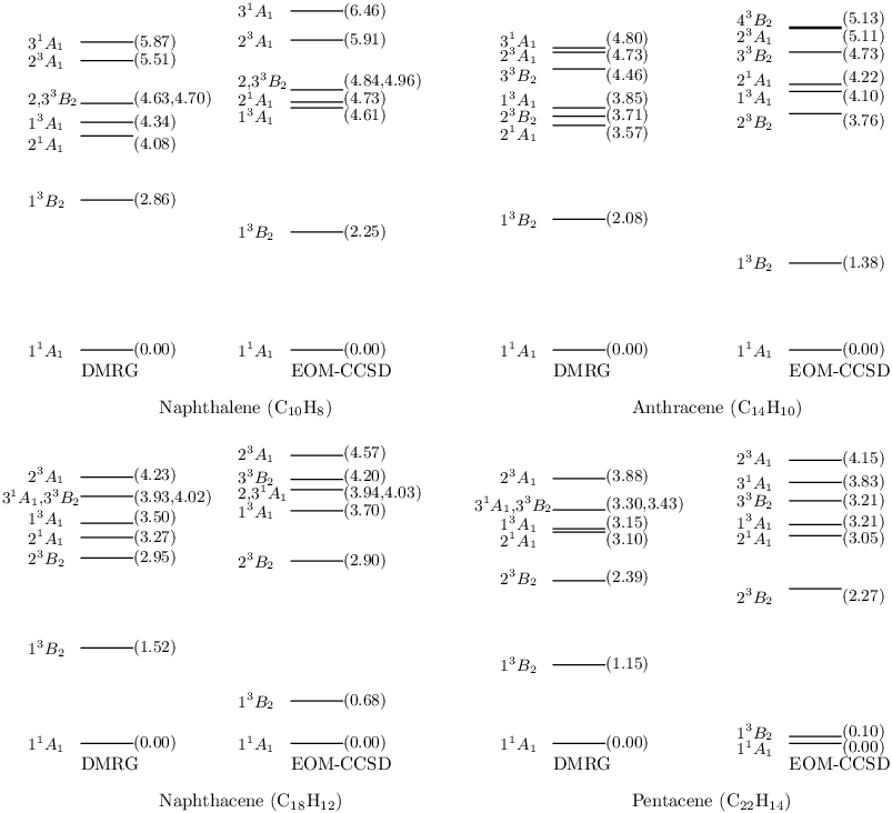
The ground state EOM-CCSD energies for the acenes are summarized in Table 1. We used our near-exact DMRG(500) excitation energies to examine the accuracy of the EOM-CC method in acenes. The EOM-CCSD and the DMRG symmetries and excitation energies are shown in Fig. 3. For the larger acenes, the EOM-CCSD excited states are in a qualitatively different order as compared to DMRG. Similarly, EOM-CCSD erroneously predicts a very small singlet-triplet gap for the longer acenes. This points to the necessity of including relatively high order correlation effects to accurately describe excitations in the acenes.
IV Conclusions
To overcome the computational and accuracy limitations of the traditional State-Averaged Davidson Algorithm, which requires both solving for and representing all states between the ground state and excited state of interest, we have investigated a number of new excited state algorithms within the context of the Density Matrix Renormalization Group (DMRG). In the Harmonic Davidson (HD) algorithm, using a shifted and inverted operator enabled us to directly solve for the excited state of interest. In the State-Averaged Harmonic Davidson (SA-HD) algorithm, we combined the HD method with an average over nearby excited states, to confer greater stability and overcome problems of root-flipping in the non-linear optimisation of the wavefunction.
To assess the accuracy, stability, and computational cost of these new methods we calculated the low-lying excited states in the acenes ranging from naphthalene to pentacene. We found that as expected, in addition to the size of the DMRG basis used, the accuracy was primarily determined by the number of states used in the state average. Thus the State-Averaged Davidson approach gave the least accuracy, the Harmonic Davidson algorithm, the highest, and the State-Averaged Harmonic Davidson lay in between depending on how many nearby states were included. The State-Averaged Harmonic Davidson algorithm converged smoothly without root-flipping so long as nearby “competing” states were included in the average.
We also argued that through the shift in the Harmonic Davidson algorithms we could piece together a complete excitation spectrum by targeting different regions with successively higher shifts. This we demonstrated by calculating some higher lying excited states in naphthalene.
Within the basis used, our DMRG excitation energies are near-exact and we have used them to assess the accuracy of the EOM-CCSD method in the acenes. We found that the EOM-CCSD excitation spectrum was qualitatively different from that of the DMRG for the larger acenes, which demonstrates the necessity of including higher-order correlations to properly describe the electronic spectrum of conjugated quasi-one-dimensional molecules.
Finally, we observe that the Harmonic Davidson algorithms studied here are quite general methods and are not limited to the Density Matrix Renormalisation Group. Thus they may be useful also to target excited states in other multi-reference theories, such as Complete Active Space Self-Consistent-Field theory.
Acknowledgements.
JH is funded by a Kekulé Fellowship of the Fond der Chemischen Industrie (Fund of the German Chemical Industry). GKC acknowledges support from Cornell University, Cornell Center for Materials Research, the David and Lucile Packard Foundation in Science and Engineering, and the National Science Foundation CAREER program CHE-0645380.References
- Yaron et al. (1998) D. Yaron, E. E. Moore, Z. Shuai, and J. Brédas, J. Chem. Phys. 108, 7451 (1998).
- White and Martin (1999) S. R. White and R. L. Martin, J. Chem. Phys. 110, 4127 (1999).
- Legeza et al. (2003a) Ö. Legeza, J. Röder, and B. A. Hess, Phys. Rev. B 67, 125114 (2003a).
- Fano et al. (1998) G. Fano, F. Ortolani, and L. Ziosi, J. Chem. Phys. 108, 9246 (1998).
- Shuai et al. (1997) Z. Shuai, J. L. Brédas, S. K. Pati, and S. Ramasesha, Proc. of SPIE 3145, 293 (1997).
- Chan and Head-Gordon (2002) G. K.-L. Chan and M. Head-Gordon, J. Chem. Phys. 116, 4462 (2002).
- Hallberg (2006) K. Hallberg, Advances in Physics 55, 477 (2006).
- Legeza et al. (2003b) Ö. Legeza, J. Röder, and B. A. Hess, Mol. Phys. 101, 2019 (2003b).
- Moritz et al. (2005) G. Moritz, A. Wolf, and M. Reiher, J. Chem. Phys. 123, 184105 (2005).
- Chan et al. (2004) G. K.-L. Chan, M. Kállay, and J. Gauss, J. Chem. Phys. 121, 6110 (2004).
- Hachmann et al. (2006) J. Hachmann, W. Cardoen, and G. K.-L. Chan, J. Chem. Phys. 125, 144101 (2006).
- Hachmann et al. (2007) J. Hachmann, J. Dorando, M. Avilés, and G. K.-L. Chan, J. Chem. Phys. (2007), submitted.
- Roos (1987) B. O. Roos, Adv. Chem. Phys. 69, 399 (1987).
- Schollwöck (2005) U. Schollwöck, Rev. Mod. Phys. 77, 259 (2005).
- Hallberg (2003) K. Hallberg, in Theoretical Methods for Strongly Correlated Electrons, edited by D. Senechal, A.-M. Tremblay, and C. Bourbonnais (Springer, New York, 2003), CRM Series in Mathematical Physics.
- Docken and Hinze (1972) K. K. Docken and J. Hinze, J. Chem. Phys. 57, 4928 (1972).
- Khait et al. (1995) Y. G. Khait, A. I. Panin, and A. S. Averyanov, Int. J. Quantum Chem. 54, 329 (1995).
- Knowles and Werner (1992) P. J. Knowles and H. J. Werner, Theor. Chim. Acta 4, 95 (1992).
- Hoffmann et al. (2002) M. R. Hoffmann, C. D. Sherill, M. L. Leininger, and H. F. Schaefer, Chem. Phys. Lett. 355, 183 (2002).
- Cancès et al. (2006) E. Cancès, H. Galicher, and M. Lewin, J. Comp. Phys. 212, 73 (2006).
- Morgan (1991) R. B. Morgan, Lin. Alg. Appl. 154-156, 289 (1991).
- Bai et al. (2000) Z. Bai, J. Demmel, J. Dongarra, A. Ruhe, and H. van der Vorst, Templates for the solution of algebraic eigenvalue problems: a practical guide (SIAM, Philadelphia, PA, 2000).
- Sleijpen and van der Vorst (1996) G. L. G. Sleijpen and H. A. van der Vorst, SIAM J. Matrix Anal. Appl. 17, 401 (1996).
- Tackett and Ventra (2002) A. Tackett and M. D. Ventra, Phys. Rev. B 66, 245104 (2002).
- Chan (2004) G. K.-L. Chan, J. Chem. Phys. 120, 3172 (2004).
- Crouzeix et al. (1994) M. Crouzeix, B. Philippe, and M. Sadkane, J. Sci. Comput. 15, 62 (1994).
- Saad (1993) Y. Saad, Numerical Methods for Large Eigenvalue Problems (Manchester University Press, Manchester, U.K., 1993).
- Davidson (1975) E. R. Davidson, J. Comput. Phys. 17, 87 (1975).
- Olsen et al. (1990) J. Olsen, P. Jørgensen, and J. Simons, Chem. Phys. Lett. 169, 463 (1990).
- Hehre et al. (1969) W. Hehre, R. Stewart, and J. Pople, J. Chem. Phys. 51, 2657 (1969).
- (31) T. D. Crawford, C. D. Sherrill, J. T. F. E. F. Valeev, R. A. King, M. L. Leininger, S. T. Brown, C. L. Janssen, E. T. Seidl, J. P. Kenny, and W. D. Allen, Psi 3.2 (2003), see www.psicode.org.
- Mitrushenkov et al. (2003) A. O. Mitrushenkov, R. Linguerri, P. Palmieri, and G. Fano, J. Chem. Phys. 119, 4148 (2003).
- Bartlett and Musiał (2007) R. J. Bartlett and M. Musiał, Rev. Mod. Phys. 79, 291 (2007).
- (34) C. Angeli, K. L. Bak, V. Bakken, O. Christiansen, R. Cimiraglia, S. Coriani, P. Dahle, E. K. Dalskov, T. Enevoldsen, B. Fernandez, et al., Dalton, a molecular electronic structure program, release 2.0 (2005), see www.kjemi.uio.no/software/dalton/.
- Kadantsev et al. (2006) E. S. Kadantsev, M. J. Stott, and A. Rubio, J. Chem. Phys. 124, 134901 (2006).
- Heinze et al. (2000) H. H. Heinze, A. Görling, and N. Rösch, J. Chem. Phys. 113, 2088 (2000).
- Nakatsuji et al. (1987) H. Nakatsuji, M. Komori, and O. Kitao, Chem. Phys. Lett. 142, 446 (1987).
- Kawashima et al. (1999) Y. Kawashima, T. Hashimoto, H. Nakano, and K. Hirao, Theor. Chim. Acta 102, 49 (1999).
- Hashimoto et al. (1996) T. Hashimoto, H. Nakano, and K. Hirao, J. Chem. Phys. 104, 6244 (1996).