Fermion masses, Leptogenesis and Supersymmetric SO(10) UnificationPreprint: IFIC/07-37
Abstract
Current neutrino oscillation data indicate the existence of two large lepton mixing angles, while Kobayashi-Maskawa matrix elements are all small. Here we show how supersymmetric SO(10) with extra chiral singlets can easily reconcile large lepton mixing angles with small quark mixing angles within the framework of the successful Fritzsch ansatz. Moreover we show how this is fully consistent with the thermal leptogenesis scenario, avoiding the so-called gravitino problem. A sizeable asymmetry can be generated at scales as low as possible within the leptogenesis mechanism. We present our results in terms of the leptonic CP violation parameter that characterizes neutrino oscillations.
pacs
12.10.Dm, 12.60.Jv, 14.60.St, 98.80.CqI Introduction
An endemic difficulty in unified gauge models is the understanding of fermion masses. Thanks to the brilliant series of experiments which led to the discovery of neutrino oscillations over the past ten years or so, we now have an improved knowledge of neutrino masses and mixings Maltoni:2004ei. The maximal atmospheric mixing angle and the large solar mixing angle both came as a surprise, at odds with naive unification–based expectations that lepton and quark mixings are similar. Indeed, although not mandatory, within unification models a similar structure for quark and lepton mixing is far easier to account for than what is currently established by observation. Several approaches have been considered in the literature to circumvent this problem, involving various types of extensions of the multiplet content Babu:1998wi; bertolini2004fms; Dermisek:2005ij; Altarelli:2004za; Nasri:2004rm.
A virtue of seesaw models is that they bring the possibility of decoupling the angles in the quark and lepton sectors by having additional Majorana-type terms for the latter schechter:1980gr. Moreover, seesaw models may account for the observed cosmological baryon excess through the elegant mechanism called leptogenesis Fukugita:1986hr. However in minimal supergravity models, with 100 GeV to 10 TeV the supersymmetric type-I seesaw scenario leads to an overproduction of gravitinos after inflation Khlopov:1984pf; Ellis:1984eq unless the reheat temperature is restricted to be much lower than that required for successful leptogenesis Kawasaki:2004qu. One possible way out is resonant leptogenesis Pilaftsis:2005rv as indeed suggested in Ref. Akhmedov:2003dg. Another alternative has been considered in Ref. Farzan:2005ez requires going beyond the minimal seesaw by adding a small R-parity violating term in the superpotential.
Here we consider an alternative approach to supersymmetric SO(10) unification that involves mainly an extension of the lepton sector and a novel realization of the seesaw mechanism already discussed previously Hirsch:2006ft; Malinsky:2005bi. We show how the observed structure of lepton masses and mixings fits together, thanks to the presence of the extra states, with the requirements of a predictive pattern of quark mixing, encoded within the successful Fritzsch ansatz Fritzsch:1977vd. Moreover, we show explicitly how such extended supersymmetric SO(10) seesaw scheme provides a realistic scenario for thermal leptogenesis, avoiding the so-called gravitino problem. Our approach is phenomenological in sipirit. Hence we do not seek to derive a full-fledged unified theory of flavour incorporating a specific symmetry, such as babu:2002dz; Altarelli:2005yx; Hirsch:2006je; Hirsch:2005mc; Hirsch:2007kh to the unified gauge group level.
The paper is organized as follows. In Sec. II we discuss the limitations of minimal supersymmetric type-I seesaw in naturally providing a framework for thermal leptogenesis in agreement with bounds on the reheat temperature after inflation, in Sec. III we recall the basic features of the considered model, while ansatzes for the coupling matrices are discussed in Sec. IV. In Sec. V we discuss the calculation of the final baryon number asymmetry from the decay asymmetry of the lightest singlet. There we discuss how we can use results obtained previously on production and washout factors in the seesaw type-I case also in our extended seesaw model. We show that leptogenesis scenario is consistent both with the reheat temperature constraint as well as with fitting the lepton and quark mixing angles within the successful Fritzsch ansatz.
II Minimal supersymmetric seesaw leptogenesis
In the most general seesaw model the Dirac fermion mass terms arise from the couplings of the 16 with the 10 and 126, while the diagonal entries in the seesaw neutrino mass matrix arise only from the couplings of the 16 with the 126. The mass matrix expressed in the basis is , is given as Valle:2006vb,
| (1) |
where the 16 denotes each chiral matter generation while the 10 and 126 are Higgs-type chiral multiplets. Here , and denote the Yukawa couplings of the 10 and 126, respectively. These are all symmetric in flavour, the symmetry of results from the Pauli principle, while that of follows from SO(10).
Minimization of the Higgs scalar potential leads to a vev seesaw relation
| (2) |
consistent with the desired vev hierarchy , where is the standard vev and are the vacuum expectation values (vevs) giving rise to the Majorana terms.
Before we display our proposed model it is useful to consider the case of the Minimal type-I seesaw Minkowski:1977sc. This consists in taking in the above equations. Although not generally consistent with SO(10) in the presence of the 126, this approximation is suitable for our purposes as the extension we will be discussing is tripletless, the 126 being replaced by 16’s.
The matrix is diagonalized by performing a a unitary transformation ,
| (3) |
whose form is given explicitly as a perturbation series in Ref. schechter:1982cv. The effective mass matrix of the three light neutrinos is given as
| (4) |
The smallness of light neutrino masses follows dynamically from Eq. (4), since is large.
In order to reproduce the observed pattern of quark masses and CP violation we assume the complex matrix to have the form
| (5) |
with complex and real. Notice that the large observed lepton mixing angles can always be reconciled with the small quark mixing angles thanks to the presence of the coupling matrices which exist only for neutrinos (in the limit of unbroken D-parity one has ). However, in a unified theory where a flavour symmetry is assumed to predict the lepton mixing angles, it becomes a real challenge to account naturally also for the quark mixing angles.
Now we turn to cosmology. One of the attractive features of seesaw models is that they open the possibility of accounting for the observed cosmological matter-antimatter asymmetry in the Universe through the leptogenesis mechanism Fukugita:1986hr. This requires the out-of-equilibrium decays of the heavy “right-handed” neutrinos (see Fig. 1) to take place before the electroweak phase transition, and the presence of CP violation in the lepton sector. The tree level and one loop diagrams for decay that interfere in order to generate a lepton asymmetry of the universe are shown.

These decays generate the asymmetry,
| (6) |
Here we recall the estimate of such asymmetry, as given in Ref.covi:1996wh. The relevant amplitudes follow from the initial Lagrangian
| (7) |
Here it is sufficient just to sketch their structure. At the tree level we have
| (8) |
while for the one-loop it is only necessary to evaluate the vertex contribution,
| (9) |
where is some complex loop function. Now tree level plus one loop will be proportional to
| (10) |
so that the asymmetry is
| (11) |
Now using Eq. (8) and Eq. (9) we can write
| (12) |
Finally we get, in the case of hierarchical right-handed neutrinos,
| (13) |
Note that in this limit the contribution of the self energy has the same dependence on the couplings and is already included. The lepton (or B-L) asymmetry thus produced then gets converted, through sphaleron processes, into the baryon asymmetry Fukugita:1986hr, observed to be . In order to provide an acceptable framework for leptogenesis, and taking into account the presence of washout effects, the asymmetry we need is or larger, for the same values of parameters that reproduce the observed small neutrino masses, Eq. (4). In order to generate this asymmetry thermally one requires the Universe to reheat after inflation to a very high temperature Buchmuller:2004nz; Davidson:2002qv; Hamaguchi:2001gw; Barbieri:1999ma
| (14) |
Such large scale leads to an overproduction of cosmological gravitinos. In minimal supergravity models, with 100 GeV to 10 TeV gravitinos are not stable, decaying during or after Big Bang Nucleosynthesis (BBN). Their rate of production can be so large that subsequent gravitino decays completely change the standard BBN scenario. Since the abundance of gravitinos is proportional to such “gravitino crisis” can only be prevented by requiring a low enough reheat temperature after inflation Khlopov:1984pf; Ellis:1984eq. A recent detailed analysis gives a stringent upper bound
| (15) |
when the gravitino has hadronic decay modes Kawasaki:2004qu. Therefore, thermal leptogenesis seems difficult to reconcile with low energy supersymmetry if gravitino masses lie in the range suggested by the simplest minimal supergravity models. One possible way out is to have resonant leptogenesis Pilaftsis:2005rv as suggested in Ref. Akhmedov:2003dg. Another alternative considered in Ref. Farzan:2005ez requires going beyond the minimal seesaw by adding a small R-parity violating term in the superpotential. In the following we discuss quantitatively the alternative suggestion made in Hirsch:2006ft in the context of the extended supersymmetric seesaw scheme.
III The new extended seesaw model
For definiteness we work in the context of the supersymmetric SO(10) unified model considered in Ref.Malinsky:2005bi; Hirsch:2006ft. The gauge symmetry and D-parity are broken by 45 and 210 multiplets at the unification scale. The B-L symmetry breaks at lower scale thanks to expectation values of the fields in the 16, instead of the more familiar left and right triplets present in 126 which lead to the standard seesaw mechanism. Gauge couplings unification can not fix the B-L breaking scale, which can be relatively low, as shown in Ref. Malinsky:2005bi. The possibility of a low B-L breaking scale also fits with the observed neutrino masses. The relevant Yukawa couplings leading to neutrino masses are
| (16) |
Note that a direct Majorana mass term for the singlet fields is forbidden by an additional imposed symmetry and the fact that the only singlet scalar present () is odd under D-parity, while are even under D-parity. For the same reason, cannot couple to , but a bare mass is allowed Hirsch:2006ft. As we will show leptogenesis allows this mass to be of the order of TeV. We also introduce a soft term breaking , which allows mixing between the scalar components of these fields ,
| (17) |
This will then give a neutrino mass matrix, in the basis (, , , ):
| (18) |
where, , and are the vevs for the fields , and respectively and is the breaking entry. Besides the three light neutrinos, this mass matrix will give two heavy states which are dominantly the right-handed neutrino and the singlets , and a lighter state . Notice that we will not impose any specific family symmetry. In Sec. IV.2 we will, however, consider the case where the are restricted to follow the Fritzsch texture for the quark sector.
III.1 Light neutrinos
Using the seesaw diagonalization prescription given in Ref. schechter:1982cv we obtain the effective left-handed light neutrino mass matrix as Hirsch:2006ft,
| (19) |
where . Since the parity breaking scale is much higher than the scale at which the left-right symmetry breaks, and this in turn is higher than the electroweak symmetry breaking scale, one has the “vev-seesaw” relation
| (20) |
where is determined by the SO(10) breaking vevs. In the following we will take this proportionality constant equal to one and therefore write Eq. (19) as
| (21) |
Note that the neutrino masses are suppressed by the unification scale instead of the B-L scale. As noted in Malinsky:2005bi we need two pairs of 16 in order to boost up the neutrino mass scale and bring in an independent flavour structure beyond that of the charged Dirac couplings, constrained by the quark sector phenomenology.
Now we want to extract as much information from the low energy neutrino data as possible. The matrix can be diagonalized as,
| (22) |
where we use the standard parameterization from Ref.schechter:1980gr and now adopted by the PDG
| (23) |
The values of and are known to some degree from experiment and we want to turn this information into the parameters of the theory, defined by Eq. (16). Of course we have too little experimental information, three angles and two mass differences, to be able to reconstruct in full the three matrices and the vector .
III.2 Heavy neutrinos
Let us now turn to the discussion of the heavy neutrinos. The following terms in the Lagrangian,
| (24) | |||||
lead to a mass matrix in the basis (, , ):
| (25) |
which determines the masses of the heavy neutrinos. Now in order to get the states with physical masses we diagonalize this mass matrix in three steps. We start by diagonalizing the matrix . We define
| (26) |
where and are unitary matrices. Then we define new fields
| (27) |
so that in the basis we have
| (28) |
with
| (29) |
and
| (30) |
Now we rotate the fields and to obtain the almost degenerate states . This is done by defining a new matrix
| (31) |
that obeys
| (32) |
with , and
| (33) |
We now have to perform the final rotation in order to get the physical states for these heavy neutrinos. As we have seen in the discussion of the light neutrinos, the amount of -violation must be small, therefore Eq. (33) can be approximately diagonalized using the techniques of Ref.schechter:1982cv. We obtain
| (34) |
with , where
| (35) |
and
| (36) |
If we assume that the eigenvalues of are hierarchical we get also a hierarchical spectrum for the heavy states, , namely, . In order to evaluate the asymmetry generated we must evaluate the couplings of the mass eigenstates. For this we notice that
| (37) |
and a simple calculation gives
| (38) |
which allows us to write
| (39) | |||||
where we have used
| (40) |
With this we can rewrite the relevant part of the Lagrangian of Eq. (16) in terms of the eigenstates (we drop the primes from now on),
| (41) |
where
| (42) |
where denotes the projection of the relevant light MSSM Higgs doublet into the directions of the defining Higgs doublets living in , and are the projections of the light MSSM-like Higgs doublet onto the defining Higgs doublets in the and is the mass of the .
III.3 Calculation of the Asymmetry


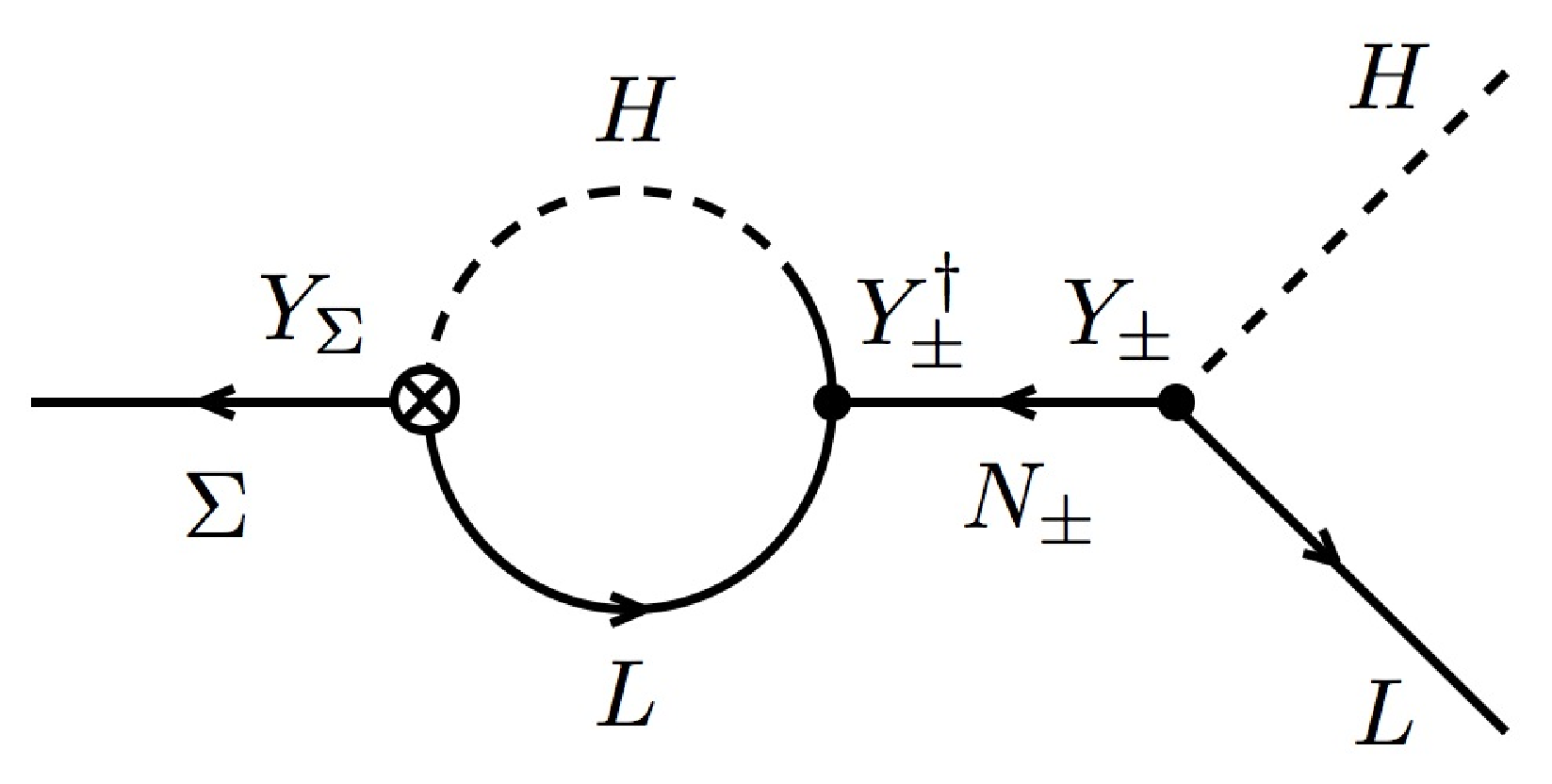
We now discuss the issue of leptogenesis in this model. It can occur only after the local SO(10) symmetry is broken. This will take place through the out-of-equilibrium decay of the singlet fermion . The total width of is given by (treating as a column vector)
| (43) |
where is given in Eq. (42).
The asymmetry coming from the diagrams of Fig. 2 involves the sum over which reduces to the sum over the lightest pair of the (almost degenerate) states with masses . A comparison of the diagrams in Fig. 2 and Fig. 1 gives the following dictionary
| (44) |
We have then for the numerator
| (45) | |||||
where we have defined: . Comparing with Eq. (42) we get
| (46) |
Putting everything together we finally obtain
| (47) |
It is important to note that, in contrast to the asymmetry in the minimal seesaw discussed in the previous section, is not constrained by the light neutrino masses. This can essentially be understood by the fact that the neutrino mass, see eq.(19) and eq.(20), is suppressed by the small ratio , whereas in the calculation of , the small quantity appears quadratically in the numerator and the denominator, and thus cancels. can therefore be much larger than in the minimal seesaw case, independent of the light neutrino masses. Consequently, there is also no lower bound on from the asymmetry parameter .
IV Ansatzes for the Coupling Matrices
We now estimate the resulting CP asymmetry needed for leptogenesis making use of the current values of the neutrino oscillsation parameters given in Maltoni:2004ei. A simple ansatz is to assume that it comes just from the Dirac phase of the three-neutrino lepton mixing matrix assuming the unitary approximation. In this approximation the asymmetry is proportional to the unique CP invariant parameter that can be probed in neutrino oscillations. The maximum value of the asymmetry that can be achieved is obtained by varying randomly all the other model parameters and the results are displayed at each point of the plane (,).
IV.1 Generic case: non-hierarchical
We start by considering a non-hierarchical ansatz for the coupling matrices. In order to reduce the unknowns we assume that both and matrices are proportional to the standard SO(10) Dirac Yukawa coupling matrix , which is symmetric, namely
| (48) |
With this choice Eq. (21) can be written as,
| (49) |
where
| (50) |
Clearly, the projective nature of will not explain the neutrino data, therefore we need the contribution of . The atmospheric scale can easily be reproduced with , and , for .
With the assumptions of Eq. (48) we can solve for the Yukawa matrix in terms of the experimentally observed neutrino oscillation parameters via
| (51) |
which also involves other parameters of the model.
With this ansatz and the choice we take the lepton mixing parameters in the range allowed by the experiment. At the latest neutrino oscillation data give Maltoni:2004ei
| (52) |
In addition we take the other model parameters in the following ranges,
| (53) |
With these values we can see the resulting , and values that follow from our ansatz in Fig. 3. They show that it is possible to fit the neutrino data with this simple type of ansatz. The resulting CP asymmetry produced is given in Fig. 4. Here we have calculated the maximum value of the asymmetry that can be achieved at each point of the (,) plane, varying randomly all the other parameters. Clearly the sizeable values of the asymmetry can be obtained, especially for large and , as expected, so that the necessary CP asymmetry needed for leptogenesis can be achieved.

.

One sees that large values of the asymmetry, compatible with the experimental data, can be achieved in the full parameter space, even for very small and values. However the ansatz is manifestly inconsistent with the successful Fritzsch texture for the quark masses.
IV.2 Fritzsch case: hierarchical
It is natural to ask whether our SO(10) model described by the Lagrangian of Eq. (16) can provide thermal leptogenesis while reconciling the successful Fritzsch texture for the quark masses with the observed structure of lepton masses and mixings that follow from neutrino oscillation experiments. To this end we now assume that the Yukawa’s involved in neutrino mass generation are also restricted by the Fritzsch ansatz for the quark couplings, given in Eq. (5), with complex and real. Aware of the fact that the phases will be necessary in computing the final asymmetry, we will, for the moment take the ansatz parameters all real, as
| (54) |
These values imply a strong hierarchy among the Yukawa couplings. With this choice, let us now look at the neutrino mass matrix. It is clear from Eq. (21) that this hierarchy must be corrected by a suitable hierarchy in the coupling matrix. In fact Eq. (21) can be “solved” for as
| (55) |
where is obtained from
| (56) |
where , being, in general, an arbitrary non-symmetric matrix. Now is expressed as a combination of neutrino data and additional parameters, for which we take random values.
We have performed a random study of this Fritzsch ansatz assuming as our ansatz that with and taking random values of order one in various ways. We have found that in this case, for example for in the range GeV, of few TeV and GeV one indeed obtains a viable solution. One finds that some of the entries of are small (of order ) in order to compensate for the corresponding smallness of in Eq. (5).
We have also explicitly calculated the value of the asymmetry for this ansatz as explained above. The results are shown in Fig. 5 for the case of the hierarchical ansatz with the current neutrino oscillation parameters from Maltoni:2004ei and the Dirac phase is .


One sees that, in this case, values of the asymmetry of order - can only be obtained for large values of and . Therefore, this scenario can be potentially probed by the future neutrino oscillation measurements.
Larger values of the CP asymmetry compatible with current neutrino oscillation measurements can be found for other ansatze of the current model using the Fritzsch texture. For instance, if we consider with symmetric, or diagonal and , one can obtain very large values of the asymmetry even for very small values of and , as illustrated in Fig. 6.


V Asymmetry washout, singlet production and the sphaleron constraint
Generating a large enough asymmetry in the decay of the lightest singlet is a necessary, but not a sufficient condition for successful leptogenesis. Additional conditions are required, before one can conclude that any given model can generate the required baryon asymmetry.
The first condition to be satisfied is the out-of-equilibrium decay of the heavy singlet, which is nothing but the basic Sakharov condition Sakharov:1967dj. This requires that the decay rate is smaller than the expansion rate of the universe, i.e. at the decay epoch. For large , say, of order of the expansion rate, part of the asymmetry produced in the decays will be washed out by inverse scattering processes violating lepton number. This constraint will thus put an upper limit on the couplings of to the leptons (and Higgses) for any given mass . Second, we need to produce a sufficient number of singlets in the early universe. Singlets could be either produced by their couplings to the thermal bath or through the decay of some heavier particle, which was present in the universe at earlier times. Obviously, a sufficiently strong direct thermal production requires a minimum value for the couplings of , whereas the second option does not. The third constraint comes from the fact that the decays have to take place at a time early enough that the SM sphalerons are still in equilibrium, otherwise we will produce a lepton number, but no non-zero baryon number. This constraint puts a lower limit on , , independent of the production mechanism of .
To accurately calculate the first two of the above conditions, in principle, one needs to set up a network of Boltzmann equations, which in general can only be solved numerically Kolb:1990vq. However, under certain simplifying assumptions, one can derive approximate analytical solutions which reproduce the full, numerical calculations quite well. Several analytical approximations have been proposed in the literature, see for example Kolb:1990vq; Nielsen:2001fy; Buchmuller:2002rq. In our earlier paper Hirsch:2006ft we have used the following approximate form for the washout factor:
| (57) |
where , with being the expansion rate of the universe Kolb:1990vq. Ref. Buchmuller:2002rq has numerically solved the Boltzmann system for the case of the simpler type-I seesaw. In this case the decay width of the lightest right-handed neutrino is proportional to , and the authors of Buchmuller:2002rq define the “effective mass” parameter , where is the mass of the lightest right-handed neutrino and the SM vev. Thermal equilibrium for the right-handed neutrino is reached for an “equilibrium mass” eV, for which by definition . The full numerical calculation is then very well approximated by
| (58) |
with
| (59) |
and the numerical values
| (60) |
We can make use of the results of Buchmuller:2002rq with the straightforward replacement,
| (61) |
Our more complicated setup of Boltzmann equations then is solved approximately by the fit eq. (58). Note, that this implicitly assumes 11 1 The same assumption is used in the fit leading to this equation in the simpler type-I seesaw that the heavier singlets are sufficiently decoupled so as to not contribute significantly to the washout.
As seen in Fig. (7) eq. (58) and eq. (57) lead to very similar results for , The two forms differ, however, for . This can be traced to the fact that eq. (58) also accounts for the suppressed production in the weak coupling regime, while eq. (57) does not. For definiteness, in the plots shown below, we have used eq. (58).

We have also used the constraint imposed by the condition that the decay of the singlets must happen while the sphalerons are still active. We estimate the sphaleron time using
| (62) |
with denoting the energy at which the electro-weak phase transition occurs, the effective number of degrees of freedom and the reduced Planck mass. We cut all points with . This is, of course, a rough approximation to the real, dynamical situation. However, we believe it to be sufficiently accurate for deriving order of magnitude constraints on the model parameters. Finally, when converting the produced lepton asymmetry to the baryon asymmetry, we have to take into account an efficiency factor for the sphalerons. This factor has been calculated in Khlebnikov:1988sr to be
| (63) |
where () is the number of families (Higgses). Numerically this factor is .
Fig. (8) shows as an example the resulting as a function of for a numerical scan using the ansatz shown in fig.(5), to the left. The light/dark (green/red) area is the calculated range for without/with the sphaleron constraint. One sees that the different constraints discussed above conspire to choose a rather well-defined allowed range for the parameter in this case. A large enough baryon asymmetry can be obtained roughly for GeV, for the range of the other parameters as given in eq. (53). It is amusing to note, that the requirement of producing a sufficient number of singlets and the sphaleron constraint lead to rather similar lower cuts on 22 2 The same will occur for the seesaw type-I: The sphaleron constraints provides a lower cut on the “effective mass parameter” ..

We have repeated this exercise for all the different ansätze discussed above. The resulting allowed ranges for the parameters and are shown in fig. (9). As shown in this figure, the random non-hierarchical ansatz and the hierarchical ansatz shown in the right panel of Fig. 6 lead to the widest allowed ranges for and .

| [GeV] | [GeV] | [GeV] | [GeV] | [GeV] | [] |
|---|---|---|---|---|---|
| Non-hierarchical | |||||
| 8.3 | 1.2 | 4.1 | 5.0 | 2.6 | 6.3 |
| 9.8 | 2.3 | 9.3 | 1.2 | 6.1 | 5.0 |
| Hierarchical 5a | |||||
| 3.5 | 1.2 | 3.6 | 6.2 | 6.7 | 4.9 |
| 2.9 | 1.1 | 4.6 | 6.8 | 5.7 | 5.8 |
| Hierarchical 5b | |||||
| 1.8 | 6.6 | 2.1 | 6.4 | 3.8 | 5.2 |
| 8.3 | 2.5 | 6.1 | 6.2 | 9.8 | 4.8 |
| Hierarchical 6a | |||||
| 2.9 | 2.9 | 1.6 | 3.6 | 6.0 | 5.1 |
| 3.3 | 8.3 | 2.5 | 1.3 | 1.4 | 5.8 |
| Hierarchical 6b | |||||
| 1.0 | 1.8 | 1.9 | 1.1 | 2.0 | 5.4 |
| 3.4 | 2.8 | 1.5 | 1.5 | 2.5 | 5.9 |
Before we close this section let us briefly illustrate possible values for the relevant parameters. These are , the masses of the three iso-singlet neutrinos and the resulting baryon asymmetry . Some examples are given in table 1 for each of the scenarios we have discussed. As one can see the acceptable baryon asymmetry may arise for rather low scales, in contrast to the (simpler) seesaw type-I schemes. Note, however that the values given in the table are by no means unique, and are also not meant to be “representative” of the classes. The generation of the baryon asymmetry is far easier in this context than in the traditionl seesaw model. The presence of the new singlets allows us to have, in addition, acceptable textures for the quark and lepton mixing angles.
VI Conclusions
We have reviewed the argument that in minimal type-I SO(10) seesaw one can not easily reconcile the thermal leptogenesis scenario with the successful Fritzsch texture for the quarks and an acceptable pattern of lepton masses and mixings that follow from neutrino oscillation experiments. This is due to the fact that the large seesaw scale needed to account for small neutrino masses leads to an overproduction of cosmological gravitinos, which destroys the standard predictions of Big Bang Nucleosynthesis (BBN). Barring the very special case of resonant leptogenesis, one must go beyond the minimal type-I seesaw mechanism.
In this paper we have studied in some detail an extended seesaw scenario as a natural way to overcome this limitation. The proposed extension has the added virtue of providing a natural setting for reconciling the observed structure of neutrino mixing angles with the strong hierarchy among quark masses and the smallness of the quark mixings. While this can always be accommodated in a “generic” unified theory with arbitrary multiplet content, it becomes a real challenge for unified predictive models of flavour.
We have provided a quantitative study of fermion masses and (an approximative calculation of) leptogenesis in the context of supersymmetric SO(10) Unification. Our approach was phenomenological in that we have not assumed a specific flavour symmetry. We have shown how thermal leptogenesis can occur at relatively low scale through the decay of a new singlet, thereby avoiding the gravitino crisis. Washout of the asymmetry is effectively suppressed by the absence of direct couplings of the singlet to leptons. For illustration we have shown how one can accommodate current oscillation neutrino data and the required value for the asymmetry for successful leptogenesis even if the only source of CP violation is the Dirac phase in the low energy neutrino mixing matrix. Finally, we note that we have not taken into account flavour effects Abada:2006ea; Nardi:2006fx in the calculation of the asymmetry. However, we believe that the absence of a lower bound on in our model is independent on whether flavour effects are taken into account or not.
Using the Fritzsch texture we have found that some ansatze lead to acceptable values of the asymmetry of order - only for large values of and . Therefore, these scenarios can be potentially probed by the future neutrino oscillation measurements, as the required value of the CP invariant is nearly maximal. In contrast, we have also presented alternative Fritzsch-type ansatze leading to substantially larger values of the CP asymmetry, even for very small values of and . We have also discussed, how to approximately treat the conversion of the decay asymmetry to the baryon asymmetry, without resorting to a full numerical solution of the Boltzmann equations. To this end, we made use of some approximation formulas derived previously for seesaw type-I and discussed how they can be adapted to cover also our more complicated case.
In summary, our extended seesaw scenario provides a way of reconciling the lepton and quark mixing angles with thernal leptogenesis in a unified scenario. While this by itself does not constitute a complete theory of fermion masses and leptogenesis, at least it provides a useful first step towards an ultimate unified theory incorporating flavour.
Acknowledgments
Work supported by MEC grants FPA2005-01269 and FPA2005-25348-E, by Generalitat Valenciana ACOMP06/154, by European Commission Contracts MRTN-CT-2004-503369 and ILIAS/N6 WP1 RII3-CT-2004-506222.
References
- (1) For an updated review see M. Maltoni, T. Schwetz, M. A. Tortola, and J. W. F. Valle, New J. Phys. 6, 122 (2004), hep-ph/0405172 (v6) provides updated results as of September 2007; previous works by other groups are referenced therein and in Fogli:2005cq.
- (2) G. L. Fogli, E. Lisi, A. Marrone and A. Palazzo, Prog. Part. Nucl. Phys. 57 (2006) 742 [hep-ph/0506083].
- (3) K. S. Babu, J. C. Pati, and F. Wilczek, Nucl. Phys. B566, 33 (2000), hep-ph/9812538.
- (4) S. Bertolini, M. Frigerio, and M. Malinský, Physical Review D 70, 095002 (2004).
- (5) R. Dermisek and S. Raby, Phys. Lett. B622, 327 (2005), hep-ph/0507045.
- (6) G. Altarelli and F. Feruglio, New J. Phys. 6, 106 (2004), hep-ph/0405048.
- (7) S. Nasri, J. Schechter, and S. Moussa, Phys. Rev. D70, 053005 (2004), hep-ph/0402176.
- (8) J. Schechter and J. W. F. Valle, Phys. Rev. D22, 2227 (1980).
- (9) M. Fukugita and T. Yanagida, Phys. Lett. B174, 45 (1986).
- (10) M. Y. Khlopov and A. D. Linde, Phys. Lett. B138, 265 (1984).
- (11) J. R. Ellis, J. E. Kim, and D. V. Nanopoulos, Phys. Lett. B145, 181 (1984).
- (12) M. Kawasaki, K. Kohri, and T. Moroi, Phys. Rev. D71, 083502 (2005), astro-ph/0408426.
- (13) A. Pilaftsis and T. E. J. Underwood, Phys. Rev. D72, 113001 (2005), hep-ph/0506107.
- (14) E. K. Akhmedov, M. Frigerio, and A. Y. Smirnov, JHEP 09, 021 (2003), hep-ph/0305322.
- (15) Y. Farzan and J. W. F. Valle, Phys. Rev. Lett. 96, 011601 (2006), hep-ph/0509280.
- (16) M. Hirsch, J. W. F. Valle, M. Malinsky, J. C. Romao, and U. Sarkar, Phys. Rev. D75, 011701 (2007), hep-ph/0608006.
- (17) M. Malinsky, J. C. Romao, and J. W. F. Valle, Phys. Rev. Lett. 95, 161801 (2005), hep-ph/0506296.
- (18) H. Fritzsch, Phys. Lett. B73, 317 (1978).
- (19) K. S. Babu, E. Ma, and J. W. F. Valle, Phys. Lett. B552, 207 (2003), hep-ph/0206292.
- (20) G. Altarelli and F. Feruglio, Nucl. Phys. B741, 215 (2006), hep-ph/0512103.
- (21) M. Hirsch, E. Ma, J. C. Romao, J. W. F. Valle, and A. Villanova del Moral, Phys. Rev. D 75, 053006 (2007), hep-ph/0606082.
- (22) M. Hirsch, A. Villanova del Moral, J. W. F. Valle, and E. Ma, Phys. Rev. D72, 091301 (2005), hep-ph/0507148.
- (23) M. Hirsch, A. S. Joshipura, S. Kaneko, and J. W. F. Valle, Phys. Rev. Lett. 99, 151802 (2007), hep-ph/0703046.
- (24) For an updated seesaw review see J. W. F. Valle, J. Phys. Conf. Ser. 53, 473 (2006), hep-ph/0608101, Review based on lectures at the Corfu Summer Institute on Elementary Particle Physics in September 2005.
- (25) P. Minkowski, Phys. Lett. B67, 421 (1977).
- (26) J. Schechter and J. W. F. Valle, Phys. Rev. D25, 774 (1982).
- (27) L. Covi, E. Roulet, and F. Vissani, Phys. Lett. B384, 169 (1996), hep-ph/9605319.
- (28) W. Buchmuller, P. Di Bari, and M. Plumacher, Ann. Phys. 315, 305 (2005), hep-ph/0401240.
- (29) S. Davidson and A. Ibarra, Phys. Lett. B 535 (2002) 25 [arXiv:hep-ph/0202239].
- (30) K. Hamaguchi, H. Murayama and T. Yanagida, Phys. Rev. D 65 (2002) 043512 [arXiv:hep-ph/0109030].
- (31) R. Barbieri, P. Creminelli, A. Strumia and N. Tetradis, Nucl. Phys. B 575 (2000) 61 [arXiv:hep-ph/9911315].
- (32) A. D. Sakharov, Pisma Zh. Eksp. Teor. Fiz. 5 (1967) 32 [JETP Lett. 5 (1967 SOPUA,34,392-393.1991 UFNAA,161,61-64.1991) 24].
- (33) E. W. Kolb and M. S. Turner, Front. Phys. 69 (1990) 1.
- (34) H. B. Nielsen and Y. Takanishi, Phys. Lett. B 507 (2001) 241 [arXiv:hep-ph/0101307].
- (35) W. Buchmuller, P. Di Bari and M. Plumacher, Nucl. Phys. B 643 (2002) 367 [arXiv:hep-ph/0205349].
- (36) S. Y. Khlebnikov and M. E. Shaposhnikov, Nucl. Phys. B 308 (1988) 885.
- (37) W.-M. Yao et al., J. Phys. G 33, 1 (2006), Particle Data Group, http://pdg.lbl.gov/
- (38) A. Abada, S. Davidson, A. Ibarra, F. X. Josse-Michaux, M. Losada and A. Riotto, JHEP 0609, 010 (2006) [arXiv:hep-ph/0605281].
- (39) E. Nardi, Y. Nir, E. Roulet and J. Racker, JHEP 0601, 164 (2006) [arXiv:hep-ph/0601084].