A self-consistent first-principles calculation scheme for correlated electron systems This paper is to be published in J. Phys. Condens. Matter (2007).
Abstract
A self-consistent calculation scheme for correlated electron systems is created based on the density-functional theory (DFT). Our scheme is a multi-reference DFT (MR-DFT) calculation in which the electron charge density is reproduced by an auxiliary interacting Fermion system. A short-range Hubbard-type interaction is introduced by a rigorous manner with a residual term for the exchange-correlation energy. The Hubbard term is determined uniquely by referencing the density fluctuation at a selected localized orbital. This strategy to obtain an extension of the Kohn-Sham scheme provides a self-consistent electronic structure calculation for the materials design. Introducing an approximation for the residual exchange-correlation energy functional, we have the LDA+U energy functional. Practical self-consistent calculations are exemplified by simulations of Hydrogen systems, i.e. a molecule and a periodic one-dimensional array, which is a proof of existence of the interaction strength as a continuous function of the local fluctuation and structural parameters of the system.
1 Introduction
Inclusion of the short-range correlation effect (SRCE) is a long-term request for the first-principles electronic structure calculation based on the density functional theory (DFT).[1, 2] In principles, it is possible, since the strategy introduced by Hohenberg, Kohn and Sham was shown to be given by a rigorous variational principle.[3, 4, 5, 6] Although the method should give formally an exact calculation scheme for the Coulomb system, the energy density functional is not perfectly known at present. Plausible approximation schemes have been proposed and utilized.[2, 7, 8, 9] However, they have their own limitation. For example, the local-density approximation (LDA) is known to conclude a metallic ground state for the Mott insulator La2CuO4.[10, 11, 12, 13, 14, 15, 16] This failure of LDA is a central problem of DFT for which we hope inclusion of SRCE to be a solution. Especially, when LDA gives near degeneracy in the ground state, proper treatment of SRCE can lift the degeneracy to have the non-degenerated ground state implying formation of the Mott gap. This assumption may be widely accepted as a natural conclusion according to the study of the Hubbard models.[17, 18]
Here we should note that the Kohn-Sham scheme has flexibility and it can be adjusted even for the Mott insulator. If we introduce a wavefunction of an entangled state as the Kohn-Sham ground-state wavefunction, the excitation spectrum for the Kohn-Sham system may change. This implies that response of the system has changed. Considering the adiabatic shift of the ground state as a function of some outer parameters like the external electro-magnetic field, there should be an essential change as a consequence of the introduction of SRCE in the Kohn-Sham scheme. Even if we consider the density functional theory for the ground state of the Coulomb system, this extended scheme allows us to handle the correlated electron system by the density functional theory.
Thus we have yet many possible approaches for the practical computation as realization of the Kohn-Sham scheme in an extended formulation. Actually, the Kohn-Sham equation is regarded as an auxiliary equation to realize the optimization process of the single particle density . In this paper, we consider this physical quantity as a central order parameter of the electron system. Usually, a system of non-interacting Fermions is utilized to describe in the Kohn-Sham scheme. Interestingly, we are allowed to consider interacting Fermion systems, which can be used to replace the non-interacting Kohn-Sham system. This is called the multi-reference density functional theory (MR-DFT).[19, 20, 22, 23, 25] To develop direct description of a Mott insulating state, one of the authors defined a kind of MR-DFT.[26] Utilizing this formulation called the extended Kohn-Sham scheme (EKSS), one has a chance to detect Coulomb suppression of fluctuation, which is not found in .
The interacting Kohn-Sham system has been originally motivated in the hybrid approach with the configuration interaction (CI) scheme in the theory of the quantum chemistry.[19, 20, 21, 22, 23, 24, 25] In the hybrid density functional theory, people utilized 1) a full or a part of elements or integrals of the density matrix[22] or 2) restriction of the searching space[23] in the constrained minimization to define the energy density functional. Knowledge on the modified energy density functional, however, are not enough. A proof of existence of the minimum in the constrained search is demanded. On the contrary, it is possible to formulate MR-DFT in another way by referring the original Levy-Lieb energy functional.[26, 27]
In this paper, focusing on the fluctuation reference method,[27] we will discuss a self-consistent calculation scheme of MR-DFT. The method is shown to be a kind of the renormalization method to find a fixed effective interacting Hamiltonian. A practical approximation for the residual exchange-correlation energy functional allows us to confirm that the scheme do give the self-consistent solution. We will give a report on the first application of our scheme in two types of the Hydrogen systems. If we introduce a local density approximation after replacing the residual exchange-correlation energy functional by the ordinal exchange-correlation energy functional, the obtained energy functional is a kind of the LDA+U energy functional. However, our approach is different from the former LDA+U approaches,[28, 29, 30] because we follow the fluctuation reference method and not primarily looking at the excitation spectrum. Clear difference from the LDA+U approach can be seen in the fact that we are able to avoid the clued approximation replacing the residual exchange-correlation energy functional by the ordinal exchange-correlation energy functional.
The structure of the paper is as follows. In Sec. 2, we introduce our energy functional. The functional is a wave-function functional. The variational principle is shown. In Sec. 3, the idea of the fluctuation reference is introduced. The uniqueness theorem of the term is briefly reviewed. We discuss the extended Kohn-Sham Hamiltonian as a fixed point Hamiltonian in MR-DFT in Sec. 4. In Sec. 5, importance of the density fluctuation to determine the correlated nature of electron systems is discussed. In Sec. 6, we introduce a practical application of the method with two Hydrogen systems. Final discussion and summary is given in Sec. 7.
2 Energy functional
We review the formal theory of the extended Kohn-Sham scheme (EKSS).[26] We consider a non-relativistic electron system with electrons in an external scalar potential . The Hamiltonian operator that we consider is,
| (1) |
The kinetic-energy operator is given by,
and the inter-electron repulsion is.
The ground state of the system exists and gives the lowest energy and the single particle density as,
| (2) |
| (3) |
Here with the electron field operator satisfying .
We know the following density functional theory.[5] For a normalizable wavefunction with a finite kinetic energy, the single particle density of and are in a set of integrable functions in . A set is a set of functions for which and are finite. We consider a minimization scheme with respect to such that and . This class of functions is called .
Since a minimizing sequence of a positive quadratic form in has a limit, and since the Harriman construction[31, 5] ensures existence of giving , one can introduce a universal energy functional which is called the Levy-Lieb energy functional and defined by
| (4) |
Utilizing this energy functional, we can construct the minimization process of EKSS. To formulate it, let us consider a set of orthogonalized normalizable functions , the creation and annihilation operator and , and a number operator with respect to . Expectation values are given for a state . We introduce another density functional.
| (5) |
There is a minimizing state for any .
As the ordinal Kohn-Sham scheme, EKSS ensures that the total energy and the single-particle density of the ground state are reproduced. This is due to the definition of the optimization process utilizing the Levy-Lieb energy functional. The physical phase space of is divided into pieces specified by their single particle density . Then, the minimization process is decomposed into the inner process with respect to within the subspace given by and the outer process with respect to .
If we further make an attention on the Hadjisavvas-Theophilou scheme,[6] we can show EKSS in a rigorous manner. This process is easily shown in the next equality.
| (6) | |||||
Here, is the density associated with ,
Thus we have found that the minimization process of a wave-function functional gives the exact value of the total energy of the system.
In a general form, the energy functional of EKSS is given in the next formula.
| (7) | |||||
Here the operator denotes a generalized operator counting fluctuation or hidden order parameters which are in a higher order than that of . The operator has to be a positive semi-definite and be bounded from above. When minimizing with respect to , which is an auxiliary wavefunction, the value of becomes . This is easily seen by looking at the first line of Eq. (7), in which becomes zero at the minimum. At this minimum point, gives the minimum value of the expectation value within a phase space of wavefunctions whose single particle density is . Now, the density functional becomes minimum, when is equal to the single-particle density of the true ground state . Thus, the total minimization is achieved, only if and if gives the minimum of within the phase space of wavefunctions which give .
One would find that Eq. (7) is nothing but the definition of . Formally, is arbitrary, since redefinition of keeps the equality. Moreover, the kinetic term and the Hartree term are not necessarily given by the formula in Eq. (7). At present, we just follow the conventional idea that the Hartree-type approximation would close to the answer, when we know a priori the density . Using the usual Kinetic energy of Fermions with the electron mass, we have determined . This guideline may be explained in the following manner. If we know that is the proper order parameter, it would be natural to expect that the explicit energy functional written in with the Hartree term reflects dependence on the structure of the materials at the first stage. The electron charge density acts as a source and creates the scalar Coulombic field. In addition, introduction of the Fermion kinetic energy keeps the system from the collapse to the Bosonic solution. The reason why we conclude the above statement is that the variable of the theory is . The Kinetic energy functional, however, has another meaning as discussed in Section 7.
An important point for the density functional theory is that we can find continual refinement for the improvement. Introduction of shifts the energy functional so that represents a correlated electron state. Using the entangled state, expression of the energy functional is modified. In the new description, explicit evaluation of the energy is done with the Hartree term, the kinetic energy and the fluctuation. If the residual correlation energy functional becomes small in its ratio to the total energy by this modification, we notice that the fluctuation has emerged. Now we start to explain the idea in detail.
To proceed, we need to consider functional differentiability.[9] For this purpose, all of the energy functional defined above should be replaced by the Legendre transforms of them. The technique was introduced by Lieb.[5] To specify the problem, we consider . By making a variation with respect to , we have an extended-Kohn-Sham equations (EKSE).
| (8) |
Here . A Lagrange multiprier is introduced to keep the norm of to be one. Here the effective single particle potential is given by,
| (9) |
The charge density is given by
| (10) |
Please note that we have not yet given a determination method of , but that the variational principle holds always rigorously.
We solve the auxiliary one-body problem given by as,
| (11) |
in which are determined to be normalized and orthonormal. If we construct a set of creation and annihilation operators , associated with , the effective many-body problem is found.
| (12) |
Note again that is defined by . In a crystal, the index may be a combined index of the crystal momentum and the band index . One may call EKSE defined by Eqs. (11) and (12) a first-principles Anderson model or a first-principles Hubbard model.
3 A comment on the uniqueness of the model
In principle, EKSS works irrespective of the form of , if we can check existence of the minimum of and its bound. This fact tells us about flexibility of the theory. A big class of effective Hamiltonians exists and each auxiliary system is an extended Kohn-Sham model. Thus, we need to have a rule to select a properly chosen effective model for a practical calculation. In other words, there should be a guiding principle to determine . The idea is that there has to be a physical quantity which is in a higher order than and specifies the model.
At the beginning, we need to understand nature of to construct the best fitted model. To make the discussion concrete, let us consider a U term in our theory. For a given normalizable localized orbital , density fluctuation is determined as follows.
| (13) |
A key observation is that the fluctuation counted by the model may be suppressed, if the minimizing changes when the value of is increased in eq. (12).
The U term in is given by the next energy functional.
| (14) |
A requirement is that the U term has to be bounded from below and from above. This is guaranteed in the above expression, since the quadratic form is positive-semi definite and the lemma below holds.[27]
Lemma 1
is real. The next inequality holds.
| (15) |
We also have next few statements, which are given without proof here.
Lemma 2
Assume that the ground state of a Coulomb system given by exists. i) The ground state of a corresponding extended-Kohn-Sham model with a given positive exists. ii) For fixed , is a continuous function of . iii) If a state is the ground state of and with simultaneously, is the ground state of in a finite range of .
The proofs are given in another paper.[27] Finiteness of is utilized for the proof of the continuity. The constraint for the degeneracy of the Coulomb system is not required in Lemma 2.
If we increase from zero, the effective interaction in Eq. (8) brings the system in a correlated regime. The change results in the suppression of the fluctuation considered. Thus, the U term can control the value of . For the original Coulomb system, we can also determine in principle, once we fix . We are thus allowed to compare the fluctuation of the original system and the extended Kohn-Sham system. There could be an adjusted value of for which of EKSS is identical to that of the Coulomb system.
At a first glance, this point is not so important, since the density-functional theory tells nothing about fluctuation or correlation functions. The Kohn-Sham wavefunction is introduced to determine the minimization process with respect to and do not have direct relevance in itself. However, if the given extended Kohn-Sham system is properly written in a multi-reference description, and if the obtained extended Kohn-Sham model reproduce an essential nature of the original system, the theory may have gone beyond the original concept of the density functional theory.
For example, introduction of can make the extended Kohn-Sham system the Mott insulator. The solidification caused by suppression of the density fluctuation given by may be detected in practical calculation. As discussed in Sections 6 and 7, we can judge whether the system is the Mott insulator or not. Thus reproduction of important fluctuation can be a key procedure to have a good description of some materials.
In a previous work, Kusakabe has shown a statement on uniqueness of the U term. We have the next exact statement.
Theorem 3
Assume that the ground state of a Coulomb system is non-degenerate. A proper extended-Kohn-Sham model given by which has a non-degenerate ground state and reproduces both and is uniquely determined, or it does not exist.
This is a principle of our fluctuation reference method.
The restriction on the degeneracy of the Coulomb ground state is strict in the above theorem. Some systems are known to have degeneracy in the ground state. As for the degeneracy due to the spatial symmetry, the condition may not be a problem, since we are allowed to consider an outer scalar field which breaks the symmetry. Internal symmetry considered in the present description of the many-electron system with Eq. (1) is the electron spin. We may have degeneracy due to the internal symmetry of this spin degrees of freedom. As for the trivial degeneracy coming from the SU(2) symmetry of the total spin, an external magnetic field will lift the degeneracy via the Zeeman splitting. If we change the structure of atomic configuration, effective spin interactions in the system change to lift the degeneracy in some cases.
4 Renormalization of the extended Kohn-Sham model
We now clarify that the self-consistent determination of the extended Kohn-Sham model is a sort of the renormalization process. We consider Eq. (8) or Eq. (12). The set of the solutions of Eq. (11) can be used to create . In each step in the self-consistent loop, is changing gradually and thus , too. What can be fixed in the process is an algorithm to make from .
More precisely, considering a lattice structure, we can diagonalize the single-particle part by Bloch waves . The orbital is at first specified by a combined index with the band index and the crystal momentum . A unitary transformation from the Bloch states to the Wannier states may be useful to define as . We suppose that denotes an -th localized orbital at a Wannier center .[32, 33] If we fix the selection of the relevant bands to create the Wannier states, the self-consistency loop to find a solution of Eqs. (11) and (12) is well defined and it may converge.
In the model of Eq. (8), the scattering channels given by the effective interaction term are open only within a subset of , which is determined by the selection of . In other words, is expanded in in a specified -th band only. The scattering by the U term is restricted within this band and no direct interaction with other bands exists. Thus the definition gives a separable form of the effective interaction. If scattering processes due to the effective interaction are completely restricted within selected bands, the form is called separable.
If the effective interaction is written in terms of the field operators , and if the interaction strength is not written in the separable form, there should be a finite amplitude for the scattering channel from one band to all the other bands. Thus, to solve obtained EKSE is as hard as the original Coulomb problem. But if the Fermion scattering processes due to the effective interaction are restricted in a specified sub space of the whole phase space, reduction in the many-body description is achieved. If relevant scattering processes are properly chosen in the effective model, and if the total self-consistency is achieved, the obtained Hamiltonian should be a fixed Hamiltonian. The point is that the orbitals to describe the effective interaction have to be determined self-consistently.
Arbitraryness of actually allows us to have the fixed Hamiltonian. We can redefine the U term in an optimization process of by making use of given by the selected -th band in the calculation. If given in a step of the self-consistency loop is not perfectly expanded in the former set of wavefunctions in the -th band of Eq. (11), we can reconstruct as a new Wannier orbital in the next step starting from the obtained -th band. This approach to redefine the effective interaction is regarded as a renormalization process. The final fixed-point Hamiltonian would be described in a specified relevant sub-space whose dimension is much smaller than the original problem. Irrelevant scattering processes are smeared out from the theory. As for the electronic charge density , which is an essential quantity to determine the structure or the atomic configuration of a material, introduction of the renormalization process do nothing harmful, since the obtained effective Hamiltonian gives the ground state charge density and the ground state energy.
5 Density fluctuation
Density fluctuation plays an important role in our theory. The reason why we select this quantity as a physical quantity second to may be explained as follows.
This quantity has a value depending on the environment around . Consider a orbital of a cupper atom as an example. The fluctuation on the orbital would be not small, when cupper atoms form a bulk metal. But, if the atom is in a cupper oxide, the fluctuation should be reduced on it due to SRCE.
In an ideal case, we can have a correlated electron state as the ground state, whose electron density is the same as another uncorrelated state but it has a different fluctuation on . The theory in Section 3 tells us that an effective many-body system properly describing both and the fluctuation on is uniquely determined, if it exists. The ground state of the model would have a correlated state and sometimes it becomes even the Mott insulator. A typical example may be the Heitler-London state, which is an entangled singlet state.
Considering both the uncorrelated metallic state and the entangled state in a correlated regime, we can easily understand the essential behavior of as follows. For a nearly uncorrelated metal, it is easy to show that . However, it should be zero for the Heitler-London state of the Hydrogen molecule, as exemplified in Section 6.
We may define the Fermi level for convenience, once Eq. (11) is solved with a fixed number of electrons. The wavefunctions is grouped in bands. For each band, a unitary transformation to a localized orbital is given. The typical value of fluctuation on it is classified in the next lists.
- 1.
If is deep below , . This is because the orbital is doubly occupied.
- 2.
If is far above , . This is because the orbital is empty.
- 3.
If is around and if the state is uncorrelated, .
- 4.
If is around and if the state is correlated, .
We have to select to keep symmetry of the system, otherwise we will encounter difficulty in description of the system. Another important comment is that, if we choose an extended wavefunction as , the fluctuation on it may approach to in a correlated regime.
6 Determination of in the Hydrogen Systems
In this paper, we consider Hydrogen systems to demonstrate that it is possible to determine 1) the self-consistent solution of the extended Kohn-Sham scheme, and 2) the interaction parameter , in practical calculations. Since the relevant orbitals are only 1s orbitals in the Hydrogen systems, the electronic structure is easily tractable. We select two systems, i.e. the Hydrogen molecule and a one-dimensional lattice structure. (Figure 1) The former example shows that an entangled state is obtained as a self-consistent solution of the extended Kohn-Sham model. The U term is determined by fitting the local fluctuation of an accurate CI calculation for the Hydrogen molecule. The latter seemingly artificial configuration of a Hydrogen chain with a periodic boundary condition is introduced to show that a Mott-insulating state is obtained as a self-consistent solution.
For both of these systems, the extended Kohn-Sham equation is given in Eq. (8). The value of is identical for every site indexed by , because of the symmetry of the system. More precisely there are the symmetry (the mirror symmetry with respect to the center of the molecule) for H2 and the translational symmetry (invariance for uniform shift by the lattice constant ) for the chain. For both of the system, we have no spontaneous symmetry breaking causing the charge density wave, because the final solution of EKSE is non-degenerate.

6.1 Self-consistent calculation method
The self-consistent calculation is realized by adopting an algorithm with two nested loops. The outer loop is the determination of the CI configuration of the effective many-body problem. The inner loop is the diagonalization of Eq. (11) to obtain . The index is for a bonding state and an anti-bonding state in the molecule. While it is with and for the chain. corresponds to the 1s band. We define by
for the molecule and the Wannier state
for a chain with atoms. Note that the size of the outer cell in the direction is . is the Bloch wave in the first 1s band with the crystal momentum in the chain direction. is the x-coordinate of the -th atom. (Figure 1) In the present systems, we can determine the transfer matrix element by
| (16) |
Here, dependence does not appear because the system is non-magnetic. We select a typical transfer energy as that between the nearest neighbor pair of orbitals. The U term is then introduced and Eq. (12) is diagonalized. For the case of the chain, we utilize the numerical diagonalization with the Lanczos algorithm. Here, the problem is solved for a fixed . Fixing the CI configuration, the one-body problem of Eq. (11) is solved self-consistently. Then, using the determined new , the effective Hubbard model is rebuilt. The self-consistency on the CI configuration is checked in the outer loop. Actually, we can reach the totally self-consistent solution.
The residual exchange-correlation energy functional is rewritten as follows.
| (17) | |||||
One way to treat the above expression is utilizing the next approximation.[34]
| (18) | |||||
If the serching space of in Eq. (17) is the set of the single Slater determinant , and if , is the same as the ordinal exchange-correlation energy functional. Note that and are multi-Slater determinants. This is true if we consider the Legendre transform of each expression. If Eq. (18) is adopted, we see that . Then, is approximated by the local-density approximation.[36] The treatment of Eq. (17) will be reconsidered in Section 7. For the actual calculation in the inner loop, we utilized the plane-wave expansion technique with the soft pseudo potential.[37] To use the pseudo potential with LDA does not harm the purpose of the present MR-DFT calculation, which is planned to show existence of self-consistent solutions. The cut-off energy is set to be 40[Ry]. The conjugate-gradient technique is used to optimize the Kohn-Sham orbitals . The actual calculation was done using a computation code called ESopt, which was originally developed by T. Ogitsu and maintained by K.K.
6.2 Reference calculation
As the reference calculation, we refer to the result obtained by the complete-active-space configuration-interaction (CASCI) theory[19] for the Hydrogen molecule. The Gaussian basis set is utilized. The CAS wavefunction is prepared to incorporate all the resonating features arising in the H2 molecule. Another MR-DFT approach, the CASCI density functional theory (CASCI-DFT) was also examined. In the CASCI-DFT calculation, the CI configuration is taken from the CASCI calculation. The detailed description on the exchange-correlation energy functional used in CASCI-DFT is seen in Ref. [25]. The fluctuation on the 1s orbital is obtained as a function of the inter-atomic distance as shown in Figure 2.

When the inter-atomic distance is the equilibrium value , the fluctuation is close to 0.5. This result tells us that the two-electron system of the Hydrogen molecule is in a weak correlated regime, when the system is in equilibrium. However, when becomes larger than , the fluctuation is rapidly suppressed. This is seemingly natural, since the system should approach the Heitler-London limit when . Crossover region is thus shown to be .
6.3 EKSS calculation of the Hydrogen molecule
The MR-DFT using the extended Kohn-Sham scheme is applied to the Hydrogen molecule.[35] Formally, the value of the fluctuation should be given as a function of and [Ry]. However, we obtained for given and . (Figure 3) In this case, fixing is equivalent to fix . The value of is given, when the inner loop is converged. The value of is thus known after finding a self-consistent solution. The solution is obtained for each fixed and . By comparing of the effective model with that obtained by CASCI, is determined uniquely. (The solid line in Figure 3)
Since we utilize the pseudo-potential method, the obtained in the model is not the same as that given by CASCI. Thus the estimated value is an approximated one. In principle, evaluation of using in CASCI is possible. An important point is that the obtained value of changes continuously and monotonously. Thus, in this numerical evaluation, determination of is possible.

6.4 A one-dimensional Hydrogen array
As the second test calculation, we consider an array of Hydrogen atoms. The configuration is imaginative, since the structure is not stable and inter-atomic forces are finite. But, to consider a simple Mott insulator, this artificial configuration is very useful.
We consider a periodic boundary condition with 10 atoms () in an outer simulation cell. (Figure 1) Since the system does not show spontaneous charge ordering, electron charge density has the periodicity that is same as that of the array. Thus, we can consider an inner unit cell containing a single atom in it. Within the second unit cell, is kept in the simulation.
For a multi-reference state, we have an expansion.
| (19) | |||||
| (20) |
Here, is an index specifying the CI configuration. Considering up electrons and down electrons, we need to specify positions of up electrons as () and that of down electrons as (). They satisfy and . In the present case, we have a half-filled Hubbard model whose ground state is given with .
Note that for a pair of different points , . The charge density is thus represented as,
| (21) | |||||
is the momentum distribution given by . The system is found in a paramagnetic state and and lose the spin dependence, in which the crystal momentum is used.
In this simulation, the value of is approximated to be , which is roughly estimated by the result of the Hydrogen molecule in the last sub-section. In the obtained self-consistent solution, the transfer terms are given by the Fourier transformation of the Kohn-Sham eigenvalues . Only the 1s band () is used to construct .
We show the single-particle dispersion of Eq. (11) and the momentum distribution of the obtained self-consistent solution in Figures 4 and 5, respectively. The many-body model Eq. (12) becomes a kind of the one-dimensional Hubbard model. We can see that is almost unchanged by introduction of , while is suppressed by the U term. This is seen in the dispersion relation of , which is almost the same for cases with a finite and without . On the other hand, when , is completely different from that of the free Fermion. The feature of as well as the filling factor of the system tells that the system is in a Mott insulating phase.


7 Discussion
We have a concept of the fixed-point Hamiltonian in our theory, which is defined in the whole phase space of the original problem. This fact is in contrast to the usual idea of the renormalization group. The smearing process in our formulation is the self-consistency loop, in which effective interaction processes are rebuilt via the redefinition of . On the contrary to the usual renormalization group analysis, in which the zooming out process inevitably smearing out microscopic details of the order parameter, the central order parameter is kept its microscopic structure in the present formulation of MR-DFT. A reason why we can reconstruct the effective many-body Hamiltonian comes from the flexibility of EKSS based on the density functional theory.
In the present formulation of EKSS, people might think that the reference calculation is inevitable to obtain the value of . If we utilize LDA for the residual exchange-correlation energy functional, the approach may seem close to established LDA+U. Now, we will propose an indicator to find out the clue of change in the fluctuation appearing in the system. We also discuss a method to detect the Mott insulating transition in MR-DFT. Due to these characteristic factors, EKSS is qualitatively and quantitatively different from the known LDA+U approaches.
7.1 An indicator for fluctuation suppression
We analyze the EKSS result of the Hydrogen molecule to test the refinement of the residual exchange-correlation energy functional. In Figures 6, 7 and 8, we show a total energy, the kinetic energy and the Hartree term of the system. Here, the definition of the total energy is,
| (22) | |||||
in which contribution of the U term is omitted. is obtained by solving Eq. (12), so that the state is a correlated Fermion state. The kinetic energy and the Hartree term denote and

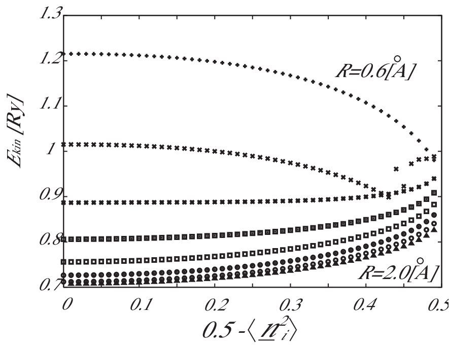

Now, we have another expression for . Consider the minimizing of which gives and is the solution of Eq. (12). Then, we have,
| (23) | |||||
Thus we may write as,
| (24) |
This is another exact expression of the true total energy of the electron system. Note that the U term does not appear in the formula, although it affects . People might find that the above expression can be used to avoid the double counting problem. Let us evaluate within the approximation utilized in Sec. 6. Now, look at the kinetic energy for the Hydrogen molecule. (Figure 7) When , the value decreases with decreasing , which is controlled by increasing . Namely, the horizontal axis is the direction of increasing . This reduction in the kinetic energy is caused by expansion of the wavefunction in the real space. Actually, the Hartree term decreases and the electron-ion potential terms reduces their absolute values. In this range, as seen in the shift in the Hartree term, expands with increasing . Thus, we find that decreases in a weakly correlated regime () by increasing .
Let us compare the result with the cases with . In this region, increases by increasing U. If we look at , we see that the value does not change so much and is almost constant, when . This fact means that is nearly unchanged. What the U term does in this regime is that it only shift the internal fluctuation. Thus, the value of increases. Now look at the expression of Eq. (24). The true value of is estimated by adding the kinetic energy of an uncorrelated Fermion system , which has , and subtracting from . In this example, since is nearly unchanged against shift in for , for finite may be approximated by for . The result suggests that is almost unchanged by increasing , while the state becomes a correlated state.
On the other hand, if we detect decrease of by increasing , this suggests that minimizing of should be close to . We have an inequality, . Thus, evaluated for finite is nearly the same as . However, increases by introduction of . When we have the weakly correlated regime , the U term is not necessary for the proper description of the system.
As a result, we conclude that we can utilize -dependence of to detect occurrence of the Coulomb suppression in a correlated electron system. Once we have a properly designed method to estimate , EKSS works as a first-principles calculation method for the correlated electron system in general even without a reference calculation prepared for each individual problem. The target systems for EKSS include the Mott insulating state. Actually, we know a numerical algorithm[38] to obtain the Legendre transform,
7.2 A test for the Mott insulator
To test the conduction property of the system within DFT, we may be able to utilize the next technique of the momentum boost. Let us consider a twisted boundary condition for our simulation.
and () are the unit vectors and the length of a simulation cell. The density-functional theory holds for any fixed . Let us shift from zero to adiabatically and obtain the lowest energy eigen value . Then we can connect and draw a graph of as a function of .
According to the Kohn argument,[39] we can identify the Mott insulating state by looking at the period of , although we may see only the lowest edge of the whole . If formation of a gap in the flow of is detected by changing the lattice constant, for example, the system undergoes the Mott transition. Actually, a complete test using the one-dimensional Hubbard model showed the period for the half-filled band, that is useful for the characterization of the ground state.[40] If the system is described in the Kohn-Sham scheme with LDA, however, the period would not change from the value of a metallic state. This failure would be recovered by the introduction of the term in the Kohn-Sham scheme. If we ask the system to reproduce the local fluctuation, modification of the Kohn-Sham system naturally makes the system interacting. This is a way to model the stiffness of the Mott insulating state against the boost induced by the imaginative magnetic flux, which amounts to with the unit flux . The nature of the ground state is modified via a change in the charge fluctuation.
Acknowledgement
The authors are grateful for many occasions of discussion with many researchers. K.K. especially thanks professors, H. Aoki, S. Tsuneyuki, H. Kamimura, M. Tsukada, M. Imada, M. Ogata, A. Hasegawa, H. Akai, H. Katayama-Yoshida, H. Kasai, M. Higuchi, K. Higuchi, Y. Morikawa, J. Yamauchi, and doctors, T. Ogitsu, K. Kobayashi and, Mr. M. Takahashi. This work was supported by a Grant-in-Aid for Scientific Research in Priority Areas “Development of New Quantum Simulators and Quantum Design” (No. 17064006), the 21st century COE program “Core Research and Advanced Eduation Center for Materials Science and Nano Engineering”, Grants-in-Aid for Scientific Research (No. 15GS0213) and also by a Computational Nanoscience program “Grid Application Research in Nanoscience-National Research Grid Initiative (NAREGI)” of the Ministry of Education, Culture, Sports, Science, and Technology, Japan.
References
References
- [1] P. Hohenberg and W. Kohn, Phys. Rev. 136, B864 (1964).
- [2] W. Kohn and L. J. Sham, Phys. Rev. 140, A1133 (1965).
- [3] M. Levy, Proc. Natl. Acad. Sci. (U.S.A.) 76, 6062 (1979).
- [4] M. Levy, Phys. Rev. A 26, 1200 (1982).
- [5] E. Lieb, Int. J. Quantum. Chem. 24, 243 (1983).
- [6] N. Hadjisavvas and A. Theophilou, Phys. Rev. A 30, 2183 (1984).
- [7] E.S. Kryachko and E.V. Ludeña, Energy Density Functional Theory of Many-Electron Systems, Kluwer, (1986).
- [8] R.G. Parr and W. Yang, Density-Functional Theory of Atoms and Molecules, Plenum, (1989).
- [9] R.M. Dreizler and K.U. Gross, Density Functional Theory, Springer, (1990).
- [10] L.F. Mattheiss, Phys. Rev. Lett. 58, 1028 (1987).
- [11] J.Y. Freeman and J.-H. Xu, Phys. Rev. Lett. 58, 1035 (1987).
- [12] K. Takagahara and H. Harima and A. Yanase, Jpn. J. Appl. Phys. 26, L352 (1987).
- [13] T. Oguchi, Jpn. J. Appl. Phys. 26, L417 (1987).
- [14] W.E. Pickett and H. Krakauer and D.A. Papaconstantopoulos and L.L. Boyer, Phys. Rev. B. 35, 7252 (1987).
- [15] R.V. Kasowski and W.Y. Hsu and F. Herman, Solid State Commun. 63, 1077 (1987).
- [16] R.V. Kasowski and W.Y. Hsu and F. Herman, Phys. Rev. B 36, 7248 (1987).
- [17] J. Hubbard Proc. Roy. Soc. (London) A276, 238 (1963).
- [18] D. Baeriswyl and D.K. Campbell and J.M.P. Carmelo and F. Guinea and E. Louis, The Hubabrd Model, Plenum, (1995).
- [19] K. Yamaguchi, Chem. Phys. Lett. 68, 477 (1979).
- [20] G.C. Lie and E. Clementi, J. Chem. Phys. 60, 1275, 1288 (1974).
- [21] F. Moscardó and E. San-Fabiän, Phys. Rev. A 44, 1549 (1991).
- [22] B. Miehlich and H. Stoll and A. Savin, Mol. Phys. 91, 527 (1997).
- [23] J. Gräfenstein and D. Cremer, Chem. Phys. Lett. 316, 316 (2000).
- [24] J. Gräfenstein and D. Cremer, Mol. Phys. 103, 279 (2005).
- [25] S. Yamanaka and K. Nakata and T. Takada and K. Kusakabe and J.M. Ugalde and K. Yamaguchi, Chem. Lett. 35, 242 (2006).
- [26] K. Kusakabe, J. Phys. Soc. Jpn 70, 2038 (2001).
- [27] K. Kusakabe, cond-mat/0505703 (2005).
- [28] V.I. Anizimov and J. Zaanen and O.K. Andersen, Phys. Rev. B 44, 943 (1991).
- [29] I.V. Solovyev and P.H. Dederichs and V.I. Anisimov, Phys. Rev. B 50, 16861 (1994).
- [30] A.I. Liechtenstein and V.I. Anisimov and J. Zaanen, Phys. Rev. B 52, R5467 (1995).
- [31] J.E. Harriman, Phys. Rev. A 6, 680 (1981).
- [32] G.H. Wannier, Phys. Rev. 52, 191 (1937).
- [33] N. Marzari and D. Vanderbilt, Phys. Rev. B 56, 12847 (1997).
- [34] K. Kusakabe and M. Takahashi and N. Suzuki, Physica B, 378-380, 271 (2006).
- [35] M. Takahashi and K. Kusakabe and N. Suzuki, Proc. 28th Int. Conf. PHys. Semicon. (Wien), in press.
- [36] J.F. Perdew and Y. Wang, Phys. Rev. B 45, 13244 (1992).
- [37] N. Troullier and J.L. Martins, Phys. Rev. B 43, 1993 (1991).
- [38] K. Kusakabe, unpublished.
- [39] W. Kohn, Phys. Rev. 133, A171 (1964).
- [40] K. Kusakabe, J. Phys. Soc. Jpn. 66, 2075 (1997).