Preserving Monotonicity in Anisotropic Diffusion
Abstract
We show that standard algorithms for anisotropic diffusion based on centered differencing (including the recent symmetric algorithm) do not preserve monotonicity. In the context of anisotropic thermal conduction, this can lead to the violation of the entropy constraints of the second law of thermodynamics, causing heat to flow from regions of lower temperature to higher temperature. In regions of large temperature variations, this can cause the temperature to become negative. Test cases to illustrate this for centered asymmetric and symmetric differencing are presented. Algorithms based on slope limiters, analogous to those used in second order schemes for hyperbolic equations, are proposed to fix these problems. While centered algorithms may be good for many cases, the main advantage of limited methods is that they are guaranteed to avoid negative temperature (which can cause numerical instabilities) in the presence of large temperature gradients. In particular, limited methods will be useful to simulate hot, dilute astrophysical plasmas where conduction is anisotropic and the temperature gradients are enormous, e.g., collisionless shocks and disk-corona interface.
Keywords:
Anisotropic diffusion , Finite differencing1 Introduction
Anisotropic diffusion, in which the rate of diffusion of some quantity is faster in certain directions than others, occurs in many different physical systems and applications. Examples include diffusion in geological formations [13], thermal properties of structural materials and crystals [5], image processing [11, 4, 9], biological systems, and plasma physics. Diffusion Tensor Magnetic Resonance Imaging makes use of anisotropic diffusion to distinguish different types of tissue as a medical diagnostic [2]. In plasma physics, the collision operator gives rise to anisotropic diffusion in velocity space, as does the quasilinear operator describing the interaction of particles with waves [16]. In magnetized plasmas, thermal conduction can be much more rapid along the magnetic field line than across it; this will be the main application in mind for this paper.
Centered finite differencing is commonly used to implement anisotropic thermal conduction in fusion and astrophysical plasmas [6, 10, 14]. Methods based on finite differencing [6] and higher order finite elements [15] are able to simulate highly anisotropic thermal conduction (, where and are parallel and perpendicular conduction coefficients, respectively) in laboratory plasmas. “Symmetric” differencing introduced in [6] is particularly simple and has some desirable properties: perpendicular numerical diffusion is independent of parallel conduction coefficient , perpendicular numerical diffusion is small, and the numerical heat flux operator is self adjoint. While in the symmetric method the components of the heat flux are located at cell corners, they are located at the cell faces in the “asymmetric” method. The asymmetric method has been used to study convection in anisotropically conducting plasmas [10] and in simulations of collisionless accretion disks [14].
An important fact that has been overlooked is that the methods based on centered differencing can give heat fluxes inconsistent with the second law of thermodynamics, i.e., heat can flow from lower to higher temperatures. This accentuates temperature extrema and may result in negative temperatures at some grid points, causing numerical instabilities as the sound speed becomes imaginary. Also, in image processing applications it is required that no new spurious extrema are generated with anisotropic diffusion [11], making centered differencing unviable.
We show that both the symmetric and asymmetric methods can be modified so that temperature extrema are not accentuated. The components of the anisotropic heat flux consist of two contributions: the normal term and the transverse term (see §2). The normal term for the asymmetric method (like isotropic conduction) always gives heat flux from higher to lower temperatures, but the transverse term can be of any sign. The transverse term can be “limited” to ensure that temperature extrema are not accentuated. We use slope limiters, analogous to those used in second order methods for hyperbolic problems [19, 8], to limit the transverse heat fluxes. For the symmetric method, where primary heat fluxes are located at cell corners, both normal and transverse terms need to be limited. Limiting based on the entropy-like function () is also discussed.
Limiting introduces numerical diffusion in the perpendicular direction, and the desirable property of the symmetric method that perpendicular pollution is independent of no longer holds. The ratio of perpendicular numerical diffusion and the physical parallel conductivity with a Monotonized Central (MC; see [8] for a discussion of slope limiters) limiter is for a modest number of grid points ( in each direction). This clearly is not adequate for simulating laboratory plasmas which require because perpendicular numerical diffusion will swamp the true perpendicular diffusion. For laboratory plasmas the temperature profile is relatively smooth and the negative temperature problem does not arise, so symmetric differencing [6] or higher order finite elements [15] may be adequate. However, astrophysical plasmas can have sharp temperature gradients, e.g., the transition region of the sun separating the hot corona and the much cooler chromosphere, or the disk-corona interface in accretion flows. In these applications centered differencing may lead to negative temperatures giving rise to numerical instabilities. Limiting introduces somewhat larger perpendicular numerical diffusion but will ensure that heat flows in the correct direction at temperature extrema; hence negative temperatures are avoided. Even a modest anisotropy in conduction () should be enough to study the qualitatively new effects of anisotropic conduction on dilute astrophysical plasmas [10], but the positivity of temperature is absolutely essential for numerical robustness.
The paper is organized as follows. In §2 we describe the heat equation with anisotropic conduction and its numerical implementation using asymmetric and symmetric centered differencing. In §3 we present simple test problems for which centered differencing results in negative temperatures. Limiting as a method to avoid unphysical behavior at temperature extrema is introduced in §4 & §5. Slope limiters are discussed in §4 and limiting based on the entropy-like condition in §5. Some mathematical properties of limited methods are discussed in §6. In §7 we compare different methods and their convergence properties with some test problems. We conclude in §8.
2 Anisotropic thermal conduction
Thermal conduction in plasmas with the mean free path much larger than the gyroradius is anisotropic with respect to the magnetic field lines; heat flows primarily along the field lines with little conduction in the perpendicular direction [3]. In such cases, a divergence of anisotropic heat flux is added to the energy equation. Thermal conduction can modify the characteristic structure of the magnetohydrodynamic (MHD) equations making it difficult to incorporate into upwind methods. However, thermal conduction can be evolved independently of the MHD equations using operator splitting, as done in [10]. The equation for the evolution of internal energy density due to anisotropic thermal conduction is
| (1) | |||||
| (2) |
where is the internal energy per unit volume, is the heat flux, and are the coefficients of parallel and perpendicular conduction with respect to the local field direction (with dimensions ), is the number density, is the temperature with as the ratio of specific heats for an ideal gas, is the unit vector along the field line, and represents the derivative along the magnetic field direction. Throughout the paper we use to avoid factors of and ; results of the paper are not affected by this choice.

We consider a staggered grid with the scalars like , , and located at the cell centers and the components of vectors, e.g., and , located at the cell faces [17], as shown in Figure 1. The face centered components of vectors naturally represent the flux of scalars out of a cell. All the methods presented here are conservative and fully explicit. It should be possible to take longer time steps with an implicit generalization of the schemes discussed in the paper, but the construction of fast implicit schemes for anisotropic conduction is non-trivial.
In two dimensions the internal energy density is updated as follows,
| (3) |
where the time step , satisfies the stability condition [12] (ignoring density variations)
| (4) |
and are grid sizes in the two directions. The generalization to three dimensions is straightforward.
The methods we discuss differ in the way heat fluxes are calculated at the faces. In rest of the section we discuss the methods based on asymmetric and symmetric centered differencing as discussed in [6]. From here on will represent parallel conduction coefficient in cases where an explicit perpendicular diffusion is not considered (i.e., the only perpendicular diffusion is due to numerical effects).
2.1 Centered asymmetric scheme

The heat flux in the - direction (in 2-D), using the asymmetric method is given by
| (5) |
where overline represents the variables interpolated to the face at . The variables without an overline are naturally located at the face. The interpolated quantities at the face are given by simple arithmetic averaging,
| (6) | |||||
| (7) |
We use a harmonic mean to interpolate the product of number density and conductivity [7],
| (8) |
this is second order accurate for smooth regions, but becomes proportional to the minimum of the two ’s on either side of the face when the two differ significantly. Figure 2 gives the motivation for using a harmonic average. Physically, using a harmonic average preserves the robust result that the heat flux into a region should go to zero as the density in that region goes to zero, as in a thermos bottle using a vacuum for insulation. Harmonic averaging is also necessary for the method to be stable with the time step in Eq. (4). Instead, if we use a simple mean, the stable time step condition becomes severe by a factor , which can result in an unacceptably small time step for initial conditions with a large density contrast. Physically, this is because the heat capacity is very small in low density regions, so even a tiny heat flux into that region causes rapid changes in temperature. Analogous expressions can be written for heat flux in other directions.
2.2 Centered symmetric scheme
The notion of symmetric differencing was introduced in [6], where primary heat fluxes are located at the cell corners, with
| (9) |
where overline represents the interpolation of variables at the corner given by a simple arithmetic average,
| (10) | |||||
| (11) | |||||
| (12) | |||||
| (13) |
As before (and for the same reasons), a harmonic average is used for the interpolation of ,
| (14) |
Analogous expressions can be written for . The harmonic average here is different from [6], who use an arithmetic average. Ref. [6] is primarily interested in magnetic fusion applications, where density variations are usually well resolved (shocks are usually not important in magnetic fusion) so arithmetic averaging will work well. But there might be some magnetic fusion cases, such as instabilities in the edge region of a fusion device, where there might be large density variations per grid cell and a harmonic average could be useful. All of the test cases in [6] used a uniform density and so will not be affected by the choice of arithmetic or harmonic average.
The heat fluxes located at the cell faces, and , to be used in Eq. (3) are given by an arithmetic average,
| (15) | |||||
| (16) |
As demonstrated in [6], the symmetric heat flux satisfies the self adjointness property (equivalent to ) at cell corners and has the desirable property that the perpendicular numerical diffusion () is independent of (see Figure 6 in [6]). But, as we show later, both symmetric and asymmetric schemes do not satisfy the crucial local property that heat must flow from higher to lower temperatures, the violation of which may result in negative temperature with large temperature gradients.
The heat flux in the - direction consists of two terms: the normal term and the transverse term . The asymmetric scheme uses a 2 point stencil to calculate the normal gradient and a 6 point stencil to calculate the transverse gradient, as compared to the symmetric method that uses a 6 point stencil for both (hence the name symmetric). This makes the symmetric method less sensitive to the orientation of coordinate system with respect to the field lines.

A problem with the symmetric method which is immediately apparent is its inability to diffuse away a chess-board temperature pattern as and , located at the cell corners, vanish for this initial condition (see Figure 3).
3 Negative temperature with centered differencing
In this section we present two simple test problems that demonstrate that negative temperatures can arise with both asymmetric and symmetric centered differencing.
3.1 Asymmetric method


Consider a grid with a hot zone () in the first quadrant and cold temperature () in the rest, as shown in Figure 4. Magnetic field is uniform over the box with . Number density is a constant equal to unity. Reflecting boundary conditions are used for temperature. Using the asymmetric scheme for heat fluxes out of the grid point (the third quadrant) gives, , and (where is assumed). Thus, heat flows out of the grid point , which is already a temperature minimum. This results in the temperature becoming negative. Figure 4 shows the temperature in the third quadrant vs. time for different methods. The asymmetric method gives negative temperature () for first few time steps, which eventually becomes positive. All other methods (except the one based on entropy limiting) give positive temperatures at all times for this problem. Methods based on limited temperature gradients will be discussed later. This test demonstrates that the asymmetric method may not be suitable for problems with large temperature gradients because negative temperature results in numerical instabilities.
3.2 Symmetric method


The symmetric method does not give negative temperature with the test problem of the previous section. In fact, the symmetric method gives the correct result for temperature with no numerical diffusion in the perpendicular direction (zero heat flux out of the grid point , see Figure 4). Other methods resulted in a temperature increase at because of perpendicular numerical diffusion. Here we consider a case where the symmetric method gives negative temperature.
As before, consider a grid with a hot zone () in the first quadrant and cold temperature () in the rest; the only difference from the previous test problem is that the magnetic field lines are along the - axis, and (see Figure 5). Reflective boundary conditions are used for temperature, as before. Since there is no temperature gradient along the field lines for the grid point , we do not expect the temperature there to change. While all other methods give a stationary temperature in time, the symmetric method results in a heat flux out of the grid through the corner at . With the initial condition as shown in Figure 5, the only non-vanishing symmetric heat flux out of is, . The only non-vanishing face-centered heat flux entering the box through a face is ; i.e., heat flows out of which is already a temperature minimum. This results in the temperature becoming negative at , although at late times it becomes equal to the initial temperature at . This simple test shows that the symmetric method can also give negative temperatures (and associated numerical problems) in presence of large temperature gradients.
4 Slope limited fluxes
As discussed earlier, the heat flux is composed of two terms: the normal term, and the transverse term. For the asymmetric method the discrete form of the term has the same sign as , and hence guarantees that heat flows from higher to lower temperatures. However, can have an arbitrary sign, and can give rise to heat flowing in the “wrong” direction. We use slope limiters, analogous to those used for linear reconstruction of variables in numerical simulation of hyperbolic systems [19, 8], to “limit” the transverse terms. Both asymmetric and symmetric methods can be modified with slope limiters. The slope limited heat fluxes ensure that temperature extrema are not accentuated. Thus, unlike the symmetric and asymmetric methods, slope limited methods can never give negative temperatures.
4.1 Limiting the asymmetric method
Since the normal heat flux term is naturally located at the face, no interpolation for is required for its evaluation. However, an interpolation at the - face is required to evaluate used in (the term with overlines in Eq. 5). The arithmetic average used in Eq. (7) for to calculate was found to result in heat flowing from lower to higher temperatures (see Figure 4). To remedy this problem we use slope limiters to interpolate temperature gradients in the transverse heat flux term.
Slope limiters are widely used in numerical simulations of hyperbolic equations (e.g., computational gas dynamics; see [19, 8]). Given the initial values for variables at grid centers, slope limiters (e.g., minmod, van Leer, and Monotonized Central (MC)) are used to calculate the slopes of conservative piecewise linear reconstructions in each grid cell. Limiters use the variable values in the nearest grid cells to come up with slopes that ensure that no new extrema are created for the conserved variables along the characteristics, a property of hyperbolic equations. Similarly, we use slope limiters to interpolate temperature gradients in the transverse heat flux term so that unphysical oscillations do not arise at temperature extrema.
The slope limited asymmetric heat flux in the - direction is still given by Eq. (5), with the same as in the asymmetric method, but a slope limited interpolation for the transverse temperature gradient , given by
| (17) | |||||
where is a slope limiter like minmod, van Leer, or Monotonized Central (MC) limiter [8]; e.g., the MC limiter is given by
| (18) |
where
A slope limiter weights the interpolation towards the argument smallest in magnitude, if the arguments differ by too much, and returns a zero if the two arguments are of opposite signs. An analogous expression for the transverse temperature gradient at the - face, , is used to evaluate the heat flux . Interpolation similar to the asymmetric method is used for all other variables (Eqs. 6 & 8).
4.2 Limiting the symmetric method
In the symmetric method, primary heat fluxes in both directions are located at the cell corners (see Eq. 9). Temperature gradients in both directions have to be interpolated at the corners. Thus, to ensure that temperature extrema are not amplified with the symmetric method, both and need to be limited.
The face-centered is calculated by averaging from the adjacent corners, which are given by the following slope-limited expressions:
| (19) | |||||
| (20) |
where and superscripts indicate the north-biased and south-biased heat fluxes. The face centered heat flux used in Eq. (3) is ; the other interpolated quantities (indicated with an overline) are the same as in Eq. (9). The limiter which is different from standard slope limiters is defined as
| (21) | |||||
where is a parameter; this reduces to a simple averaging if the temperature is smooth, while restricting the interpolated temperature () to not differ too much from (and be of the same sign). We choose for all of the results in this paper. Note that the limiter is not symmetric with respect to its arguments. It ensures that is of the same sign as ; i.e., the interpolated normal heat flux is from higher to lower temperatures. This interpolation will be able to diffuse the chess board pattern in Figure 3. The transverse temperature gradient is limited in a way similar to the asymmetric method; the temperature gradient is still given by Eq. (17). Thus if , the limited symmetric method becomes somewhat similar to the limited asymmetric method (though with differences in the interpolation of the magnetic field direction and of ).
5 Limiting with the entropy-like source function
If the entropy-like source function, which we define as (see Appendix A to see how this is different from the entropy function) is positive everywhere, heat is guaranteed to flow from higher to lower temperatures. For the symmetric method, evaluated at the cell corners is positive definite, but this need not be true for interpolations at the cell faces; thus heat may flow from lower to higher temperatures. An entropy-like condition can be applied at all face-pairs to limit the transverse heat flux terms ( and ), such that
| (22) |
The limiter is used to calculate the normal gradients and at the faces, as in the slope limited symmetric method (see §4.2). The use of ensures that , and only the transverse terms and need to be reduced to satisfy Eq. (22). That is, if on evaluating at all four face pairs the entropy-like condition (Eq. 22) is violated, the transverse terms are reduced to make vanish. The attractive feature of the entropy limited symmetric method is that it reduces to the symmetric method (which has the smallest numerical diffusion of all the methods; see Figure 9) when Eq. (22) is satisfied. The hope is that limiting of transverse terms may prevent oscillations with large temperature gradients.
The problem with entropy limiting, unlike the slope limited methods, is that it does not guarantee that numerical oscillations at large temperature gradients will be absent (e.g, see Figures 4 and 7). For example, when , Eq. (22) is satisfied for arbitrary heat fluxes and . In such a case, transverse heat fluxes and can cause heat to flow in the “wrong” direction, causing unphysical oscillations at temperature extrema. However, this unphysical behavior occurs only for a few time steps, after which the oscillations are damped. The result is that the overshoots are not as pronounced and quickly decay with time, unlike in the asymmetric and symmetric methods (see Figures 6 & 7). Although temperature extrema can be accentuated by the entropy limited method, early on one can choose sufficiently small time steps to ensure that temperature does not become negative; this is equivalent to saying that the entropy limited method will not give overshoots at late times (see Figure 7 and Tables 1-4). This trick will not work for the centered symmetric and asymmetric methods where temperatures can be negative even at late times (see Figure 7).
To guarantee that temperature extrema are not amplified, in addition to entropy limiting at all points, one can also use slope limiting of transverse temperature gradients at extrema. This results in a method that does not amplify the extrema, but is more diffusive compared to just entropy limiting (see Figure 9). Because of the simplicity of slope limited methods and their desirable mathematical properties (discussed in the next section), they are preferred over the cumbersome entropy limited methods.
6 Mathematical properties
In this section we prove that the slope limited fluxes satisfy the physical requirement that temperature extrema are not amplified. Also discussed are global and local properties related to the entropy-like condition .
6.1 Behavior at temperature extrema
Slope limiting of both asymmetric and symmetric methods guarantees that temperature extrema are not amplified further, i.e., the maximum temperature does not increase and the minimum temperature does not decrease, as required physically. This ensures that the temperature is always positive and numerical problems because of imaginary sound speed do not arise. The normal heat flux in the asymmetric method () and the limited normal heat flux term in the symmetric method (Eqs. 19 and 20) allows the heat to flow only from higher to lower temperatures. Thus the terms responsible for unphysical behavior at temperature extrema are the transverse heat fluxes and . Slope limiters ensure that the transverse heat terms vanish at extrema and heat flows down the temperature gradient at those grid points.
The operator , where is a slope limiter like minmod, van Leer, or MC, is symmetric with respect to all its arguments, and hence can be written as . For the slope limiters considered here (minmod, van Leer, and MC), vanishes unless all four arguments have the same sign. At a local temperature extremum (say at ), the - (and -) face-centered slopes and (and and ) are of opposite signs, or at least one of them is zero. This ensures that the slope limited transverse temperature gradients ( and ) vanish (from Eq. 17). Thus, the heat fluxes are and at the temperature extrema, which are always down the temperature gradient. This ensures that temperature never decreases (increases) at a temperature minimum (maximum), and negative temperatures are avoided.
6.2 The entropy-like condition,
If the number density remains constant in time, then multiplying Eq. (1) with and integrating over all space gives
| (23) | |||||
assuming that the surface contributions vanish. This analytic constraint implies that volume averaged temperature fluctuations cannot increase in time. Locally it gives the entropy-like condition , implying that heat always flows from higher to lower temperatures.
Ref. [6] has shown that the symmetric method satisfies at cell corners. The entropy-like function evaluated at with the symmetric method is
| (24) |
Using the symmetric heat fluxes (Eq. 9) the entropy-like function becomes,
| (25) | |||||
and integration over the whole space implies Eq. (23). Although the entropy-like condition is satisfied by the symmetric method at grid corners (both locally and globally), this condition is not sufficient to guarantee positivity of temperature at cell centers, as we demonstrate in §3.2. Also notice that the modification of the symmetric method to satisfy the entropy-like condition at face pairs (see §5) does not cure the problem of negative temperatures (see Figure 4). Thus, a method which satisfies the entropy-like condition () interpolated at some point does not necessarily satisfy it everywhere, implying that unphysical oscillations in the presence of large temperature gradients may arise even if the interpolated entropy-like condition holds.
With an appropriate interpolation, the asymmetric method and the slope limited asymmetric methods can be modified to satisfy the global entropy-like condition . Consider
| (26) |
where and are the number of grid points in each direction. Substituting the form of asymmetric heat fluxes,
| (27) | |||||
where overlines represent appropriate interpolations. We define
| (28) | |||||
| (29) | |||||
| (30) | |||||
| (31) |
In terms of ’s, Eq. (27) can be written as
| (32) | |||||
A lower bound on is obtained by assuming the cross terms to be negative, i.e.,
| (33) | |||||
Now define and as follows (the following interpolation is necessary for the proof to hold):
| (34) | |||||
| (35) |
where is an arithmetic average (as in centered asymmetric method) or a slope limiter (e.g., minmod, van Leer, or MC) which satisfies the property that . Thus,
| (36) | |||||
Shifting the dummy indices and combining various terms give,
| (37) | |||||
Thus, an appropriate interpolation for the asymmetric and the slope limited asymmetric methods results in a scheme that satisfies the global entropy-like condition. A variation of this proof can be used to prove the global entropy condition by multiplying Eq. (1) with instead of (see Appendix A), although the form of interpolation would need to be modified slightly. It is comforting that introducing a limiter to the asymmetric method does not break the global entropy-like condition. However, it is important to remember that the entropy-like (or entropy) condition satisfied at some point does not guarantee a local heat flow in the correct direction; thus it is necessary to use slope limiters at temperature extrema to avoid temperature oscillations.
7 Further tests
| Method | L1 error | L2 error | L error | Tmax | Tmin | |
|---|---|---|---|---|---|---|
| asymmetric | 0.0324 | 0.0459 | 0.0995 | 10.0926 | 9.9744 | 0.0077 |
| asymmetric minmod | 0.0471 | 0.0627 | 0.1195 | 10.0410 | 10 | 0.0486 |
| asymmetric MC | 0.0358 | 0.0509 | 0.1051 | 10.0708 | 10 | 0.0127 |
| asymmetric van Leer | 0.0426 | 0.0574 | 0.1194 | 10.0519 | 10 | 0.0238 |
| symmetric | 0.0114 | 0.0252 | 0.1425 | 10.2190 | 9.9544 | 0.00028 |
| symmetric entropy | 0.0333 | 0.0477 | 0.0997 | 10.0754 | 10 | 0.0088 |
| symmetric entropy extrema | 0.0341 | 0.0487 | 0.1010 | 10.0751 | 10 | 0.0101 |
| symmetric minmod | 0.0475 | 0.0629 | 0.1322 | 10.0406 | 10 | 0.0490 |
| symmetric MC | 0.0289 | 0.0453 | 0.0872 | 10.0888 | 10 | 0.0072 |
| symmetric van Leer | 0.0438 | 0.0585 | 0.1228 | 10.0519 | 10 | 0.0238 |
The errors are based on the assumption that the initial hot patch has diffused to a uniform temperature () in the ring 0.50.7, and outside it.
| Method | L1 error | L2 error | L error | Tmax | Tmin | |
|---|---|---|---|---|---|---|
| asymmetric | 0.0256 | 0.0372 | 0.0962 | 10.1240 | 9.9859 | 0.0030 |
| asymmetric minmod | 0.0468 | 0.0616 | 0.1267 | 10.0439 | 10 | 0.0306 |
| asymmetric MC | 0.0261 | 0.0405 | 0.0907 | 10.1029 | 10 | 0.0040 |
| asymmetric van Leer | 0.0358 | 0.0502 | 0.1002 | 10.0741 | 10 | 0.0971 |
| symmetric | 0.0079 | 0.0173 | 0.1206 | 10.2276 | 9.9499 | |
| symmetric entropy | 0.0285 | 0.0420 | 0.0881 | 10.0961 | 10 | 0.0042 |
| symmetric entropy extrema | 0.0291 | 0.0425 | 0.0933 | 10.0941 | 10 | 0.0041 |
| symmetric minmod | 0.0471 | 0.0618 | 0.1275 | 10.0433 | 10 | 0.0305 |
| symmetric MC | 0.0123 | 0.0252 | 0.1133 | 10.1406 | 10 | 0.00084 |
| symmetric van Leer | 0.0374 | 0.0514 | 0.1038 | 10.0697 | 10 | 0.0104 |
| Method | L1 error | L2 error | L error | Tmax | Tmin | |
|---|---|---|---|---|---|---|
| asymmetric | 0.0165 | 0.0281 | 0.0949 | 10.1565 | 9.9878 | 0.0012 |
| asymmetric minmod | 0.0441 | 0.0585 | 0.1214 | 10.0511 | 10 | 0.0191 |
| asymmetric MC | 0.0161 | 0.0289 | 0.0930 | 10.1397 | 10 | 0.0015 |
| asymmetric van Leer | 0.0264 | 0.0407 | 0.0928 | 10.1006 | 10 | 0.0035 |
| symmetric | 0.0052 | 0.0132 | 0.1125 | 10.2216 | 9.9509 | |
| symmetric entropy | 0.0256 | 0.0385 | 0.0959 | 10.1103 | 10 | 0.0032 |
| symmetric entropy extrema | 0.0260 | 0.0391 | 0.0954 | 10.1074 | 10 | 0.0032 |
| symmetric minmod | 0.0444 | 0.0588 | 0.1219 | 10.0503 | 10 | 0.0192 |
| symmetric MC | 0.0053 | 0.0160 | 0.0895 | 10.1676 | 10 | 0.0002 |
| symmetric van Leer | 0.0281 | 0.0426 | 0.0901 | 10.0952 | 10 | 0.0038 |
| Method | L1 error | L2 error | L error | Tmax | Tmin | |
|---|---|---|---|---|---|---|
| asymmetric | 0.0118 | 0.0234 | 0.0866 | 10.1810 | 9.9898 | |
| asymmetric minmod | 0.0399 | 0.0539 | 0.1120 | 10.0629 | 10 | 0.0115 |
| asymmetric MC | 0.0102 | 0.0230 | 0.0894 | 10.1708 | 10 | |
| asymmetric van Leer | 0.0167 | 0.0290 | 0.1000 | 10.1321 | 10 | 0.0013 |
| symmetric | 0.0033 | 0.0104 | 0.1112 | 10.2196 | 9.9504 | |
| symmetric entropy | 0.0252 | 0.0384 | 0.0969 | 10.1144 | 10 | 0.0027 |
| symmetric entropy extrema | 0.0253 | 0.0383 | 0.0958 | 10.1135 | 10 | 0.0026 |
| symmetric minmod | 0.0401 | 0.0541 | 0.1124 | 10.0622 | 10 | 0.0116 |
| symmetric MC | 0.0032 | 0.0122 | 0.0896 | 10.1698 | 10 | |
| symmetric van Leer | 0.0182 | 0.0307 | 0.1026 | 10.1260 | 10 | 0.0013 |
We use test problems discussed in [10] and [15] to compare different methods. The first test problem (taken from [10]) initializes a hot patch in circular field lines; ideally the hot patch should diffuse only along the field lines, but perpendicular numerical diffusion causes some cross-field thermal conduction. Unlike the limited methods, both asymmetric and symmetric methods show temperature oscillations at the temperature discontinuity. The second test problem (from [15]) includes a source term and an explicit perpendicular diffusion coefficient (). The steady state temperature gives a measure of the perpendicular numerical diffusion .
7.1 Diffusion of a hot patch in circular magnetic field


The circular diffusion test problem was proposed in [10]. A hot patch surrounded by a cooler background is initialized in circular field lines; the temperature drops discontinuously across the patch boundary. At late times, we expect the temperature to become uniform (and higher) in a ring along the magnetic field lines. The computational domain is a Cartesian box. The initial temperature distribution is given by
| (38) | |||||
where and . Fixed circular magnetic field lines centered at the origin are initialized and number density () is set to unity. Reflective boundary conditions are used for temperature; magnetic field and conduction vanishes outside . The parallel conduction coefficient ; there is no explicit perpendicular diffusion (). We evolve the anisotropic conduction equation (3) till time = 200, by when we expect the temperature to be almost uniform along the circular ring . In steady state (at late times), energy conservation implies that the ring temperature should be 10.1667, while the temperature outside the ring should be maintained at 10.
Figure 6 shows the temperature distribution for different methods at time=200. All methods result in a higher temperature in the annulus . The limited schemes show larger perpendicular diffusion (see Tables 1-4 which give errors, minimum and maximum temperatures, and numerical perpendicular diffusion at time=200; also see Figure 8) compared to the symmetric and asymmetric schemes. The perpendicular numerical diffusion () scales with the parallel diffusion coefficient for all methods. Notice that for Sovinec’s test problem (discussed in the next section) where temperature is smooth and an explicit is present, perpendicular numerical diffusion for the symmetric method does not increase with increasing .
The minmod limiter is much more diffusive than van Leer and MC limiters. Both symmetric and asymmetric methods give a minimum temperature below the initial minimum of 10, even at late times. At late times the symmetric method gives a temperature profile full of non-monotonic oscillations (Figure 6). Although the slope limited fluxes are more diffusive than the symmetric and asymmetric methods, they never show undershoots below the minimum temperature. The entropy limited symmetric method gives temperature undershoots at early times which are damped quickly, and the minimum temperature is still at late times (see Tables 1-4 & Figure 7). Entropy limiting combined with a slope limiter at temperature extrema behaves similar to the slope limiter based schemes.

Strictly speaking, a hot ring surrounded by a cold background is not a steady solution for the ring diffusion problem. Temperature in the ring will diffuse in the perpendicular direction (because of perpendicular numerical diffusion, although very slowly) until the whole box is at a constant temperature. A rough estimate for time averaged perpendicular numerical diffusion follows from Eq. (1),
| (39) |
where the space integral is taken over the hot ring , and and are the initial and final temperature distributions in the ring. Figure 8 plots the numerical perpendicular diffusion (using Eq. 39) for the ring diffusion problem at different resolutions (see Tables 1-4). The estimates for perpendicular diffusion agree roughly with the more accurate calculations using Sovinec’s test problem described in the next section (compare Figures 8 & 9); as with Sovinec’s test, the symmetric method is the least diffusive. Table 5 lists the convergence rate of for the ring diffusion problem evolved with different methods.
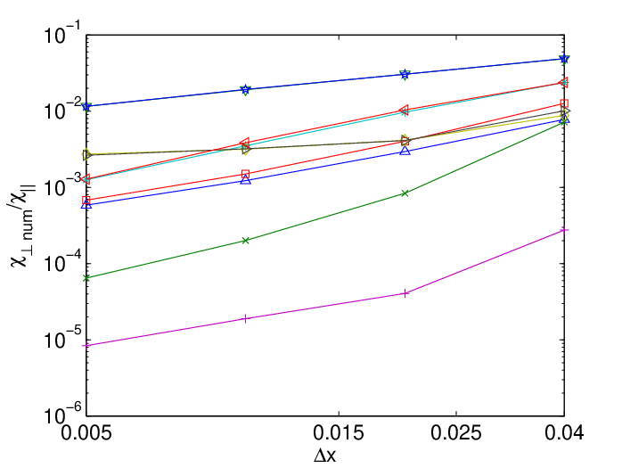
| Method | slope |
|---|---|
| asymmetric | 1.066 |
| asymmetric minmod | 0.741 |
| asymmetric MC | 1.142 |
| asymmetric van Leer | 1.479 |
| symmetric | 1.181 |
| symmetric entropy | 0.220 |
| symmetric entropy extrema | 0.282 |
| symmetric minmod | 0.735 |
| symmetric MC | 1.636 |
| symmetric van Leer | 1.587 |
To study the very long time behavior of different methods (in particular to check whether the symmetric and asymmetric methods give negative temperatures even at very late times) we initialize the same problem with the hot patch at 10 and the cooler background at 0.1. Figure 7 shows the minimum temperature with time for the symmetric, asymmetric, and entropy limited symmetric methods; slope limited methods give the correct result for the minimum temperature () at all times. With a large temperature contrast, both symmetric and asymmetric methods give negative minimum temperature even at late times. Such points where temperature becomes negative, when coupled with MHD equations, can give numerical instabilities because of an imaginary sound speed. The minimum temperature with the entropy limited symmetric method shows small undershoots at early times which are damped quickly and the minimum temperature is equal to the initial minimum () after time=1.
7.2 Convergence studies: measuring


We use the steady state test problem described in [15] to measure the perpendicular numerical diffusion coefficient, . The computational domain is a unit square , with vanishing temperature at the boundaries; number density is set to unity. The source term that drives the lowest eigenmode of the temperature distribution is added to Eq. (1). The anisotropic diffusion equation with a source term possesses a steady state solution. The equation that we evolve is
| (40) |
The magnetic field is derived from the flux function of the form ; this results in concentric field lines centered at the origin. The temperature eigenmode driven by the source function is constant along the field lines. The steady state solution for the temperature is , independent of . The perpendicular diffusion coefficient is chosen to be unity, thus gives a measure of total perpendicular diffusion: the sum of (the explicit perpendicular diffusion) and (the perpendicular numerical diffusion).
To account for due to the errors in discretization of the parallel diffusion operator, we calculate , where is the central temperature calculated by the discretized equations at the same resolution in the isotropic limit . The convention that we use is slightly different (and more accurate) than that used in previous work, , which effectively assumed that isotropic diffusion gives exactly.
Figure 9 shows the perpendicular numerical diffusivity for , using different methods. The perpendicular diffusion () for all methods except the symmetric method increases linearly with . This property has been emphasized by [6] to motivate the use of symmetric differencing for fusion applications, which require the perpendicular numerical diffusion to be small for . The slope limited methods (with a reasonable resolution) are not suitable for the applications which require ; this rules out the fusion applications mentioned in [6, 15]. However, only the slope limited methods give physically appropriate behavior at temperature extrema, thereby avoiding negative temperatures in presence of sharp temperature gradients. The error (perpendicular numerical diffusion, ) for most methods except the ones based on minmod limiter, show a roughly second order convergence (see Table 6).
| Method | ||
|---|---|---|
| asymmetric | 1.802 | 1.770 |
| asymmetric minmod | 0.9674 | 0.9406 |
| asymmetric MC | 1.9185 | 1.9076 |
| asymmetric van Leer | 1.706 | 1.728 |
| symmetric | 1.726 | 1.762 |
| symmetric entropy | 2.407 | 2.966 |
| symmetric entropy extrema | 1.949 | 1.953 |
| symmetric minmod | 0.9155 | 0.8761 |
| symmetric MC | 1.896 | 1.9049 |
| symmetric van Leer | 1.6041 | 1.6440 |
8 Conclusions
It is shown that simple centered differencing of anisotropic conduction can result in negative temperatures in the presence of large temperature gradients. We present simple test problems where asymmetric and symmetric methods give heat flowing from lower to higher temperatures, leading to negative temperatures at some grid points. Negative temperature results in numerical instabilities, as the sound speed becomes imaginary. Numerical schemes based on slope limiters are proposed to solve this problem.
The methods developed here will be useful in numerical studies of hot, dilute, anisotropic astrophysical plasmas [10, 14], where large temperature gradients may be common. Anisotropic conduction can play a crucial role in determining the global structure of hot, non-radiative accretion flows (e.g., [1, 10, 14]). Therefore, it will be useful to extend ideal MHD codes used in previous global numerical studies (e.g., [18]) to include anisotropic conduction. Slope limiting methods that prevent negative temperature can be particularly helpful in global disk simulations where there are huge temperature gradients that occur between a hot, dilute corona and the cold, dense disk. The slope limited method with an MC limiter appears to be the most accurate method that does not result in unphysical behavior with large temperature gradients (see Figures 6 & 8). While we have tried a number of possible variations other than the ones described here, there might be ways to further improve these algorithms. Future work might explore other combinations of limiters, or limiters on combined fluxes instead of limiting the normal and transverse components independently, or might explore using higher-order information to reduce the effects of limiters near extrema while preserving physical behavior.
Although the slope and entropy limited methods in the present form are not suitable for fusion applications that require accurate resolution of perpendicular diffusion for huge anisotropy (), they are appropriate for astrophysical applications with large temperature gradients. A relatively small anisotropy of thermal conduction may be sufficient to study the effects of anisotropic thermal conduction [10]. The primary advantage of the limited methods is their robustness in presence of large temperature gradients. Apart from the simulations of dilute astrophysical plasmas with large temperature gradients (e.g., magnetized collisionless shocks), monotonicity-preserving methods may find use in diverse fields where anisotropic diffusion is important, e.g., image processing, biological transport, and geological systems.
9 Acknowledgments
Useful discussions with Tom Gardiner, Ian Parrish, and Ravi Samtaney are acknowledged. This work is supported by the US DOE under contract # DE-AC02-76CH03073 and the NASA grant NNH06AD01I.
Appendix A Entropy condition for an ideal gas
The entropy for an ideal gas is given by , where is the number density, V the volume, the temperature, and the ratio of specific heats ( for a 3-D mono-atomic gas). The change in entropy that results from adding an amount of heat to a uniform gas is
We measure temperature in energy units, so . The rate of change of entropy of a system where number density and temperature can vary in space (density is assumed to be constant in time) is given by
| (41) |
where we use an anisotropic heat flux, , and the integral is evaluated over the whole space with the boundary contributions assumed to vanish. The local entropy function defined as can be integrated to calculate the rate of change of total entropy of the system.
In the paper we use a related function (the entropy-like function ) defined as to limit the symmetric methods using face-pairs, and to prove some properties of different anisotropic diffusion schemes. The condition ensures that heat always flows from higher to lower temperatures.
References
- [1] S. A. Balbus, Convective and Rotational Stability of a Dilute Plasma, Astrophys. J. 562, 909 (2001).
- [2] P. J. Basser & D. K. Jones, Diffusion-Tensor MRI: Theory, Experimental Design, and Data Analysis—A Technical Review, NMR Biomed. 15, 456 (2002).
- [3] S. I. Braginskii, Reviews of Plasma Physics, Vol. 1, ed. M. A. Leontovich, Consultants Bureau, New York, 1965.
- [4] V. Caselles, J.M. Morel, G. Sapiro, & A. Tannenbaum, Introduction to the Special Issue on Partial Differential Equations and Geometry-Driven Diffusion in Image Processing and Analysis, IEEE Trans. on Image Processing 7, 269 (1998).
- [5] Z. Dian-lin et al., Anisotropic Thermal Conductivity of the 2D Single Quasicrystals: Ali65Ni20Co15 and Al62Si3Cu20Co15, Phys. Rev. Lett. 66, 2778 (1991).
- [6] S. Günter, Q. Yu, J. Kruger, & K. Lackner, Modelling of Heat Transport in Magnetised Plasmas Using Non-Aligned Coordinates, J. Comput. Phys. 209, 354 (2005).
- [7] J. Hyman, J. Morel, M. Shashkov, & S. Steinberg, Mimetic Finite Difference Methods for Diffusion Equations, Computational Geosciences 6, 333 (2002).
- [8] R. J. Leveque, Finite Volume Methods for Hyperbolic Problems, Cambridge Univ. Press, 2002.
- [9] P. Mrázek & M. Navara, Consistent Positive Directional Splitting of Anisotropic Diffusion, Proc. of Computer Vision Winter Workshop, Bled, Slovenia, Feb. 7-9, 37 (2001).
- [10] I. J. Parrish & J. M. Stone, Nonlinear Evolution of the Magnetothermal Instability in Two Dimensions, Astrophys. J. 633, 334 (2005).
- [11] P. Perona & J. Malik, Scale-Space and Edge Detection Using Anisotropic Diffusion, IEEE Trans. on Pattern Analysis and Machine Intelligence 12, 629 (1990).
- [12] R. D. Richtmyer & K. W. Morton, Difference Methods for Initial-value Problems, Interscience Publishers, New York, 1967.
- [13] M. Saadatfar & M. Sahimi, Diffusion in Disordered Media With Long-Range Correlations: Anomalous, Fickian, and Superdiffusive Transport and Log-Periodic Oscillations, Phys. Rev. B 65, 036116 (2002).
- [14] P. Sharma, G. W. Hammett, E. Quataert & J. M. Stone, Shearing Box Simulations of the MRI in a Collisionless Plasma, Astrophys. J. 637, 952 (2006).
- [15] C. R. Sovinec & the NIMROD Team, Nonlinear Magnetohydrodynamics Simulation Using High-Order Finite Elements, J. Comput. Phys. 195, 355 (2004).
- [16] T. H. Stix, Waves in Plasmas, Amer. Inst. of Phys., New York, 1992.
- [17] J. M. Stone & M. L. Norman, ZEUS-2D: A Radiation Magnetohydrodynamics Code for Astrophysical Flows in Two Space Dimensions. I – The Hydrodynamic Algorithms and Tests, Astrophys. J. Supp., 80, 753 (1992).
- [18] J. M. Stone & J. E. Pringle, Magnetohydrodynamical Non-Radiative Accretion Flows in Two Dimensions, Monthly Notices of the Royal Astronomical Society 322, 461 (2001).
- [19] B. van Leer, Towards the Ultimate Conservative Difference Scheme V., A Second Order Sequel to Gudonov’s Method, J. Comput. Phys. 32, 101 (1979).