The Refractive Index of Curved Spacetime: the Fate of Causality in QED
Abstract:
It has been known for a long time that vacuum polarization in QED leads to a superluminal low-frequency phase velocity for light propagating in curved spacetime. Assuming the validity of the Kramers-Kronig dispersion relation, this would imply a superluminal wavefront velocity and the violation of causality. Here, we calculate for the first time the full frequency dependence of the refractive index using world-line sigma model techniques together with the Penrose plane wave limit of spacetime in the neighbourhood of a null geodesic. We find that the high-frequency limit of the phase velocity (i.e. the wavefront velocity) is always equal to and causality is assured. However, the Kramers-Kronig dispersion relation is violated due to a non-analyticity of the refractive index in the upper-half complex plane, whose origin may be traced to the generic focusing property of null geodesic congruences and the existence of conjugate points. This puts into question the issue of micro-causality, i.e. the vanishing of commutators of field operators at spacelike separated points, in local quantum field theory in curved spacetime.
1 Introduction
Quantum field theory in curved spacetime is by now a well-understood subject. However, there remain a number of intriguing puzzles which hint at deeper conceptual implications for quantum gravity itself. The best known is of course Hawking radiation and the issue of entropy and holography in quantum black hole physics. A less well-known effect is the discovery by Drummond and Hathrell [2] that vacuum polarization in QED can induce a superluminal phase velocity for photons propagating in a non-dynamical, curved spacetime. The essential idea is illustrated in Figure 1. Due to vacuum polarization, the photon may be pictured as an electron-positron pair, characterized by a length scale , the Compton wavelength of the electron. When the curvature scale becomes comparable to , the photon dispersion relation is modified. The remarkable feature, however, is that this modification can induce a superluminal11 1 In this paper, we use the term “superluminal” in the sense “greater than ”. Apart from the occasional use of in the text for clarity, we set throughout. Also, in our conventions, the metric of flat space is and the Riemann tensor is . low-frequency phase velocity, i.e. the photon momentum becomes spacelike.

At first, it appears that this must be incompatible with causality. However, as discussed in refs. [3, 4, 5], the relation of causality with the “speed of light” is far more subtle. For our purposes, we may provisionally consider causality to be the requirement that no signal may travel faster than the fundamental constant defining local Lorentz invariance. More precisely, we require that the wavefront velocity , defined as the speed of propagation of a sharp-fronted wave pulse, should be less than, or equal to, . Importantly, it may be shown [6, 3, 5] that , the high-frequency limit of the phase velocity. In other words, causality is safe even if the low-frequency22 2 The term “low frequency” in this context requires some clarification. We work throughout in the WKB short wavelength approximation and in the limit of weak curvature where is a characteristic curvature of the background (which can also include derivatives of the curvature) and is the electron mass. The frequency enters in the dimensionless ration and when we talk about “low” and “high” frequency we really mean small and large values of this dimensionless parameter. phase velocity is superluminal provided the high-frequency limit does not exceed .
This appears to remove the potential paradox associated with a superluminal . However, a crucial constraint is imposed by the Kramers-Kronig dispersion relation33 3 Note that we are using “dispersion relation” in two different senses here. For clarity, we will always refer to eq.(1) explicitly as the Kramers-Kronig or KK dispersion relation to distinguish it from the use of the term dispersion relation to describe the frequency dependence of the photon light-cone. (see, e.g. ref. [7], chpt. 10.8) for the refractive index, viz.
| (1) |
where . The positivity of , which is true for an absorptive medium and is more generally a consequence of unitarity in QFT, then implies that , i.e. . So, given the validity of the KK dispersion relation, a superluminal would imply a superluminal wavefront velocity with the consequent violation of causality.
We are therefore left with three main options [5], each of which would have dramatic consequences for our established ideas about quantum field theory:
Option (1) The wavefront speed of light and the physical light cones lie outside the geometric null cones of the curved spacetime, in apparent violation of causality.
It should be noted, however, that while this would certainly violate causality for theories in Minkowski spacetime, it could still be possible for causality to be preserved in curved spacetime if the effective metric characterizing the physical light cones defined by nevertheless allow the existence of a global timelike Killing vector field. This possible loophole exploits the general relativity notion of “stable causality” [9, 10] and is discussed further in ref. [3].
Option (2) Curved spacetime may behave as an optical medium exhibiting gain, i.e. .
This possibility was explored in the context of -systems in atomic physics in ref.[5], where laser-atom interactions can induce gain, giving rise to a negative and superluminal low-frequency phase velocities while preserving and the KK dispersion relation. However, the problem in extending this idea to QFT is that the optical theorem, itself a consequence of unitarity, identifies the imaginary part of forward scattering amplitudes with the total cross section. Here, should be proportional to the cross section for pair creation and therefore positive. A negative would appear to violate unitarity.
Option (3) The Kramers-Kronig dispersion relation (1) is itself violated. Note, however, that this relation only relies on the analyticity of in the upper-half plane, which is usually considered to be a direct consequence of an apparently fundamental axiom of local quantum field theory, viz. micro-causality.
Micro-causality in QFT is the requirement that the expectation value of the commutator of field operators vanishes when and are spacelike separated. While this appears to be a clear statement of what we would understand by causality at the quantum level, in fact its primary rôle in conventional QFT is as a necessary condition for Lorentz invariance of the -matrix (see e.g. ref. [7], chpts. 5.1, 3.5). Since QFT in curved spacetime is only locally, and not globally, Lorentz invariant, it is just possible there is a loophole here allowing violation of micro-causality in curved spacetime QFT.
Despite these various caveats, unitarity, micro-causality, the identification of light cones with geometric null cones and causality itself are all such fundamental elements of local relativistic QFT that any one of these options would represent a major surprise and pose a severe challenge to established wisdom. Nonetheless, it appears that at least one has to be true.
To understand how QED in curved spacetime is reconciled with causality, it is therefore necessary to perform an explicit calculation to determine the full frequency dependence of the refractive index in curved spacetime. This is the technical problem which we solve in this paper. The remarkable result is that QED chooses option (3), viz. analyticity is violated in curved spacetime. We find that in the high-frequency limit, the phase velocity always approaches , so we determine . Moreover, we are able to confirm that where the background gravitational field induces pair creation, , is indeed positive as required by unitarity. However, the refractive index is not analytic in the upper half-plane, and the KK dispersion relation is modified accordingly. One might think that this implies a violation of microcausality, however, there is a caveat in this line of argument which requires a more ambitious off-shell calculation to settle definitively [8].
In order to establish this result, we have had to apply radically new techniques to the analysis of the vacuum polarization for QED in curved spacetime. The original Drummond-Hathrell analysis was based on the low-energy, effective action for QED in a curved background,
| (2) |
derived using conventional heat-kernel or proper-time techniques (see, for example, [11, 12, 13, 14, 15]. A geometric optics, or eikonal, analysis applied to this action determines the low-frequency limit of the phase velocity. Depending on the spacetime, the photon trajectory and its polarization, may be superluminal [2, 16, 17]. In subsequent work, the expansion of the effective action to all orders in derivatives, but still at , was evaluated and applied to the photon dispersion relation [12, 13, 18, 19]. However, as emphasized already in refs. [3, 4, 19], the derivative expansion is inadequate to find the high-frequency behaviour of the phase velocity. The reason is that the frequency appears in the on-shell vacuum polarization tensor only in the dimensionless ratio . The high-frequency limit depends non-perturbatively on this parameter44 4 Notice that here we also include derivatives of the curvature in the generic symbol “”. In fact, in ref. [19], the contribution to the on-shell vacuum polarization was determined in the form , where represents the variation of the curvature along the geodesic with tangent vector and the function is a form-factor determined from the effective action. This behaviour, where the vacuum polarization depends on the curvature through its variation , where is a light-cone coordinate adapted to the photon’s original null geodesic, is reflected in the form of the Penrose limit for general curved spacetimes: see Section 7. and so is not accessible to an expansion truncated at first order in .
In this paper, we instead use the world-line formalism which can be traced back to Feynman and Schwinger [20, 21], and which has been extensively developed in recent years into a powerful tool for computing Green functions in QFT via path integrals for an appropriate 1-dim world-line sigma model. (For a review, see e.g. ref. [22].) The power of this technique in the present context is that it enables us to calculate the QED vacuum polarization non-perturbatively in the frequency parameter using saddle-point techniques. Moreover, the world-line sigma model provides an extremely geometric interpretation of the calculation of the quantum corrections to the vacuum polarization. In particular, we are able to give a very direct interpretation of the origin of the Kramers-Kronig violating poles in in terms of the general relativistic theory of null congruences and the relation of geodesic focusing to the Weyl and Ricci curvatures via the Raychoudhuri equations.
A further key insight is that to leading order in , but still exact in , the relevant tidal effects of the curvature on photon propagation are encoded in the Penrose plane-wave limit [23, 24] of the spacetime expanded about the original null geodesic traced by the photon. This is a huge simplification, since it reduces the problem of studying photon propagation in an arbitrary background to the much more tractable case of a plane wave. In fact, the Penrose limit is ideally suited to this physical problem. As shown in ref. [25], where the relation with null Fermi normal coordinates is explained, it can be extended into a systematic expansion in a scaling parameter which for our problem is identified as . The Penrose expansion therefore provides us with a systematic way to go beyond leading order in curvature.
The paper is organized as follows. In Section 2, we introduce the world-line formalism and set up the geometric sigma model and eikonal approximation. The relation of the Penrose limit to the expansion is then explained in detail, complemented by a power-counting analysis in the appendix. The geometry of null congruences is introduced in Section 3, together with the simplified symmetric plane wave background in which we perform our detailed calculation of the refractive index. This calculation, which is the heart of the paper, is presented in Section 4. The interpretation of the result for the refractive index is given in Section 5, where we plot the frequency dependence of and prove that asymptotically . We also explain exactly how the existence of conjugate points in a null congruence leads to zero modes in the sigma model partition function, which in turn produces the KK-violating poles in in the upper half-plane. The implications for micro-causality are described in Section 6. Finally, in Section 7 we make some further remarks on the generality of our results for arbitrary background spacetimes before summarizing our conclusions in Section 8.
2 The World-Line Formalism

In the world-line formalism for scalar QED55 5 Since all the conceptual issues we address are the same for scalars and spinors, for simplicity we perform explicit calculations for scalar QED in this paper. The generalization of the world-line formalism to spinor QED is straightforward and involves the addition of a further, Grassmann, field in the path integral. For ease of language, we still use the terms electron and positron to describe the scalar particles. the 1-loop vacuum polarization is given by
| (3) |
The loop with the photon insertions is illustrated in Figure (2). The expectation value is calculated in the one-dimensional world-line sigma model involving periodic fields with an action
| (4) |
where is the mass of the (scalar) electron and we work in Minkowski signature in both spacetime and on the world-line.66 6 This will require some appropriate prescription. In particular, the integration contour should lie just below the real axis to ensure that the integral converges at infinity. The factor is the partition function of the world-line sigma model relative to flat space.77 7 In general, one has to introduce ghost fields to take account of the non-trivial measure for the fields, in curved spacetime [26, 27, 28, 29, 30]. However, in our calculation where we work to leading order in in a special set of coordinates the determinant factor is 1 to leading order. It is an important detail of our calculation that will depend implicitly on and the insertion points and .
The vertex operators have the form
| (5) |
where is the gauge connection of a photon propagating with momentum and polarization vector . At the one-loop level, we can impose the tree-level on-shell conditions for the gauge field. This means along with the gauge condition . In curved spacetime, the photon gauge field is not exactly that of a plane wave due to the effects of curvature and in general it would be impossible to solve for the on-shell vertex operator. However, we will work in the WKB, or short wavelength, approximation which is valid when .88 8 It is important to understand that this notion of high frequency still allows one to expand the effective action in powers of because this latter is actually a function of the dimensionless ratio which can be small. This is the limit of geometric optics where is approximated by a rapidly varying exponential times a much more slowly varying polarization. Systematically, we have
| (6) |
We will need the expressions for the leading order pieces and . This will necessitate solving the on-shell conditions to the first two non-trivial orders in the expansion in . To leading order, the wave-vector , where is a null vector (or more properly a null 1-form) satisfying the eikonal equation,
| (7) |
A solution of the eikonal equation determines a family or congruence of null geodesics in the following way.99 9 The congruence is not, in general, unique due to existence of integration constants. Later we will find that our results are independent of these integration constants. The contravariant vector field
| (8) |
is the tangent vector to the null geodesic in the congruence passing through the point . In the particle interpretation, is the momentum of a photon travelling along the geodesic through that particular point. It will turn out that the behaviour of the congruence will have a crucial rôle to play in the resulting behaviour of the refractive index. The general relativistic theory of null congruences is considered in detail in Section 3.
Now we turn to the polarization vector. To leading order in the WKB approximation, this is simply orthogonal to , i.e. . Notice that this does not determine the overall normalization of , the scalar amplitude, which will be a space-dependent function in general. It is useful to split , where is unit normalized. At the next order, the WKB approximation requires that is parallel transported along the geodesics:
| (9) |
The remaining part, the scalar amplitude , satisfies
| (10) |
Eqs. (9) and (10) are equivalent to
| (11) |
Since the polarization vector is defined up to an additive amount of , there are two linearly independent polarizations , .
Since there are two polarization states, the one-loop vacuum polarization is actually a matrix
| (12) |
In order for this to be properly defined we must specify how to deal with the zero mode of in the world-line sigma model. Two distinct – but ultimately equivalent – methods for dealing with the zero mode have been proposed in the literature [26, 27, 28, 29, 30]. In the first, the position of one particular point on the loop is defined as the zero mode, while in the other, the “string inspired” definition, the zero mode is defined as the average position of the loop:
| (13) |
We will use this latter definition since it leads to a much simpler formalism. Since we are effectively calculating an on-shell term in an effective action, the integral over the zero mode is simply excluded from the functional integral. In other words, our world-line sigma model does not include an integral over which one should think of as being a fixed point in spacetime. Since in curved spacetime there is in general no translational symmetry, the one-loop correction will depend explicitly on . We will always choose coordinates for which , in which case we implicitly impose the constraint
| (14) |
on the sigma model fields. The advantage of using the string inspired method is that there is translational symmetry on the world-line loop. This allows us to fix . We will then take , , and replace the two integrals over and by a single integral over the variable .
A key ingredient in our analysis is that in the limit of weak curvature , the sigma model based on the general metric can be approximated by the metric in a cylindrical neighbourhood of the geodesic in the null congruence that passes through . We will call this particular geodesic . The metric in the neighbourhood of arises in a very particular way known as the Penrose limit [23]. Exactly how this limit arises is rather remarkable and means that the vacuum polarization and refractive index is only sensitive to the Penrose limit of the original metric. It should be noted that the Penrose limit captures the global behaviour of the original metric all the way along the geodesic .
Now notice that the exponential pieces of the vertex operators in (3) act as source terms and so the complete action including these is
| (15) |
Here, we have scaled and then , so that runs from 0 to 1. is now dimensionless and plays the rôle of a conventional coupling constant. In fact, the effective coupling constant is actually the dimensionless ratio , where is a typical curvature scale. So when is small we can perform a perturbative expansion in the world-line sigma model. As is usual in a perturbative analysis, it is useful to re-scale the “fields” appropriately in order to remove the overall factor of . The coupling then re-appears in vertices. However, this re-scaling must be done in a clever way. The reason is that the classical saddle-point solution following from (15) is not simply the constant configuration because the sources inject world-line momentum into, and out of, the system. It is not difficult to guess what the classical saddle-point solution will be because the classical equation of motion that follows from (15) is just the geodesic equation for with delta-function sources at and . The solution consists of an electron and positron pair produced at which propagate along the photon geodesic , with the electron going from to and the positron from to , before annihilating at back into a photon which then continues along . In other words, the classical loop is squashed onto the geodesic as illustrated in Figure (3).

We will find the explicit solution for this classical loop shortly.
As we have said, the fact that there is a non-trivial classical solution around which the perturbative expansion is performed means that the re-scaling of the fields must be done in an appropriate way. The problem is solved by choosing from the outset a set of coordinates which are adapted to the null congruence containing . These coordinates , , are known as Rosen coordinates. They include two null coordinates: , the affine parameter along the geodesics and , the solution of the eikonal equation (7). As explained in ref. [24], the full metric around can always be brought into the form
| (16) |
It is manifest that is a null 1-form. The null congruence has a simple description as the curves for fixed values of the transverse coordinates . The geodesic is the particular member . It should not be surprising that the Rosen coordinates are singular at the caustics of the congruence. These are points where members of the congruence intersect and will be described in detail in the next section.
With the form (16) of the metric, one finds that the classical equations of motion of the sigma model action (15) have a solution with where satisfies
| (17) |
More general solutions with constant but non-vanishing are ruled out by the constraint (14). The solution of (17) is
| (18) |
where the constant
| (19) |
ensures that the constraint (14) is satisfied. The solution describes a loop which is squashed down onto the geodesic as illustrated in Figure (3). The electron and positron have to move with different world-line velocities in order to accommodate the fact that in general is not equal to . In Section 5, we explain how for particular values of there are more general classical saddle-point solutions which are consistent with (14). However, the solution we have described is the only one that exists for generic values of .
What is intriguing about this picture is that the classical loop, which has an affine parameter length proportional to , actually gets bigger as the frequency is increased. The reason is that higher frequency leads to bigger impulses and hence longer loops. This is an interesting example of the kind of UV-IR mixing that is seen in other contexts, such as non-commutative field theories or high energy string scattering. Whether the occurrence here is hinting at something deeper deserves to be investigated in more detail. However, what it will mean is that the higher frequencies will probe global aspects of the spacetime rather than shorter distance scales as our intuition might have suggested.
Now that we have defined the Rosen coordinates and found the classical saddle-point solution, we are in a position to set up the perturbative expansion. The idea is to scale the transverse coordinates and in order to remove the factor of in front of the action. The affine coordinate , on the other hand, will be left alone since the classical solution is by definition of zeroth order in perturbation theory. The appropriate scalings are precisely those needed to define the Penrose limit [23] – in particular we closely follow the discussion in [24]. The Penrose limit involves first a boost
| (20) |
where , and then a uniform re-scaling of the coordinates
| (21) |
As argued above, it is important that the null coordinate along the geodesic is not affected by the combination of the boost and re-scaling; indeed, overall
| (22) |
After these re-scalings, the sigma model action (15) becomes
| (23) |
In the limit , we expand in powers of and ignore terms of :
| (24) |
The leading order piece is precisely the Penrose limit of the original metric in Rosen coordinates. Notice that we must keep the source terms because the combination , or more precisely the dimensionless ratio , can be large. However, there is a further simplifying feature: once we have shifted the “field” about the classical solution , it is clear that there are no Feynman graphs without external lines that involve the vertices , ; hence, we can simply replace consistently with the background expression . This means that the resulting sigma model is Gaussian to leading order in :
| (25) |
where finally we have dropped the piece since it is just the same as in flat space and the functional integral is normalized relative to flat space. This means that all the non-trivial curvature dependence lies in the subspace transverse to the geodesic.1010 10 An alternative proof of this result which relies only on conventional power counting arguments and does not rely on any a priori knowledge of the Penrose limit is provided in Appendix A.
It turns out that the Rosen coordinates are actually not the most convenient coordinates with which to perform explicit calculations. For this, we prefer Brinkmann coordinates . To define these, we first introduce a “zweibein” in the subspace of the :
| (26) |
with inverse . This quantity is subject to the condition that
| (27) |
is a symmetric matrix.1111 11 Notice that and are raised and lowered in this Euclidean 2d subspace by and not . Then the affine coordinate is common to both systems, while
| (28) |
Notice that the Brinkmann coordinates are homogeneous under the scaling (22):
| (29) |
In Brinkmann coordinates, the metric takes the form
| (30) |
where the quadratic form is
| (31) |
We have introduced these coordinates at the level of the Penrose limit. However, they have a more general definition for an arbitrary metric and geodesic. They are in fact Fermi normal coordinates. These are “normal” in the same sense as the more common Riemann normal coordinates, but in this case they are associated to the geodesic curve rather than to a single point. This description of Brinkmann coordinates as Fermi normal coordinates and their relation to Rosen coordinates and the Penrose limit is described in detail in ref.[25]. In particular, this reference gives the expansion of the metric in null Fermi normal coordinates to . To this is
| (32) |
which is consistent with (30) since for a plane wave. It is worth pointing out that Brinkmann coordinates, unlike Rosen coordinates, are not singular at the caustics of the null congruence. One can say that Fermi normal coordinates (Brinkmann coordinates) are naturally associated to a single geodesic whereas Rosen coordinates are naturally associated to a congruence containing .
3 The Symmetric Plane Wave and Null Congruences
The analysis above shows that photon propagation in a completely general curved spacetime is governed to one-loop order by the Penrose limit for the metric in a neighbourhood of the original null geodesic. The complete one-loop vacuum polarization and photon dispersion relation can therefore be determined without loss-of-generality by working in a plane wave background.
In Section 7, we briefly discuss the Penrose limits of spacetimes of special physical interest, such as de Sitter and Schwarzschild, and see how known results for low-frequency photon propagation in these spacetimes are recovered as special properties of the Penrose limit. For the rest of this paper, however, we specialize to the simplest example of a plane wave – the symmetric plane wave [24]. In this background, we can evaluate the non-perturbative frequency dependence of the vacuum polarization explicitly. In doing so, we discover many surprising features of the dispersion relation that will hold in general.
The symmetric plane wave metric is given in Brinkmann coordinates by (30), with the restriction that is independent of . This metric is locally symmetric in the sense that the Riemann tensor is covariantly constant, , and can be realized as a homogeneous space with isometry group .1212 12 Notice that, contrary to the implication in ref. [19, 5], the condition that the Riemann tensor is covariantly constant only implies that the spacetime is locally symmetric, and not necessarily maximally symmetric [14, 24]. A maximally symmetric space has and does not have the required anisotropy for the vacuum polarization to modify the speed of light. With no loss of generality, we can choose a basis for the transverse coordinates in which is diagonal:
| (35) |
The sign of these coefficients plays a crucial role, so we allow the themselves to be purely real or purely imaginary.
For a general plane-wave metric, the only non-vanishing components of the Riemann tensor (up to symmetries) are
| (36) |
So for the symmetric plane wave, we have simply
| (37) |
and for the Weyl tensor,
| (38) |
The null energy condition, viz. with a null vector, reduces here to , so from Einstein’s equation we require . It follows that at least one of the must be real (we will always choose this to be ). Special choices of the allow the symmetric plane wave to be either Ricci flat () or conformally flat (). The Ricci flat case is the vacuum gravitational wave.
While, as we saw in the last section, the original null geodesic (with ) defines the classical solution in the world-line path integral, in order to evaluate the fluctuations we also need the eikonal phase and wave-vector for deviations from itself. We therefore need to study the congruence of null geodesics in the neighbourhood of in Brinkmann coordinates. We first do this explicitly for the symmetric plane wave background, then explain how the key features are described in the general theory of null congruences.
The geodesic equations for the symmetric plane wave (30), (35) are:
| (39) |
We can therefore take itself to be the affine parameter and, with the appropriate choice of boundary conditions, define the null congruence in the neighbourhood of, and including, as:
| (40) |
The constants and are nothing other than the Rosen coordinates for the symmetric plane wave. In fact, in Rosen coordinates the symmetric plane wave metric is
| (41) |
The integration constants can be thought of as redundancies in the definition of the null congruence and the associated Rosen coordinates; in particular, they determine the position of the caustics. Given this, we have
| (42) |
and it is immediate that the eikonal phase is
| (43) |
The tangent vector to the congruence, defined as , is therefore
| (44) |
The polarization vectors are orthogonal to this tangent vector, , and are further constrained by (11). Solving (9) for the normalized polarization (one-form) yields1313 13 The one-form is exactly what appears in the vertex operator via .
| (45) |
The scalar amplitude is determined by the parallel transport equation (10), from which we readily find (normalizing so that )
| (46) |
The null congruence in the symmetric plane wave background displays a number of features which play a crucial role in the analysis of the refractive index. They are best exhibited by considering the Raychoudhuri equation, which expresses the behaviour of the congruence in terms of the optical scalars, viz. the expansion , shear and twist . These are defined in terms of the covariant derivative of the tangent vector as [31]:
| (47) |
The Raychoudhuri equations describe the variation of the optical scalars along the congruence:
| (48) |
(We will not need the equation for the twist.) Here, we have introduced the Newman-Penrose notation (see, e.g. ref. [31]) for the components of the Ricci and Weyl tensors: , .1414 14 For the symmetric plane wave, the Newman-Penrose null tetrad basis comprises as in eq. (44), , and . The basis vectors satisfy , and the metric can be expressed as . Since eqs. (37) and (38) are the only non-vanishing components of the Ricci and Weyl tensors, it follows that , . As demonstrated in refs.[32], the effect of vacuum polarization on low-frequency photon propagation is also governed by the two curvature scalars and . Indeed, many interesting results such as the polarization sum rule and horizon theorem [32, 33] are due directly to special properties of and . As we now show, they also play a key rôle in the world-line formalism in determining the nature of the full dispersion relation.
By its definition as a gradient field, it is clear that so the null congruence is twist-free . The remaining Raychoudhuri equations can then be rewritten as
| (49) |
The effect of expansion and shear is easily visualized by the effect on a circular cross-section of the null congruence as the affine parameter is varied: the expansion gives a uniform expansion whereas the shear produces a squashing with expansion along one transverse axis and compression along the other. The combinations therefore describe the focusing or defocusing of the null rays in the two orthogonal transverse axes.
We can therefore divide the symmetric plane wave spacetimes into two classes, depending on the signs of . A Type I spacetime, where are both positive, has focusing in both directions, whereas Type II, where have opposite signs, has one focusing and one defocusing direction. Note, however, that there is no “Type III” with both directions defocusing, since the null-energy condition requires .
For the symmetric plane wave, the focusing or defocusing of the geodesics is controlled by eq.(40), . Type I therefore corresponds to and both real, whereas in Type II, is real and is pure imaginary. The behaviour of the congruence in these two cases is illustrated in Figure (4).
(a) (b)
(b)
To see this explicitly in terms of the Raychoudhuri equations, note first that the curvature scalars , are simply the eigenvalues of . The optical scalars are
| (50) |
and we easily verify
| (51) |
It is clear that provided the geodesics are complete, those in a focusing direction will eventually cross. In the symmetric plane wave example, with , these “caustics” occur when the affine parameter , . At a caustic, the amplitude factor in (46) diverges and correspondingly the Rosen coordinates are not well defined. In fact, the existence of conjugate points, i.e. points and on a geodesic that can be joined by geodesics infinitesimally close to , is generic in spacetimes satisfying the null energy condition.1515 15 This does not necessarily mean that the conjugate points are joined by more than one actual geodesic, only that an infinitesimal deformation of exists. Later we shall see that the existence of conjugate points relies on the existence of zero modes of a linear problem. Conversely, the existence of a geodesic other than joining and does not necessarily mean that and are conjugate [9, 34]. The result is summarized in the following theorem [9, 34]:
Theorem: if a spacetime satisfies the “null generic condition” (i.e. every null geodesic has at least one point where either
(52) or equivalently or ) and the null energy condition, then every complete null geodesic possesses a pair of conjugate points.
The existence of conjugate points will turn out to be crucial in the world-line sigma model formalism. It means that for certain values of (for a given ), such that are conjugate points, in the Penrose limit around the geodesic, there exists a family of classical solutions corresponding to the different geodesic paths between the conjugate points.1616 16 Whether these deformed geodesics become actual geodesics is the question as to whether they lift from the Penrose limit to the full metric. This implies the existence of zero modes which, as explained in Section 5, ultimately controls the location of singularities of the refractive index in the complex plane and is the key to understanding the violation of the conventional Kramers-Kronig dispersion relation and the fate of micro-causality.
4 World-line Calculation of the Refractive Index
In this section, we calculate the vacuum polarization and refractive index explicitly for a symmetric plane wave. As we mentioned at the end of Section 2, the explicit calculations are best performed in Brinkmann coordinates. We will need the expressions for and for the symmetric plane wave background: these are in eqs.(43), (45) and (46). From these, we have the following explicit expression for the vertex operator1717 17 Notice that at leading order in we are at liberty to replace by its classical value . The argument is identical to the one given in Section 2.
| (53) |
The Gaussian action for the transverse coordinates, including the source terms (33), is
| (54) |
Notice that the fluctuations are completely decoupled. The measure for the field is covariant and so includes the factor which can be exponentiated by introducing appropriate ghosts [26, 27, 28, 29, 30]. However, in Brinkmann coordinates after the re-scaling (29), and so to leading order in the determinant factor is simply 1 and so plays no rôle. The same conclusion would not be true in Rosen coordinates.
The fluctuations satisfy the eigenvalue equation
| (55) |
where is the Lagrange multiplier that is determined by imposing the constraint . Now we see the utility of the Brinkmann coordinates, because the equation (55) is just that of a simple harmonic oscillator and the non-trivial aspects of the problem lie solely in the matching conditions at and . On the contrary, in Rosen coordinates the eigenvalue equation has hypergeometric solutions and is not so straightforward to deal with. Consequently, we search for a solution in the form
| (56) |
where and . The matching conditions at and are the continuity of and the jumps
| (57) |
These conditions, along with , determine the five unknowns , and . A solution is only possible if satisfies a characteristic equation . When is suitably normalized, the determinant of the fluctuation operator is given by . This leads to the remarkably simple formula for the determinant factor relative to flat space:
| (58) |
where
| (59) |
Notice that in the flat space limit .
The remaining correlation function piece is determined by the Green function
| (60) |
It is clear that this is diagonal in the polarization indices, where the diagonal components are the solution of the equation
| (61) |
We can find this by a brute force solution similar to that above, imposing boundary conditions so that is continuous at , and and its derivative jumps by the appropriate amounts at , and . As before, is determined by imposing . The solutions themselves are not very illuminating and so we do not write them down here. The Green function leads to the following remarkably simple formula for1818 18 The limits and have to be taken after the derivatives have been evaluated due to implicit dependence on .
| (62) |
The here is crucial and appears because we are working in Minkowski signature.
Putting all these pieces together, the final result for the one-loop correction to the vacuum polarization is
| (63) |
The term has been replaced by since
| (64) |
It is remarkable that the result for the vacuum polarization is independent of so the ambiguity in the choice of the null congruence has no effect on the final result. It is especially noteworthy that the divergences of the vertex operators due the singularities of the scalar amplitude at the caustics of the null congruence are completely removed by quantum effects.
The mass-shell conditions for the two polarization states are modified by the one-loop correction to
| (65) |
The phase velocities are then and hence the refractive indices for the two velocity eigenstates are
| (66) |
to order . In particular, notice that the polarization vectors correspond directly to the two velocity eigenstates.
5 Analysis and Interpretation
The first remark is that the expression for the refractive indices (66) is completely UV safe since the term in curly brackets behaves as for small . This can be traced to the fact that we have imposed the tree-level on-shell condition on the photon momentum.
As we proceed, it is useful to have in mind the behaviour of the refractive index in a simple model of a dissipative dielectric medium with a single absorption band.1919 19 This simple model forms the basis of many textbook discussions; for example, see Jackson [35], chpt. 7.10. This is modelled by an electric permittivity of the form
| (67) |
where is the resonant frequency and is the width. For weak coupling,
| (68) |
Written in the same form as (66) as a integral, we have
| (69) |
In this case, the integral is perfectly well defined without the need for an prescription. The real and imaginary parts of are sketched in Figure (5).
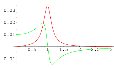
At low frequencies the phase velocity is subluminal. At frequencies the imaginary part of has an absorption peak and the phase velocity changes over to being superluminal. At high frequencies, the phase velocity approaches 1 as . It is important to emphasize that the superluminal phase velocity at high frequencies is not associated with a violation of causality since asymptotically it approaches .
5.1 The analytic structure of the integrand
When we compare our result (66) to the simple model of a dissipative medium (69), the most striking difference is the existence of singularities in the integrand. When is real, the integrand (66) has branch point singularities on the positive real axis at
| (70) |
and the integral must be properly defined in order to have a finite result. The correct procedure is to take the contour to lie just below the real axis. It is significant that these singularities arise from zeros of the fluctuation determinant (58) and have a natural interpretation in terms of zero modes, viz. non-trivial solutions of (55) with zero eigenvalue . For the special case when these zero modes are particularly simple: as in (18) and
| (71) |
The expression for is then completely determined by solving the geodesic equation
| (72) |
These solutions are therefore associated with geodesics that are arbitrarily close to that intersect at both and for at points in between. In other words, are conjugate points on the geodesic . The and zero modes are illustrated in Figure (6).
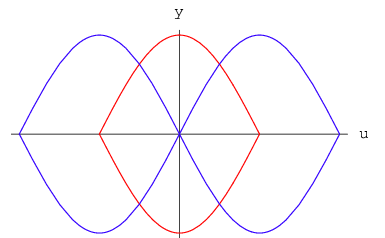
For generic the solutions are more complicated: again as in (18) while
| (73) |
and solves (72). Imposing the continuity of and the conditions (57) implies that for odd we must have
| (74) |
and so there is only a single zero mode. For even, however, there are two zero modes since there are only two conditions on the four constants:
| (75) |
Once again these solutions are formed from portions of two inequivalent geodesics which intersect at and : in other words, the points and are conjugate, however, for the conjugate points do not generally lie on . An example of the first zero mode is illustrated in Figure (7).
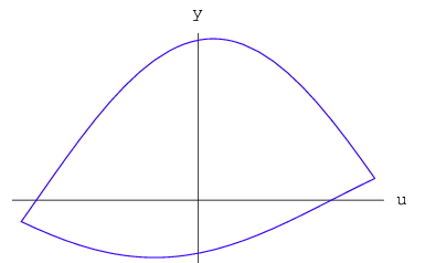
Similarly the singularities on the imaginary axis that arise when one of the is imaginary can be understood in terms of these zero modes, but with imaginary affine parameter . It is tempting to think that these solutions in imaginary affine parameter can be associated with world-line instanton solutions. These kinds of instanton in the world-line sigma model (not to be confused with instantons in the original field theory) have been discussed in the literature in the context of non-trivial electromagnetic backgrounds and can be used to describe Schwinger pair creation in that context [36, 37]. Here, we shall shortly see why this interpretation is exactly right, since the singularities on the imaginary axis determine the imaginary part of the refractive index which describes the dissipative nature of the propagation that arises from the physical process . In the world-line instanton interpretation this is described as a tunneling process.
Now that we have explained the origin of the singularities, we can continue with the analysis of (66). In order to produce a convergent integral, the Wick rotation can be performed as illustrated in Figure (8).

Once Wick rotated, the resulting integral has the form of an inverse Borel transform:
| (76) |
When is imaginary, i.e. the Type II case, there are branch point singularities on the integration contour and one has to be careful to take the contour to lie above the real axis as indicated by the prescription.
Since the integral is of the form where the function satisfies the reality condition , it follows that the imaginary part of the integral is equal to , where is a contour that comes in from below the cut, goes round the first branch point singularity and then goes to above the cut, as illustrated in Figure (9).

Hence,
| (77) |
The imaginary part of the refractive index has an interesting interpretation because it computes the probability for pair creation, . In fact the total cross-section per unit volume, or inverse mean free path, is
| (78) |
Notice that it is only non-vanishing in the Type II case when there are singularities on the real axis in the (Euclidean) plane. Earlier we pointed out that these singularities correspond to non-trivial classical loops with imaginary affine parameter. We can now identify these solutions as world-line instantons that describe the tunnelling process . The fact that they occur only when is imaginary is natural. Remember, when is imaginary the null congruence is defocusing in the direction. This suggests the following intuitive picture: after a virtual pair is produced by tunnelling, the pair then follow diverging geodesics and become real particles.
At low frequencies, the probability is dominated by the position of the first singularity at
| (79) |
in Euclidean space, corresponding to the fundamental world-line instanton which looks exactly like the red loop in Figure (6) in Euclidean time. The Euclidean action of a zero mode is simply , and for small we can use the steepest decent method to approximate the integral. The saddle-point is at and hence the leading order behaviour of (77) for small will be of the form of an essential singularity:
| (80) |
5.2 The low frequency regime
Low frequency means that . As a consequence of this, the length of the loop (18), , is much smaller than the curvature scale: . The leading order term in this limit will consequently be insensitive to the dependence of and so our result for this term is valid for all background metrics and not just ones which yield symmetric plane waves in the Penrose limit.
To calculate the expansion in , we expand the Wick rotated integrand in (76) in powers of . The first term in the expansion is independent:
| (81) |
and so there is no dispersion in this limit. Using (37), this can be written in terms of the curvature, and the Newman-Penrose scalars, as
| (82) |
for . In principle, this low frequency expression should follow from the terms in the low energy one-loop effective action of scalar QED that are quadratic in the field strength and linear in the curvature. These terms have been calculated in spinor QED [2, 18, 19] but not, to our knowledge, in scalar QED.2020 20 Even given the effective action, one must be very careful in simplifying with integration by parts because the on-shell photon wavefunction does not fall off at infinity.
It is interesting to consider the higher terms in the frequency expansion in certain particular examples. For example, for the case of a Type I conformally flat background, , the velocity eigenstates for both polarizations have
| (83) |
This series is divergent but alternating and this is correlated with the fact that it is Borel summable, with the sum being defined by the convergent integral in (76) which has no singularities on the real axis. Notice that is real to all orders in the expansion and since there are no cuts on the real axis the imaginary part vanishes, as is evident in (77).
For the Type II Ricci flat background, , one polarization is superluminal at low frequencies with
| (84) |
For the second, subluminal, polarization eigenstate,
| (85) |
The first series (84) is just the alternating version of (85). In both cases the Borel transforms have branch point singularities on the real axis and this is indicative of an imaginary part (80) which vanishes to all orders in the expansion.
5.3 The high frequency regime
In the high-frequency limit , by re-scaling and expanding , we can show that the approach 1 like :
| (86) |
where is the integral
| (87) |
Notice that the behaviour of the subleading term is softer than . For the conformally flat case with , the integral (87) can be evaluated exactly by contour integration yielding
| (88) |
for both .
For the Ricci flat Type II case (the vacuum gravitational wave), , although we cannot evaluate analytically, there is an interesting relation
| (89) |
that follows from the definition of the integrals. A numerical evaluation in this case gives
| (90) |
which implies that both polarization states are superluminal at high frequencies. Hence, must change from being greater than to less than at some intermediate frequency.
5.4 Numerical analysis
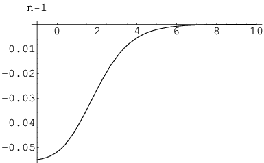
Type I: In this case, the integrand (76) is regular on the real axis and so the resulting refractive indices are real and there is no pair creation. Figure (10) shows a numerical evaluation for the conformally flat background with .
(a)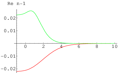 (b)
(b)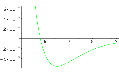
(a)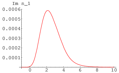 (b)
(b)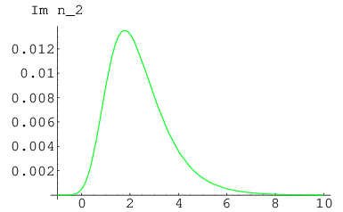
Type II: In this case, the integrand (76) has branch point singularities on the real axis. From the point of view of a numerical evaluation, it is therefore not useful to perform the Wick rotation. A useful alternative is to perform a “half” Wick rotation by rotating the contour of (66) to lie along . The resulting integral is convergent and can then be evaluated numerically. We find that the refractive indices have both a real and imaginary part, as we anticipated earlier. Figures (11) and (12) show the real and imaginary parts of for the example of a Ricci flat background with . Notice that the subluminal polarization state behaves superficially like our simple model of a dissipative medium in Figure (5).
6 Micro-Causality and the Kramers-Kronig Relation
Before we analyse our curved spacetime result, let us first consider the simple model of a dissipative medium. In that case, from (68) we see that has simple poles in the lower-half plane at (for ). Hence, is analytic in the upper-half plane and the Kramers-Kronig relation is trivially satisfied. To see this, consider for a contour along the real axis, jumping over the simple pole at , completed by the large semi-circle in the upper-half plane, illustrated in Figure (13). If is analytic in the upper-half plane, the total integral is 0 and so:
| (91) |
Taking the imaginary part, and assuming that and are real and that is an odd function, immediately yields (1). It is a simple matter to check the relation explicitly for the dissipative model (68).
(a) (b)
(b)
For curved spacetime this argument fails because there are singularities on the imaginary axis which have to be included in (91), as illustrated in Figure. (13). For example, for the conformally flat Type I case, , the singularities are poles whose residues must be included:2121 21 For more general examples, the singularities are branch points and the integration contour has to come around them from down the imaginary axis before going back to and completing the semi-circle.
| (92) |
Since in this case , and including the contribution from the poles on the imaginary axis, (92) becomes
| (93) |
where we have defined the function
| (94) |
The residue sum can be regularized by considering and taking at the end. The result is
| (95) |
which is in perfect agreement with (83) and (86). Notice that we have established this result by interchanging the order of the and integrals in which case the singularities appear as poles on the imaginary axis. However, if we perform the integral first, then the singularities become a branch cut in from 0 to in the upper half plane.
The fact that is not analytic in the upper-half plane is intimately connected with the issue of micro-causality, as we now explain. In our simple model of a dissipative medium, the Fourier transform of the susceptibility, ,
| (96) |
plays the rôle of a response function: . In the simple model, and hence is analytic in the upper-half plane and so, when , we can compute the integral by completing the contour with a semi-circle at infinity in the upper-half plane. Since there are no singularities, the integral vanishes implying : cause precedes effect. Taking the explicit Fourier transform, we have
| (97) |
In the curved spacetime case, is not analytic in the upper-half plane and so it implies that the analogue of will be non-vanishing for .
We now place this simple analysis in the context of relativistic QFT, where response functions are more properly understand in terms of (retarded) propagators. The one-loop vacuum polarization contributes to the propagator via . In a real space picture, the issue of micro-causality rests on the fact that the retarded propagator is only non-vanishing in, or on, the forward light cone.2222 22 When we talk in the following about the “light cone” we mean the geometrical null surface defined by the metric . In prosaic language, an external source can only influence the fields in the future. For instance, in the present context the real space tree-level retarded propagator is only non-vanishing on the forward light cone. However, what about the one-loop correction? Notice that we have only calculated on-shell in momentum space and this means that we do not have access to the complete one-loop real space propagator. However, we can perform the Fourier transform with respect to , which determines the propagator as a function of the null coordinate :
| (98) |
This is a retarded quantity if the integration contour is taken to avoid singularities by veering into the upper-half plane, when , and the lower half plane, when . For QFT in flat spacetime, is analytic in the upper-half plane and so when one computes the integral by completing the contour with a semi-circle at infinity in the upper-half plane. Since there are no singularities in the upper-half plane, the integral vanishes and consequently for . This is consistent with the fact that the region lies outside the forward light cone. Hence, in this case micro-causality is preserved as a consequence of analyticity in the upper-half plane in frequency space. In curved spacetime, on the contrary, is not analytic in the upper-half plane and consequently it would seem that the one-loop retarded propagator must receive contributions from the region which lies outside the forward light cone. See Figure (14).

The idea here, is that is identified with one of the lightcone momenta . When the photon is on-shell at tree level, the other component vanishes, . Now by giving a small positive imaginary part a non-analyticity in the upper-half plane would be in the region which means that the retarded propagator is non-vanishing outside the lightcone. However the loophole in this reasoning is that once the and integrals have been performed, the non-analyticities of as a function of arises as branch cuts joining to . When taken off-shell, it may be that the branch cut slips into the causally safe region . The only way to really settle this issue is to perform a calculation of the vacuum polarization with the momentum off-shell [40].2323 23 Note added: We have now completed a full off-shell calculation of the vacuum polarization tensor and find that precisely this behaviour occurs. The branch point at is shifted to with . Full details will be presented elsewhere [41].
One final point to emphasize is that in the Type II examples where the imaginary part of the refractive index is non-vanishing, it is positive as expected from the optical theorem2424 24 It is amusing to note that here we are applying the optical theorem in its original context of the refractive index from which the name of the theorem is derived. which relates it to the total cross-section per unit volume, or inverse mean free path as in (78). In this sense, spacetime acts as an ordinary dissipative medium. However, unlike the simple dissipative model where the imaginary part of the refractive index falls off as , for curved spacetime the imaginary part falls off as . This implies that the mean free path saturates to a constant .
7 Remarks on General Backgrounds
In this section, we consider some of the features of our analysis which apply in more general non-symmetric plane wave backgrounds when does not take the special form (35). For the moment, we shall assume that the Penrose limit is non-trivial, i.e. not flat space. Our purpose is to highlight how the resulting behaviour of the refractive index depends to a large extent on the properties of the null congruence.
At the beginning of Section 5, we found that the analytic structure of the integrand (66) – more precisely the positions of the singularities – could be traced to the existence of zero modes of the fluctuation equations. In the general case, the equation for these zero modes is
| (99) |
Considering the solutions of these 2nd order equations in the two regions and , and including and , there are generically nine unknowns to be fixed, up to overall scaling of the solution. At and there are a total of eight boundary conditions on and , with the constraint providing a ninth condition. In general, we therefore expect solutions to exist only for particular values of . This is exactly what we found for the symmetric case where the special values of are given in (70). Although, for even we found two zero modes rather than the one expected.
As we have seen, the existence of the zero modes is related to the behaviour of the null congruence. This can be made more concrete by looking at the special case when (which is, in any case, picked out by the saddle-point method described above). In this case, by symmetry we expect a solution of the form that we found in the symmetric plane wave case, (71), but where the transverse geodesic deviation vector satisfies the equation for a Jacobi field along the geodesic :
| (100) |
subject to the boundary conditions . Because of the latter, the source terms vanish and so the derivatives must be continuous at and , a fact that follows directly from the ansatz (71). In addition, the constraint is automatically satisfied and the Lagrange multiplier vanishes. The classical solution is then , (with a slight abuse of notation) and satisfies its own geodesic equation. Since (100) is a second order linear equation there will in general be solutions only for particular values of . Since vanishes at , at least when the special values of are real, these points are precisely conjugate points along . Hence, the existence of zero modes (for real values of ) is tied directly to the existence of conjugate points. Notice, however, that the special values of for which zero modes exist are not necessarily real. This is exactly what happens in the Type II examples, where the singularities corresponding to world-line instantons have imaginary .
The zero modes dictate the analytic structure of the integral which in turn determines the nature of the physics. In particular, the singularities along the real axis play a prominent rôle because, as we have seen, they are responsible for the non-trivial analytic structure of . Moreover, as we have argued above, zero modes for real correspond directly to the existence of conjugate points along . But the existence of these conjugate points, as explained in Section 3, is generic. Therefore we are led to the following conclusion:
Conclusion: violations of analyticity and the Kramers-Kronig relation are generic and can be traced to the focusing nature of null geodesics and the existence of conjugate points implied by the null energy condition.
As already mentioned, the Penrose limit is ideally suited to the analysis of photon propagation in arbitrary background spacetimes. Many of the characteristic features of superluminal low-frequency propagation previously found in specific examples, including Schwarzschild, Reissner-Nordström and Kerr black holes [2, 16, 32] as well as gravitational waves [2, 17], can be seen directly in the Penrose limit. For example, a maximally symmetric spacetime such as de Sitter has vanishing and and the low-frequency phase velocity receives no correction from vacuum polarization. Using our formalism, we see immediately that at leading order in this result holds for all frequencies since the Penrose limit of a maximally symmetric spacetime is flat [24].
In Schwarzschild spacetime, we have previously found that while a photon following a general null geodesic may experience a superluminal shift in , the effect vanishes for purely radial geodesics. (In fact, this remains true for photons following principal null geodesics [31] for any Petrov type D spacetime such as Schwarzschild or Kerr, again due to the vanishing of the corresponding and .) This is clear in our formalism. The Penrose plane wave limit for the Schwarzschild metric is, in Brinkmann coordinates,
| (101) |
where specifies the angular momentum and is given by the solution of the geodesic equation. We see immediately that for radial trajectories the Penrose limit is flat and so, at least at , the phase velocity remains equal to for all frequencies, not just in the low-frequency limit. Clearly, in such cases where the Penrose limit is flat, the expansion (32) gives a systematic way to go beyond leading order in . An interesting feature is the existence of a “peeling theorem”[24], whereby successive orders in the Penrose expansion involve the curvatures .
This gives a first glance at the power of the Penrose plane wave geometry combined with the world-line sigma model approach. Moreover, other general features of null congruences will play an important rôle. For example, we have been implicitly assuming that the geodesics are complete so that the affine parameter varies from to . However, there are spacetimes where certain null geodesics are incomplete and the affine parameter has a finite limiting value. This usually signals the existence of a spacetime singularity, as for example in the case of Schwarzschild orbits for less than a critical value, where the Penrose limit becomes singular [24]. Clearly, this can affect the zero modes in the sigma model and therefore the singularities and asymptotic behaviour of the refractive index. The rôle of horizons in relation to the Penrose limit also deserves investigation. All of these issues will be considered in detail elsewhere.
8 Conclusions
In this paper, we have for the first time evaluated the non-perturbative frequency dependence of the vacuum polarization for QED in curved spacetime and determined the corresponding refractive index for photon propagation. In so doing, we have resolved the outstanding problem in “quantum gravitational optics” [4, 5], viz. how to reconcile the prediction of a superluminal phase velocity at low frequency with causality. Remarkably, the resolution involves the violation of analyticity calling into question micro-causality in curved spacetime.
These results have been achieved by combining two powerful techniques: (i) the world-line sigma model, which enables the non-perturbative frequency dependence of the vacuum polarization to be evaluated by a saddle-point expansion around a geometrically motivated classical solution, and (ii) the Penrose plane wave limit, which encodes the relevant tidal effects of spacetime in the neighbourhood of the original null geodesic traced by the photon.
The form of the refractive index reflects the nature of the background spacetime. We identify two classes. In Type I backgrounds, which include conformally flat spacetimes,2525 25 Note that the Penrose limit of a conformally flat spacetime is also conformally flat. Similarly for Ricci flat, and also locally symmetric, spacetimes [24]. both photon polarizations are superluminal at low frequencies, but the phase velocity approaches at high frequency. The imaginary part of the refractive index vanishes. In Type II backgrounds, which include Ricci flat spacetimes, photon propagation may display birefringence with one superluminal and one subluminal polarization at low frequency. In both cases, however, the high frequency phase velocity is . The refractive index develops an imaginary part, indicating a non-zero probability for pair creation, . Since the high-frequency limit of the phase velocity is identified with the wavefront velocity , which is the “speed of light” relevant for causality, we see explicitly how superluminal propagation in the low-frequency theory is compatible with causality.
Although these results were obtained using the Penrose limit in locally symmetric spacetimes, they are expected to be generally true. The reason is that the analytic properties of the refractive index can be related in the world-line sigma model formalism to general results in the theory of null congruences. In particular, the distinction between Type I and Type II spacetimes is whether the null geodesics in the congruence focus in both transverse directions (Type I), or focus in one and defocus in the other (Type II). The result that at least one direction is focusing is a consequence of the null energy condition. The presence of a focusing direction in the congruence then implies the existence of conjugate points, which leads to the existence of zero modes and ultimately yields poles in the refractive index in the upper-half complex plane, violating the analyticity assumptions used to derive the Kramers-Kronig dispersion relation. The violation of this dispersion relation in turn allows and removes the apparent paradox of having a superluminal phase velocity while the wavefront velocity .
This is potentially the most far-reaching conclusion of this paper. The null energy condition and the general relativistic theory of null congruences necessarily imply a non-analyticity of the refractive index, although the full implications of this for micro-causality and the other axioms of S-matrix theory will only follow from an off-shell extension of the calculation.
The loss of analyticity in , or more generally in forward scattering amplitudes, also has important implications for the idea that constraints may be placed on the parameters of a low-energy effective field theory by the requirement that it admits a consistent UV completion [5, 38, 39]. These constraints are typically derived either by requiring the absence of superluminal effects in the low-energy theory or assuming analyticity in dispersion relations involving forward scattering amplitudes. While these remain valid in flat spacetime, we have shown that they are not applicable to fundamental UV theories involving gravity, including string theory.
The full implications of the calculation of the refractive index and the issues of causality and micro-causality remain to be explored, especially in relation to horizons and singularities. The significance of the UV-IR mixing whereby the high-frequency limit probes the global properties of the null geodesic congruence also deserves to be better understood. What is clear, however, is that the results described here will have a significant impact on our understanding of quantum field theories involving gravity.
We would like to thank Asad Naqvi for many useful conversations and Sergei Dubovsky, Alberto Nicolis, Enrico Trincherini and Giovanni Villadoro for pointing out the necessity of working off-shell in order to completely settle the question of micro-causality. TJH would also like to thank Massimo Porrati for a helpful discussions and Fiorenzo Bastianelli for explaining some details of his work on the world-line formalism. This work was supported in part by PPARC grant PP/D507407/1.
Appendix A: Power Counting
In this Appendix, we prove in an alternative way one of the key results of this paper: that each loop in the world-line QFT comes with a power of and so loops are suppressed in the limit of weak curvature . In order to assess the behaviour of a given graph in perturbation theory, it is useful to re-scale and then and so that the world-line action can be split as
| (102) |
where a typical term in arises from expanding the metric around flat space at the point ; schematically,
| (103) |
where denotes powers of the Riemann tensor and its derivatives of mass dimensions . The vertex behaves as and has legs. In addition, we have the exponential factors which we can view as additional vertices of the form
| (104) |
Consider such a graph with external legs, internal legs and vertices. If the graphs consists of vertices of the form (103) and vertices of the form (104), then
| (105) |
The graph behaves as
| (106) |
Now we use the topological identity, , where is the number of loops, to equate this to
| (107) |
So each loop brings a factor of . For example, the partition function has and since the tree-level contribution is the classical action for the saddle point which vanishes, the leading order term comes from one loop and is an arbitrary function of . The expansion around the classical saddle-point solution sums up all the one-loop graphs with arbitrary insertions. The leading order contribution to the Green’s function piece, which has , comes from tree level. Once again, the expansion around the classical saddle-point solution sums up all these tree graphs with arbitrary insertions.
References
- [1]
- [2] I. T. Drummond and S. J. Hathrell, Phys. Rev. D 22 (1980) 343.
- [3] G. M. Shore, “Causality and Superluminal Light”, in ‘Time and Matter’, Proceedings of the International Colloquium on the Science of Time, ed. I. Bigi and M. Faessler, World Scientific, Singapore, 2006. [arXiv:gr-qc/0302116].
- [4] G. M. Shore, Contemp. Phys. 44 (2003) 503 [arXiv:gr-qc/0304059].
- [5] G. M. Shore, arXiv:hep-th/0701185.
- [6] M. A. Leontovich, in L.I. Mandelshtam, “Lectures in Optics, Relativity and Quantum Mechanics”, Nauka, Moscow, 1972 (in Russian).
- [7] S. Weinberg, “The Quantum Theory of Fields”, Vol I, Cambridge University Press, 1996.
- [8] T.J. Hollowood and G.M. Shore, “Causality and Micro-Causality in Curved Spacetime,” arXiv:0707.2302 [hep-th]
- [9] S. W. Hawking and G. F. R. Ellis, “The Large Scale Structure of Spacetime”, Cambridge University Press, 1973.
- [10] S. Liberati, S. Sonego and M. Visser, Annals Phys. 298 (2002) 167 [arXiv:gr-qc/0107091].
- [11] P. B. Gilkey, J. Diff. Geom. 10 (1975) 601.
- [12] A. O. Barvinsky, Yu. V. Gusev, G. A. Vilkovisky and V. V. Zhytnikov, Print-93-0274 (Manitoba), 1993.
- [13] A .O. Barvinsky, Yu. V. Gusev, G. A. Vilkovisky and V. V. Zhytnikov, J. Math. Phys. 35 (1994) 3525; J. Math. Phys. 35 (1994) 3543; Nucl. Phys. B 439 (1995) 561.
- [14] I. G. Avramidi, Rev. Math. Phys. 11 (1999) 947 [arXiv:hep-th/9704166].
- [15] A. O. Barvinsky, Yu. V. Gusev, V. F. Mukhanov and D. V. Nesterov, Phys. Rev. D 68 (2003) 105003 [arXiv:hep-th/0306052].
- [16] R. D. Daniels and G. M. Shore, Nucl. Phys. B 425, 634 (1994) [arXiv:hep-th/9310114]; Phys. Lett. B 367, 75 (1996) [arXiv:gr-qc/9508048].
- [17] G. M. Shore, Nucl. Phys. B 605 (2001) 455 [arXiv:gr-qc/0012063].
- [18] G. M. Shore, Nucl. Phys. B 646 (2002) 281 [arXiv:gr-qc/0205042].
- [19] G. M. Shore, Nucl. Phys. B 633 (2002) 271 [arXiv:gr-qc/0203034].
- [20] R. P. Feynman, Phys. Rev. 80 (1950) 440.
- [21] J. S. Schwinger, Phys. Rev. 82 (1951) 914.
- [22] C. Schubert, Phys. Rept. 355 (2001) 73 [arXiv:hep-th/0101036].
- [23] R. Penrose, “Any space-time has a plane wave as a limit”, in: Differential geometry and relativity, Reidel and Dordrecht (1976), 271-275.
- [24] M. Blau, “Plane waves and Penrose limits”, Lectures given at the 2004 Saalburg/Wolfersdorf Summer School, http://www.unine.ch/phys/string/Lecturenotes.html
- [25] M. Blau, D. Frank and S. Weiss, Class. Quant. Grav. 23 (2006) 3993 [arXiv:hep-th/0603109].
- [26] F. Bastianelli and A. Zirotti, Nucl. Phys. B 642 (2002) 372 [arXiv:hep-th/0205182].
- [27] F. Bastianelli, O. Corradini and A. Zirotti, JHEP 0401 (2004) 023 [arXiv:hep-th/0312064].
- [28] F. Bastianelli, arXiv:hep-th/0508205.
- [29] H. Kleinert and A. Chervyakov, Phys. Lett. A 308 (2003) 85 [arXiv:quant-ph/0204067].
- [30] H. Kleinert and A. Chervyakov, Phys. Lett. A 299 (2002) 319 [arXiv:quant-ph/0206022].
- [31] S. Chandresekhar, “The Mathematical Theory of Black Holes”, Clarendon, Oxford, 1985.
- [32] G. M. Shore, Nucl. Phys. B 460 (1996) 379 [arXiv:gr-qc/9504041].
- [33] G. W. Gibbons and C. A. R. Herdeiro, Phys. Rev. D 63 (2001) 064006 [arXiv:hep-th/0008052].
- [34] R. M. Wald, “General Relativity,” Chicago University Press, 1984.
- [35] J. D. Jackson, “Classical Electrodynamics” 2nd Edition, Wiley 1975.
- [36] I. K. Affleck, O. Alvarez and N. S. Manton, Nucl. Phys. B 197 (1982) 509.
- [37] G. V. Dunne and C. Schubert, Phys. Rev. D 72 (2005) 105004 [arXiv:hep-th/0507174].
- [38] A. Adams, N. Arkani-Hamed, S. Dubovsky, A. Nicolis and R. Rattazzi, JHEP 0610 (2006) 014 [arXiv:hep-th/0602178].
- [39] J. Distler, B. Grinstein, R. A. Porto and I. Z. Rothstein, Phys. Rev. Lett. 98 (2007) 041601 [arXiv:hep-ph/0604255].
- [40] S. Dubovsky, A. Nicolis, E. Trincherini and G. Villadoro, “Microcausality in Curved Space-Time,” arXiv:0709.1483 [hep-th].
- [41] T.J. Hollowood and G.M. Shore, in preparation.
- [42]