Four-Loop Collinear Anomalous Dimension in ${\mathcal{N}}=4$ Yang-Mills Theory

Gluon scattering amplitudes in QCD and supersymmetric gauge theories are notoriously difficult to compute, yet possess remarkably simple hidden structure. We expect the greatest simplicity in the maximally supersymmetric ${\cal N}=4$ Yang–Mills theory, where planar $L$-loop amplitudes are believed to satisfy iterative relations Anastasiou:2003kj; Magnea:1990zb; Catani:1998bh; Sterman:2002qn; Cachazo:2006tj; Bern:2006vw; Bern:2005iz in $L$. These relations allow the complete, planar all-loop $n$-particle MHV amplitude ${\mathcal{A}}$ to be written in an exponential form due to Bern, Dixon and Smirnov Bern:2005iz. Their ansatz for the $n=4$ particle amplitude is

where $\lambda=g_{\rm YM}^{2}N$ is the ’t Hooft coupling, $s$ and $t$ are the usual four-particle Mandelstam invariants, and the infrared divergences are encoded in the prefactors ${\cal A}_{\rm div}$. In dimensional regularization to $D=4-2\epsilon$ the divergences take the form

in terms of an IR cutoff scale $\mu$ (required on dimensional grounds) and two functions $f^{(-2)}(\lambda)$ and $g^{(-1)}(\lambda)$ which respectively are related to the $f(\lambda)$ appearing in (1) and to a second function called $g(\lambda)$ according to

The three functions $f(\lambda)$, $g(\lambda)$ and $c(\lambda)$ are universal; the same functions appear in the exponential ansatz for any planar $n$-particle MHV amplitude Bern:2005iz.

The function $f(\lambda)$ is well-known from another role: it is the cusp anomalous dimension, which also governs the scaling of twist-two operators in the limit of large spin $S$ Korchemsky:1988si; Korchemsky:1992xv; Gubser:2002tv; Kruczenski:2002fb,

At weak coupling it has been computed through four loops Moch:2004pa; Vogt:2004mw; Kotikov:2004er; Bern:2006ew; Cachazo:2006az,

with $r=-2.00002(3)$ (the quantity in parentheses denotes the current best numerical uncertainty in the last digit), while AdS/CFT calculations Gubser:2002tv; Frolov:2002av indicate the strong coupling behavior

The recently proposed dressing phase Beisert:2006ib; Beisert:2007hz for the asymptotic S-matrix Beisert:2004hm; Arutyunov:2004vx; Staudacher:2004tk; Beisert:2005fw; Beisert:2005tm; Eden:2006rx of the spin chain description of planar ${\cal N}=4$ Yang-Mills implies that at finite $\lambda$, $f(\lambda)$ satisfies a certain integral equation Beisert:2006ez whose solution is compatible with the limits (7), (9) Benna:2006nd; Alday:2007qf; Casteill:2007ct and moreover predicts that $r=-2$ in (7).

Much less is known about the second function $g(\lambda)$ which governs the subleading infrared divergence and may be called the “collinear” anomalous dimension Korchemsky:1994is. Perturbative calculations through three loops Bern:2005iz have established that

and the purpose of this note is to report a numerical calculation of the four-loop coefficient

It is an important outstanding problem to relate $g(\lambda)$ to more familiar observables which could perhaps be computed using integrability techniques. In particular it would be interesting to derive an integral equation satisfied by $g(\lambda)$.

An important step forward was recently taken by Alday and Maldacena Alday:2007hr, who gave a prescription for computing gluon amplitudes at strong coupling using AdS/CFT and found perfect agreement with the ansatz (1). A consequence of their calculation is the prediction

for the leading strong-coupling behavior of $g(\lambda)$. It is important to mention that while $f(\lambda)$ is independent of the IR renormalization scale, the same is not true for $g(\lambda)$. Rescaling $\mu$ to $k\mu$ sends $g(\lambda)$ to $g(\lambda)+2\log(k)f(\lambda)$.

In section II we review our calculational method, which is the same as the one used in Cachazo:2006az to calculate $f^{(4)}$ to very high accuracy. In section III we explore the connection between the weak- and strong-coupling behavior of $g(\lambda)$. First we use the Alday-Maldacena result (13), together with the known data (11) through three loops, to build an interpolating function and make a ‘prediction’ for $g^{(4)}$. Remarkably our result (12) is within $7\%$ of this predicted value. Finally we use all currently available data on $g(\lambda)$ to construct a Padé approximant which represents our best guess for the function’s behavior at finite $\lambda$.

To compute $g^{(4)}$ we apply the method of obstructions developed in Cachazo:2006mq; Cachazo:2006az. We begin with the four-loop iterative structure encoded in (1), which in dimensional regularization takes the form Bern:2005iz

where $M^{(L)}(\epsilon)$ is the ratio of the $L$-loop amplitude to the tree amplitude and $f_{0}^{(4)}$, $f_{1}^{(4)}$ are two numbers. According to Bern:2005iz, whose conventions we follow except as noted below, these are related to the four-loop coefficients $f^{(4)}$ and $g^{(4)}$ in $f(\lambda)$ and $g(\lambda)$ by

The factor of $1/2^{4}$ arises here at four loops because the expansion parameter used by Bern:2005iz differs by a factor of $2$ from that of Alday:2007hr which we use in (7) and (11).

Each of the five terms on the left-hand side of (14) is separately an extremely complicated function of the ratio $x=t/s$ with singular behavior starting at ${\cal O}(1/\epsilon^{8})$. It is therefore rather remarkable that the five terms conspire to add up to such a simple object involving only two free constants Magnea:1990zb; Catani:1998bh; Sterman:2002qn. The leading singularity of $M^{(1)}(4\epsilon)$ on the right-hand side is ${\cal O}(1/\epsilon^{2})$, so we can determine $f^{(4)}_{1}$ by reading off the coefficient of the $1/\epsilon$ pole on both sides of (14).

The idea behind the method of obstructions, explained in detail in Cachazo:2006az, is that we do not need to fully compute all of the $M^{(L)}(\epsilon)$. Rather, it is sufficient to compute what are in some sense the ‘constant pieces’, since the $x$-dependent pieces are guaranteed to cancel each other out on the left-hand side of (14). This idea is made precise by writing each amplitude as a Mellin transform, in the form

for some $F(y,\epsilon)$. It turns out that $f_{1}^{(4)}$ multiplies $\delta(y)$ in Mellin space, so in order to isolate this term it is sufficient to read off just the coefficient of $\delta(y)$ on both sides of (14), throwing away the rest. We call terms proportional to $\delta$-functions obstructions. The utility of this method benefits significantly from the fact that we can work directly in Mellin space, where it is relatively easy to construct explicit formulas for Feynman integrals Smirnov:1999gc; Tausk:1999vh.

It was further shown in Cachazo:2006az that obstructions obey a product algebra structure, meaning that the obstruction in any product of amplitudes is given by the product of their obstructions. This statement is obvious in $y$-space where it hinges on the simple fact that $\delta(y)$ convolved with itself is again $\delta(y)$. Consequently we can calculate the obstruction $P^{(L)}(\epsilon)$ in each $M^{(L)}(\epsilon)$ separately and then insert those results into the polynomial in (14).

The $L=1,2,3,4$ loop amplitudes we require may be expressed in terms of the 12 scalar Feynman diagrams depicted in Fig. 1 Green:1982sw; Bern:1997nh; Bern:2005iz; Bern:2006ew. The reader may find all necessary details in Bern:2005iz; Bern:2006ew. Our convention is that each loop momentum integral comes with a factor

The standard convention includes only the factor in brackets. The additional factor $(-s)^{\epsilon/2}(-t)^{\epsilon/2}$ renders all amplitudes dimensionless (when the appropriate numerator factors are included), but it does not alter the form of (14) since each term in that equation has a common factor $(-s)^{-2\epsilon}(-t)^{-2\epsilon}$. The factor of $-1/2$ in front here eliminates the need for a factor of $(-1/2)^{L}$ in (18) below.

We have computed the obstructions in the 12 separate integrals through the first eight orders in $\epsilon$ and present the results in equation (28) at the end of the paper. The calculation was performed using the algorithm explained in Cachazo:2006az based on Czakon’s MB program Czakon:2005rk. Numerical integrations were performed using CUBA’s Cuhre algorithm Hahn:2004fe, and the digit in parentheses denotes the reported uncertainty in the final digit.

An exact formula for ${\mathcal{I}}^{(1)}(\epsilon)$ was given in Cachazo:2006az, as were the first seven terms in the two- and three-loop amplitudes (though here we indicate separately the contributions from the two three-loop integrals). No significant effort was spent on attempting to improve the numerical accuracy of the ${\cal O}(1/\epsilon^{3})$ and ${\cal O}(1/\epsilon^{2})$ terms in the individual four-loop integrals because these values play no role in this paper.

To find the full obstruction $P^{(L)}$ in the $L$-loop amplitude we add together the contributions from the individual integrals according to Green:1982sw; Bern:1997nh; Bern:2005iz; Bern:2006ew

Plugging the resulting expressions for $P^{(L)}$ into (14) in place of $M^{(L)}$ and using the relation (15) leads to the advertised value (12).

As mentioned above, string theory provides predictions for how $f(\lambda)$ and $g(\lambda)$ behave at strong coupling. It is therefore tempting to try to make a connection between the weak and strong coupling regimes. An approximation scheme that has been very successful for $f(\lambda)$ is the following. If $n+1$ orders of the expansion around $\lambda=0$ are known, then one constructs an approximating function $\hat{f}(\lambda)$ as an appropriate solution to the polynomial equation Kotikov:2003fb

where the coefficients $c_{r}$ are determined by imposing that $\hat{f}(\lambda)$ agree with $f(\lambda)$ through ${\cal O}(\lambda^{n+1})$.

The form of (23) incorporates a strong coupling expansion for $\hat{f}(\lambda)$ in the parameter $4\pi/\sqrt{\lambda}$ with leading term $\alpha\sqrt{\lambda}/4\pi$ where $\alpha^{2n}=1/c_{2n}$.

Using the expansion of $f(\lambda)$ up to four loops one finds an approximating function $\hat{f}(\lambda)$ that agrees, within a few percent, with the string theory strong coupling prediction and with the BES ansatz Beisert:2006ez for all positive values of the coupling.

The success of this approximation scheme makes its application to $g(\lambda)$ a natural thing to attempt. However, since $g(\lambda)$ is negative for small $\lambda$ but becomes positive at strong coupling, it must have at least one zero for $\lambda>0$. Clearly, any approximating function of the form (23) (with an appropriate modification because $g(\lambda)$ only starts at two loops)

leads to a $\hat{g}(\lambda)$ that cannot possibly have a zero for $\lambda\neq 0$ and hence a contradiction. One way to find a consistent approximating function was introduced in Alday:2007hr. The idea is to perform a change of the IR renormalization scale $\mu\to\exp(\xi/2)\mu$. Then, as discussed above, $g(\lambda)\to g(\lambda)+\xi f(\lambda)$. The new function $\tilde{g}(\lambda,\xi)=g(\lambda)+\xi f(\lambda)$ can now be approximated by using (23) for any $\xi>0$.

Consider the approximation (23) for $\hat{\tilde{g}}(\lambda,\xi)$ with $n=2$,

This equation depends on four parameters, namely, $c_{2},c_{3},c_{4}$ and $\xi$. Imposing that the approximating function $\hat{\tilde{g}}(\lambda,\xi)$ agrees with ${\tilde{g}}(\lambda,\xi)$ through ${\cal O}(\lambda^{3})$ determines the three coefficients $c_{2},c_{3},c_{4}$ in terms of $\xi$. In Alday:2007hr the resulting approximating function was extrapolated to strong coupling and compared to the string theory prediction for a range of $\xi$. At the special value $\xi=\frac{1}{2}\log 2$, for example, the approximation gives $\hat{\tilde{g}}(\lambda)=1.37\sqrt{\lambda}/4\pi$ compared to the string theory prediction $\tilde{g}(\lambda)=2\sqrt{\lambda}/4\pi$.

Here we would like to use the results of Alday and Maldacena to make a prediction for $g^{(4)}$ to compare our result (12) to. Imposing that $\hat{\tilde{g}}$ agrees with the string theory prediction at strong coupling fixes the parameter $\xi\approx 0.73679$. Then all four parameters $c_{2},c_{3},c_{4}$ and $\xi$ are completely fixed and we can expand the resulting $\hat{\tilde{g}}$ in $\lambda$ to ${\cal O}(\lambda^{4})$ to find the predicted value $g^{(4)}\approx-1336.9$. Remarkably our result (12) is only $7\%$ away from this value. We interpret this as good evidence for the string theory strong coupling prediction of Alday and Maldacena Alday:2007hr.

Finally we present also a more conventional Padé approximant for $g(\lambda)$ based upon all currently available data. Here we follow the approach described in Bern:2006ew where a $[3/2]$ Padé approximant in terms of the auxiliary variable $u=\sqrt{1+\lambda/\pi^{2}}$ was considered for $f(\lambda)$. Specifically we consider the ansatz

with four parameters $N_{0},N_{1},D_{1},D_{2}$. The choice $u=\sqrt{1+\lambda/\pi^{2}}$ was motivated by evidence that $f(\lambda)$ should have a branch point at $\lambda=-\pi^{2}$. It seems reasonable to guess that the same might be true for $g(\lambda)$, though we have no direct evidence for this guess.

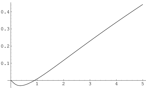
The four parameters in (26) can be uniquely determined by fitting to all available data—the perturbative expansion through four loops as well as the strong-coupling limit (13). The resulting approximant, displayed in Fig. 2, may be considered our best candidate picture of $g(\lambda)$ at the moment. Note that it is minimal in the sense that $G(\lambda)$ was designed to have a single zero along the positive real axis, whereas the true $g(\lambda)$ could potentially have any odd number of zeros. Curiously, the zero lies very close to $\lambda/16\pi^{2}=1$, although it is impossible to conclude based on the limited available data whether or not this is just a coincidence.

References

- (1) C. Anastasiou, Z. Bern, L. J. Dixon and D. A. Kosower, “Planar amplitudes in maximally supersymmetric Yang-Mills theory,” Phys. Rev. Lett. 91, 251602 (2003) hep-th/0309040.
- (2) L. Magnea and G. Sterman, “Analytic continuation of the Sudakov form-factor in QCD,” Phys. Rev. D 42 (1990) 4222.
- (3) S. Catani, “The singular behaviour of QCD amplitudes at two-loop order,” Phys. Lett. B 427, 161 (1998) hep-ph/9802439.
- (4) G. Sterman and M. E. Tejeda-Yeomans, “Multi-loop amplitudes and resummation,” Phys. Lett. B 552 (2003) 48 hep-ph/0210130.
- (5) Z. Bern, L. J. Dixon and V. A. Smirnov, “Iteration of planar amplitudes in maximally supersymmetric Yang-Mills theory at three loops and beyond,” Phys. Rev. D 72, 085001 (2005) hep-th/0505205.
- (6) F. Cachazo, M. Spradlin and A. Volovich, “Iterative structure within the five-particle two-loop amplitude,” Phys. Rev. D 74, 045020 (2006) hep-th/0602228.
- (7) Z. Bern, M. Czakon, D. A. Kosower, R. Roiban and V. A. Smirnov, “Two-loop iteration of five-point super-Yang-Mills amplitudes,” Phys. Rev. Lett. 97, 181601 (2006) hep-th/0604074.
- (8) G. P. Korchemsky, “Asymptotics of the Altarelli-Parisi-Lipatov Evolution Kernels of Parton Distributions,” Mod. Phys. Lett. A 4, 1257 (1989).
- (9) G. P. Korchemsky and G. Marchesini, “Structure function for large and renormalization of Wilson loop,” Nucl. Phys. B 406, 225 (1993) hep-ph/9210281.
- (10) S. S. Gubser, I. R. Klebanov and A. M. Polyakov, “A semi-classical limit of the gauge/string correspondence,” Nucl. Phys. B 636, 99 (2002) hep-th/0204051.
- (11) M. Kruczenski, “A note on twist two operators in SYM and Wilson loops in Minkowski signature,” JHEP 0212, 024 (2002) hep-th/0210115.
- (12) S. Moch, J. A. M. Vermaseren and A. Vogt, “The three-loop splitting functions in QCD: The non-singlet case,” Nucl. Phys. B 688 (2004) 101 hep-ph/0403192.
- (13) A. Vogt, S. Moch and J. A. M. Vermaseren, “The three-loop splitting functions in QCD: The singlet case,” Nucl. Phys. B 691 (2004) 129 hep-ph/0404111.
- (14) A. V. Kotikov, L. N. Lipatov, A. I. Onishchenko and V. N. Velizhanin, “Three-loop universal anomalous dimension of the Wilson operators in SUSY Yang-Mills model,” Phys. Lett. B 595, 521 (2004) [Erratum-ibid. B 632, 754 (2006)] hep-th/0404092.
- (15) Z. Bern, M. Czakon, L. J. Dixon, D. A. Kosower and V. A. Smirnov, “The Four-Loop Planar Amplitude and Cusp Anomalous Dimension in Maximally Supersymmetric Yang-Mills Theory,” Phys. Rev. D 75, 085010 (2007) hep-th/0610248.
- (16) F. Cachazo, M. Spradlin and A. Volovich, “Four-Loop Cusp Anomalous Dimension From Obstructions,” Phys. Rev. D 75, 105011 (2007) hep-th/0612309.
- (17) S. Frolov and A. A. Tseytlin, “Semiclassical quantization of rotating superstring in ,” JHEP 0206, 007 (2002) hep-th/0204226.
- (18) N. Beisert, R. Hernandez and E. Lopez, “A crossing-symmetric phase for strings,” JHEP 0611, 070 (2006) hep-th/0609044.
- (19) N. Beisert, T. McLoughlin and R. Roiban, “The Four-Loop Dressing Phase of SYM,” arXiv:0705.0321 [hep-th].
- (20) N. Beisert, V. Dippel and M. Staudacher, “A novel long range spin chain and planar super Yang-Mills,” JHEP 0407, 075 (2004) hep-th/0405001.
- (21) G. Arutyunov, S. Frolov and M. Staudacher, “Bethe ansatz for quantum strings,” JHEP 0410, 016 (2004) hep-th/0406256.
- (22) M. Staudacher, “The factorized S-matrix of CFT/AdS,” JHEP 0505, 054 (2005) hep-th/0412188.
- (23) N. Beisert and M. Staudacher, “Long-range Bethe ansaetze for gauge theory and strings,” Nucl. Phys. B 727, 1 (2005) [arXiv:hep-th/0504190].
- (24) N. Beisert, “The su() dynamic S-matrix,” hep-th/0511082.
- (25) B. Eden and M. Staudacher, “Integrability and transcendentality,” J. Stat. Mech. 0611, P014 (2006) hep-th/0603157.
- (26) N. Beisert, B. Eden and M. Staudacher, “Transcendentality and crossing,” J. Stat. Mech. 0701, P021 (2007) hep-th/0610251.
- (27) M. K. Benna, S. Benvenuti, I. R. Klebanov and A. Scardicchio, “A test of the AdS/CFT correspondence using high-spin operators,” Phys. Rev. Lett. 98, 131603 (2007) hep-th/0611135.
- (28) L. F. Alday, G. Arutyunov, M. K. Benna, B. Eden and I. R. Klebanov, “On the strong coupling scaling dimension of high spin operators,” JHEP 0704, 082 (2007) hep-th/0702028.
- (29) P. Y. Casteill and C. Kristjansen, “The Strong Coupling Limit of the Scaling Function from the Quantum String Bethe Ansatz,” arXiv:0705.0890 [hep-th].
- (30) G. P. Korchemsky and G. Sterman, “Nonperturbative corrections in resummed cross-sections,” Nucl. Phys. B 437, 415 (1995) hep-ph/9411211.
- (31) L. F. Alday and J. Maldacena, “Gluon scattering amplitudes at strong coupling,” arXiv:0705.0303 [hep-th].
- (32) F. Cachazo, M. Spradlin and A. Volovich, “Hidden beauty in multiloop amplitudes,” JHEP 0607, 007 (2006) hep-th/0601031.
- (33) V. A. Smirnov, “Analytical result for dimensionally regularized massless on-shell double box,” Phys. Lett. B 460, 397 (1999) hep-ph/9905323.
- (34) J. B. Tausk, “Non-planar massless two-loop Feynman diagrams with four on-shell legs,” Phys. Lett. B 469, 225 (1999) hep-ph/9909506.
- (35) M. B. Green, J. H. Schwarz and L. Brink, “ Yang-Mills And Supergravity As Limits Of String Theories,” Nucl. Phys. B 198, 474 (1982).
- (36) Z. Bern, J. S. Rozowsky and B. Yan, “Two-loop four-gluon amplitudes in super-Yang-Mills,” Phys. Lett. B 401, 273 (1997) hep-ph/9702424.
- (37) M. Czakon, “Automatized analytic continuation of Mellin-Barnes integrals,” Comput. Phys. Commun. 175, 559 (2006) hep-ph/0511200.
- (38) T. Hahn, “CUBA: A library for multidimensional numerical integration,” Comput. Phys. Commun. 168, 78 (2005) hep-ph/0404043.
- (39) A. V. Kotikov, L. N. Lipatov and V. N. Velizhanin, “Anomalous dimensions of Wilson operators in SYM theory,” Phys. Lett. B 557, 114 (2003) hep-ph/0301021.