Understanding the Properties of the BitTorrent Overlay
Abstract
In this paper, we conduct extensive simulations to understand the properties of the overlay generated by BitTorrent. We start by analyzing how the overlay properties impact the efficiency of BitTorrent. We focus on the average peer set size (i.e., average number of neighbors), the time for a peer to reach its maximum peer set size, and the diameter of the overlay. In particular, we show that the later a peer arrives in a torrent, the longer it takes to reach its maximum peer set size. Then, we evaluate the impact of the maximum peer set size, the maximum number of outgoing connections per peer, and the number of NATed peers on the overlay properties. We show that BitTorrent generates a robust overlay, but that this overlay is not a random graph. In particular, the connectivity of a peer to its neighbors depends on its arriving order in the torrent. We also show that a large number of NATed peers significantly compromise the robustness of the overlay to attacks. Finally, we evaluate the impact of peer exchange on the overlay properties, and we show that it generates a chain-like overlay with a large diameter, which will adversely impact the efficiency of large torrents.
I Introduction
Recently, Peer-to-Peer (P2P) networks have emerged as an attractive architecture for content sharing over the Internet. By leveraging the available resources at the peers, P2P networks have the potential to scale to a large number of peers. Nowadays, P2P networks support a variety of applications, for instance, file sharing (e.g., BitTorrent, Emule), audio conferencing (e.g., Skype), or video conferencing (e.g., End System Multicast [1]). Among all existing P2P applications, file sharing is still the most popular one. A study in 2004 by the Digital Music Weblog magazine [2] states that P2P file sharing is responsible for of the overall European Internet traffic. And among the many P2P file sharing protocols, BitTorrent [3] is the most popular one. Alone, BitTorrent generates more than half of the P2P traffic [4].
Invented by Bram Cohen, BitTorrent [5] targets distributing efficiently large files, split into multiple pieces, in case of a massive and sudden demand. The popularity of BitTorrent comes from its efficiency ensured by its peer and piece selection strategies. The peer selection strategy aims at enforcing the cooperation between peers while the piece selection strategy tends to maximize the variety of pieces available among those peers. The great success of BitTorrent has attracted the curiosity of the research community and several papers have appeared on this subject. Thanks to this research effort, we now have a better idea on the strengths and weaknesses of the protocol [6, 7, 8, 9]. We also have a clear idea on the peers’ behavior (i.e., arrival and departure processes), and on the quality of service they experience [10, 11, 12]. But so far, little effort has been spent to understand the properties of the distribution overlay generated by BitTorrent. As already showed by Urvoy et al. [13], the time to distribute a file in BitTorrent is directly influenced by the overlay topology. For example, it is reasonable to believe that BitTorrent performs better on a full mesh overlay than on a chain one. In addition, as compared to a chain, a full mesh overlay makes BitTorrent more robust to peers’ departures and overlay partitions.
We conduct in this paper extensive simulations to isolate the main properties of the overlay generated by BitTorrent. Our contributions are summarized as follows.
- •
We first evaluate the impact of the overlay properties on the BitTorrent efficiency. We show that a large peer set increases the efficiency of BitTorrent, and that a small diameter is a necessary, but not sufficient, condition for this efficiency. We also show that the time for a peer to reach its maximum peer set size depends on the size of the torrent it joins. The larger the torrent when a peer joins it, the longer the time for this peer to reach its maximum peer set size.
- •
We then study the properties of the overlay generated by BitTorrent. We show that BitTorrent generates a graph with with a small diameter. However, this graph is not random and the average peer set size is significantly lower than the maximum possible peer set size. We also show that this overlay is robust to attacks and to churn.
- •
We show that the properties of the overlay are not significantly impacted by the torrent size, and that a peer set size of 80 is a sensible choice. However, a larger peer set size increases the efficiency of the protocol at the expense of a higher overhead on each peer. We also explain why a maximum number of outgoing connections set to half the maximum peer set size is a good choice, and we show that a large fraction of NATed peers decreases significantly the robustness of the overlay to attacks.
- •
Finally, we evaluate the impact of peer exchange on the overlay properties. Whereas peer exchange allows peers to reach fast their maximum peer set size, it builds a chain-like overlay with a large diameter.
The closest work to ours is the one done by Urvoy et al. [13]. The authors focus on two parameters, the maximum peer set size and the maximum number of outgoing connections. As a result, they show that these two parameters influence the distribution speed of the content and the properties of the overlay.
In this paper, we go further and we provide an analysis that highlights the relation between the overlay properties and the performance of BitTorrent. We also present an in-depth study that characterizes the properties of the BitTorrent overlay. Finally, we show how the overlay properties change as we vary the different system parameters. These parameters include, in addition to the maximum peer set size and maximum number of outgoing connections, the torrent size (i.e., number of peers), the percentage of NATed peers, and the peer exchange extension protocol.
II Overview of BitTorrent
BitTorrent is a P2P file distribution protocol with a focus on scalable and efficient content replication. In particular, BitTorrent capitalizes on the upload capacity of each peer in order to increase the global system capacity as the number of peers increases. This section introduces the terminology used in this paper and gives a short overview of BitTorrent.
II-A Terminology
The terminology used in the BitTorrent community is not standardized. For the sake of clarity, we define here the terms used throughout this paper.
Torrent: A torrent is a set of peers cooperating to share the same content using the BitTorrent protocol.
Tracker: The tracker is a central component that stores the IP addresses of all peers in the torrent. The tracker is used as a rendez-vous point in order to allow new peers to discover existing ones. The tracker also maintains statistics on the torrent. Each peer periodically (typically every 30 minutes) report, for instance, the amount of bytes it has uploaded and downloaded since it joined the torrent.
Leecher and Seed. A peer can be in one of two states: the leecher state, when it is still downloading pieces of the content, and the seed state, when it has all the pieces and is sharing them with others.
Peer Set: Each peer maintains a list of other peers to which it has open TCP connections. We call this list the peer set. This is also known as the neighbor set.
Neighbor: A neighbor of peer is a peer in ’s peer set.
Maximum Peer Set Size: Each peer cannot have a peer set larger than the maximum peer set size. This is a configuration parameter of the protocol.
Average Peer Set Size: The average peer set size is the sum of the peer set size of each peer in the torrent divided by the number of peers in that torrent.
Maximum Number of Outgoing Connections: Each peer has a limitation on the number of outgoing connections it can establish. This is a configuration parameter of the protocol.
Pieces and Blocks: A file transferred using BitTorrent is split into pieces, and each piece is split into multiple blocks. Blocks are the transmission unit in the network, and peers can only share complete pieces with others. A typical piece size is equal to 512 kBytes, and the block size is equal to 16 kBytes.
Official BitTorrent Client: The official BitTorrent client [5], also known as Mainline client, was initially developed by Bram Cohen and is now maintained by the company he founded.
II-B BitTorrent Overview
Prior to distribution, the content is divided into multiple pieces, and each piece into multiple blocks. A metainfo file is then created by the content provider. This metainfo file, also called a torrent file, contains all the information necessary to download the content and includes the number of pieces, SHA-1 hashes for all the pieces that are used to verify the integrity of the received data, and the IP address and port number of the tracker.
To join a torrent, a peer retrieves the metainfo file out of band, usually from a well-known website, and contacts the tracker that responds with an initial peer set of randomly selected peers, possibly including both seeds and leechers. This initial peer set is augmented later by peers connecting directly to this new peer. Such peers are aware of the new peer by receiving its IP address from the tracker. If ever the peer set size of a peer falls below a given threshold, it re-contacts the tracker to obtain additional peers.
Once has received its initial peer set from the tracker, it starts contacting peers in this set and requesting different pieces of the content. BitTorrent uses specific peer and piece selection strategies to decide with which peers to reciprocate pieces, and which pieces to ask to those peers. The piece selection strategy is called the local rarest first algorithm, and the peer selection strategy is called the choking algorithm. We describe briefly those strategies in the following.
Local rarest first algorithm: Each peer maintains a list of the number of copies of each piece that peers in its peer set have. It uses this information to define a rarest pieces set, which contains the indices of all the pieces with the least number of copies. This set is updated every time a neighbor in the peer set acquires a new piece, and each time a peer joins or leaves the peer set. The rarest pieces set is consulted for the selection of the next piece to download.
Choking algorithm: A peer uses the choking algorithm to decide which peers to exchange data with. The choking algorithm is different when the peer is a leecher or a seed. We only describe here the choking algorithm for leechers. The algorithm gives preference to those peers who upload data at high rates. Once per rechoke period, typically set to ten seconds, a peer re-calculates the data receiving rates from all peers in its peer set. It then selects the fastest ones, a fixed number of them, and uploads only to those for the duration of the period. We say that a peer unchokes the fastest uploaders via a regular unchoke, and chokes all the rest. In addition, it unchokes a randomly selected peer via an optimistic unchoke. The rational is to discover the capacity of new peers, and to give a chance to peers with no piece to start reciprocating. Peers that do not contribute should not be able to attain high download rates, since such peers will be choked by others. Thus, free-riders, i.e., peers that never upload, are penalized. The algorithm does not prevent all free-riding [14, 8], but it performs well in a variety of circumstances [7]. Interested readers can refer to Sections 2.3.1 and 2.3.2 in [6] for a detailed description of the choking algorithm for leechers and seeds.
III Simulation Methodology
To evaluate the properties of the overlay distribution, we have developed a simulator that captures the evolution of the overlay over time, as peers join and leave. We present here the methodology used and in particular the use of simulations over experiments in Section III-C.
III-A Parameters Used in the Simulations
BitTorrent has the following parameters to adjust the overlay topology: (1) the maximum peer set size, (2) the maximum number of outgoing connections, (3) the minimum number of neighbors before re-contacting the tracker, and (4) the number of peers returned by the tracker. The default value of those four parameters can be different depending on the version of BitTorrent. For example, the maximum peer set size was recently changed in the mainline client [5] from to . Our study shows how these parameters influence the properties of the overlay and the efficiency of BitTorrent.
Another parameter that can have an impact on the overlay properties is the percentage of NATed peers. We will evaluate how this parameter influences the overlay properties. Note that a NATed peer refers to a peer behind a NAT or a firewall.
III-B Simulation Details
Our Simulator, that we made public [15], was developed in MATLAB. We have simulated the tracker protocol as it is implemented in the BitTorrent mainline client 4.0.2. In the following, we give the details of our simulator. First of all, the tracker keeps two lists of peers, for NATed peers and for non NATed ones. Assume that the percentage of NATed peers in the torrent is . Thus, when a new peer joins the torrent, it is considered NATed with a probability of . Then, contacts the tracker, which in turn returns the IP addresses of up to (e.g., ) non NATed existing peers (if there are any). These IP addresses are selected at random from the list. Then, the tracker adds to if is NATed or to otherwise.
When receives the list of peers from the tracker, it stores them in a list called . Then, starts initiating connections to those peers sequentially. When initiates a connection to peer , removes from . When a peer receives a connection request from peer , will accept this connection only if its peer set size is less than the maximum peer set size. In this case, adds to its list of neighbors . also adds to . Note that, in practice, peer would initiate TCP connections to the peers in its . In our simulator, establishing a connection between peers and results in adding to the list of neighbors of and also adding to the list of neighbors of . This is reasonable because our goal is to reproduce the topology properties of the overlay and no data exchange is simulated over the links between peers.
After the connection has been accepted or refused by , initiates a new connections to the next peer in . Peer keeps on contacting the peers it discovered from the tracker until (1) it reaches its maximum number of outgoing connections, or (2) becomes empty.
Assume that and are neighbors. When leaves the torrent, removes from its list of neighbors . The tracker also removes from or depending on whether was NATed or not. In addition, will try to replace the neighbor it lost. For this purpose, checks whether the number of connections it has initiated to its actual neighbors is less than the maximum number of outgoing connections. If this is the case, checks whether it still knows about other peers in the torrent, i.e., if is not empty. If this is the case, it contacts them sequentially until either (1) one of them accepts the initiated connection or (2) becomes empty.
Whenever the peer set size of falls below a given threshold (typically ), it recontacts the tracker and asks for more peers. We set the minimum interval time between two requests to the tracker to simulated seconds.
Finally, each peer contacts the tracker once every minutes to indicate that it is still present in the network. If no report is received from a peer within minutes, the tracker considers that the peer has left and deletes it from or .
Our simulator mimics the real overlay topology construction in BitTorrent and therefore, we believe that our conclusions will hold true for real torrents.
III-C Simulations vs. Experiments
There are three reasons that motivated us to perform simulations and not experiments. First, in BitTorrent, we cannot use solutions that rely on a crawler to infer the topology properties as already done in the context of Gnutella [16]. The reasons is that BitTorrent does not offer distributed mechanisms for peers discovery or data lookup. Thus, there is no way to make a BitTorrent peer give information about its neighbors.
Second, we cannot take advantage of existing traces collected at various trackers. The reason is that a peer never sends information to the tracker concerning its connectivity with other peers, e.g., its list or number of neighbor.
Third, we can experimentally create our own controlled torrents. However, in order to give significant results, we need torrents of moderate size with more than peers, which is not easy to obtain. In addition, as we have much less flexibility with real experiments, and as we are only concerned by the overlay construction (except in Section IV-A) which is far easier to simulate than the data exchange protocol, we decided to run simulations instead of experiments. We validate our simulator on a small torrent of peers in Section V-B.
III-D Arrival Distribution of Peers

We assume that peers’ arrivals follow an exponential distribution, i.e., the rate at which peers join the torrent decreases exponentially with time. More precisely, we split the simulated time into slots. Each slot represents minutes of simulated time. The first slot of time refers to the first simulated minutes. More formally, slot is defined as the simulated time elapsed between the moment minutes and the moment minutes. Then, within each slot of time , the number of new peers that join the torrent is computed as
| (1) | |||||
Each peer stays on-line for a random amount of time uniformly distributed between and simulated minutes. Under this assumption on the arrival process, peers will arrive during the first minutes of the simulations, peers during the second minutes, peers during the third minutes, peers during the fourth minutes. Note that no peer will arrive after the first minutes of the simulation. As a result, we have more arrivals than departures during the first two time slots. In contrast, starting from the third time slot, the departure rate becomes higher than the arrival rate. The torrent size that results from these arrivals and from the lifetime distribution described above corresponds to a typical torrent size evolution [10, 11]. The overall number of peers that join this torrent from the beginning to the end is equal to , and the maximum number of simultaneous peers is about .
Even if this torrent is of moderate size, we will show later that it allows us to gain important insights on the properties of the overlay. Moreover, we will explain how we can extrapolate our results to larger torrents. Note that, the lifetime of our torrent is of simulated minutes and the average lifetime of a peer is minutes. One may wonder whether this is realistic as BitTorrent is mostly used to download large files. Typically, the lifetime of a BitTorrent’s peer is of several hours and the torrent’s lifetime ranges from several hours to several months. However, we are interested only in the construction of the overlay and not in the data exchange. Thus, we only need to see how the overlay adapts dynamically to the arrival and departure of peers, which is ensured by the arrival distribution we consider. As a result, considering torrents and peers with larger lifetimes will not give any new insights. It will only increase the run time of the simulations.
III-E Metrics
We consider different metrics to evaluate the overlay properties in this paper. Those metrics are discussed below.
Average peer set size: The peer set size is critical to the efficiency of BitTorrent. Indeed, the peer set size impacts the piece and peer selection strategies, which are at the core of the BitTorrent efficiency.
The piece selection strategy aims at creating a high diversity of pieces among peers. The rational is to guarantee that each peer can always find a piece it needs at any other peer. This way, the peer selection strategy can choose any peer in order to maximize the efficiency of the system, without being biased by the piece availability on those peers. However, this piece selection strategy is based on a version of rarest first with local knowledge. Whereas with global rarest first each peer replicates pieces that are globally the rarest, with local rarest first each peer replicates pieces that are the rarest in its peer set. Therefore, the peer set size is critical to the efficiency of local rarest first. The larger the peer set, the closer local rarest first will be to global rarest first.
The peer selection strategy aims at encouraging high peer reciprocation by favoring peers who contribute. Recently, Legout et al. [7] showed that peers tend to unchoke more frequently other peers with similar upload speeds, since those are the peers that can reciprocate with high enough rates. Thus, the larger the peer set, the higher the probability that a peer will find peers with similar upload capacity and the more efficient the choking algorithm. We confirm this analysis with simulations in Section IV-A.
Speed to converge to the maximum peer set: As we will show later, a large peer set helps the peer to progress fast in the download of the file. Thus, it is important to investigate how long a peer takes in order to reach its maximum peer set size.
Diameter of the overlay distribution: A short diameter is essential to provide a fast distribution of pieces. In Section IV-C, we develop a simple analysis to support this claim.
Robustness of the overlay to attacks and high churn rate: P2P networks represent a dynamic environment where peers can join and leave the torrent at any time. As a result, it is important to know whether the overlay generated by BitTorrent is robust to high churn rate. In addition, P2P overlays may be subject to attacks that target to partition the overlay. In Section V, we explain how we simulate churn rates and attacks.
IV Impact of the Overlay on BitTorrent’s efficiency
In this section, we investigate the impact of the overlay structure on the efficiency of BitTorrent. First, we evaluate the impact of the peer set size on BitTorrent efficiency. Second, we analyze the convergence speed of peers toward their maximum peer set size. Finally, we develop a simple model that highlights the relation between the diameter and the distribution speed of pieces. Note that the robustness of the overlay will be studied in Section V through simulations.
IV-A Impact of the Average Peer Set Size
In this section, we simulate the exchange of pieces in BitTorrent in order to understand the influence of the average peer set size on the efficiency of the protocol. Our simulator runs in rounds where each round corresponds to 10 simulated seconds, which is the typical duration between two calls of the choking algorithm in BitTorrent. Every 10 seconds, we scan all peers one after the other. For each peer, we apply the choking algorithm to identify the set of peers it is actively exchanging data with. Then, we apply the piece selection strategy to discover which pieces to upload to each peer chosen by the choking algorithm. The choking algorithm is implemented as explained in Section 2.3.2 in [6]. We consider that bottlenecks are at the access links of the peers. We do not consider network congestion, propagation delays, and network failures.
We generate three overlays each with peers and a diameter of . They only differ in their peer set size. The first overlay has a peer set size of , the second one has a peer set size of , and the third one has a peer set of . We now explain how to construct an overlay with peers, with a diameter of and a peer set size of . The same methodology is used to construct the two other overlays. We apply this algorithm for each peer sequentially starting with . For each peer , we connect it to other peers randomly selected from the set of peers . The following two conditions should never be violated. First, no peer is allowed to have more than neighbors. Second, a peer cannot be its own neighbor. Note that there is no guarantee that each node will have exactly neighbors. Yet, our results show that very few peers have less than neighbors. Then, we select one source at random to distribute a file of MB, which is split into pieces. We assume that all peers join the torrent at its beginning and stay until the end of the simulation. Each peer has a download capacity of 1 Mbit/s, and the upload capacity is randomly selected, with a uniform distribution, between kbit/s and kbit/s. This homogeneous download capacity of peers is reasonable as the replication speed of pieces is usually limited by the upload capacity of peers. Our goal is to study the evolution of the total number of pieces received by each peer in the torrent.

Our results confirm previous ones showed by Urvoy et al. [13] and show that BitTorrent replicates pieces faster with a larger peer set. Indeed, Fig. 2 shows that, as we increase the peer set size from to (respectively from to ), the replication speed of pieces improves by (respectively by ).
In summary, a larger peer set improves the speed of piece replication. However, this is at the expense of an additional load on each peer that has to maintain a larger number of TCP connections and has to handle an additional signaling overhead per connection. Keep in mind that, in the following, and while evaluating the overlay properties, there will be no data exchange between peers. We now only focus on the evolution of the overlay as peers join and leave the torrent.
IV-B Analysis of the Convergence Speed
A BitTorrent client usually needs time to reach its maximum peer set size. In this section, we show that this is a structural problem in BitTorrent and that the convergence speed depends on the torrent size and on the arrival rate of peers. We consider in our analysis a maximum peer set size of , a maximum number of outgoing connections of , and peers returned by the tracker. We have chosen fixed values for the sake of clarity, and it is straight forward to extend our analysis to other parameter sets.
When a new peer joins the torrent, it receives from the tracker the IP addresses of 50 peers chosen at random among all peers in the torrent. Then, connects to at most 40 out of these 50 peers. To complete its peer set and have neighbors, keeps on cumulating new connections received from the peers that arrive after it. One can easily derive on average how long a peer needs to wait until it completes its peer set.
We assume that the number of peers in the torrent is when arrives. We also assume that has succeeded to initiate outgoing connections and still misses incoming connections in order to reach its maximum peer set of connections. Therefore, the probability that peer receives a new connection from a new peer joining the torrent is . Thus, the number of peers that should arrive after peer in order for this peer to cumulate incoming connections is on average given by:
| (2) |
Fig. 3 shows as a function of as obtained from Eq. (2). We see that the time for a peer to reach its maximum peer set size increases linearly with the torrent size . For example, peer should wait the arrival of peers after it in order to receive incoming connections, peer should wait for peers and peer peer for peers.

This linear dependency can be further shown through the following approximation obtained from Eq. 3:
| (3) |
The error generated by this approximation is low even for very small torrent sizes. For example, we obtain an error of for a torrent of peers and an error of for a torrent of peers.
In summary, the larger the torrent when a peer joins it, the longer this peer will wait to reach its maximum peer set size.
IV-C Impact of the Diameter of the Distribution Overlay
Yang et al. [17] shows that the service capacity of P2P protocols scales exponentially with the number of peers in the torrent. In this section, we apply their analysis to show the impact of the diameter on the capacity of service of P2P protocols.
We consider a torrent with peers. We assume that all peers have the same upload and download capacity . Moreover, we assume that all peers join the system at time and stay until the file is distributed to all peers. The unit of time is , where is the content size. Each peer downloads the content from a single peer at a time. A peer can start uploading when it receives entirely the content. Then, it can upload to a single peer at a time. We finally assume that the file is initially available only at the source .
At time , starts serving the file to peer . At time , receives completely the file and starts serving it to peer . At the same time, schedules a new copy of the file to peer . After units of time, peers have entirely the file. As a result, the number of sources, thus the capacity of service, scales exponentially with time. However, this means that, at any time , the sources of the file should find other peers that have not yet received the content. In other words, each of the sources must have a direct connection in the overlay to a different peer that does not have yet the content. Whereas it is likely that such a condition is verified most of the time for an overlay with a small diameter, it is not clear what happens when the diameter is large.

Now, we evaluate how the capacity of service scales on the chain-like overlay shown in Fig. 4. The overlay includes multiple levels. At each level, we have a cluster that includes peers. Each peer is connected to all peers in its cluster. In addition, it maintains one connection to the two clusters that surround its own cluster. The source is connected only to the peers in the first cluster. For this overlay, at time , the source serves the file to peer in the first cluster. At time , after receiving the entire file, starts serving it to the peer it knows in the second cluster while schedules a new copy of the file to peer , in the first cluster. At time , does not know any other peer in the second cluster and therefore, it will serve the file to a new peer in its own cluster. We can easily verify that the intra-cluster capacity of service, i.e., the capacity of service inside a cluster once it has at least once source of the content, increases exponentially with time. However, the inter-cluster capacity of service, i.e., the time for each cluster to have at least one source of the content, increases linearly with time. In other words, once the file is served by the source , it needs units of time to reach the cluster . Thus, for a chain with of size each, the service time of the file is , where units of time are needed to reach the cluster in the overlay and units of time are needed to duplicate the file over the peers inside the last cluster. As a result, a chain-like overlay fails to keep peers busy all the time and, consequently, the distribution time of the file increases linearly with the number of clusters in the system.
In summary, a short diameter is necessary to have a capacity of service that scales exponentially with time. However, this condition is not sufficient. For instance, a star overlay where all peers are connected to the same peer in the center has a diameter of 2. In this topology, the peer at the center of the star is a bottleneck, which leads to a poor capacity of service. Therefore, when analyzing the properties of an overlay, the diameter should be interpreted along with the shape of the overlay before making any conclusion.
V Characterizing the Properties of BitTorrent’s Overlay
In Section IV we have evaluated the impact of the overlay properties on BitTorrent efficiency. In this section, we conduct extensive simulations in order to study the properties of the overlay generated by BitTorrent. We first describe the properties of the overlay for a default set of parameters. Then, we vary some of them in order to identify their impact on the overlay properties. For each simulation, we evaluate the overlay properties according to the four metrics introduced in Section III-E.
V-A Initial Scenario
For this initial scenario, we consider a set of parameters used by default in several BitTorrent clients (e.g., mainline 4.x.y [5]). We set the maximum peer set size to , the maximum number of outgoing connections to , the number of peers returned by the tracker to , and the minimum number of peers to . We also consider a torrent with peers, as described in Section III-D, and we assume that no peer is NATed. We study the case of NATed peers in Section V-F.

Average peer set size: As we can see in Fig. 5, BitTorrent generates an average peer set size that is low compared to the maximum peer set size targeted. For example, the average peer set size does not exceed 65 while the maximum peer set size is set to 80. To explain this low average peer set size we focus on the convergence speed.

Convergence speed: In Section IV-B, we have seen that the time for a peer to reach its maximum peer set size depends on the torrent size at the moment of its arrival and on the arrival rate of new peers. In Fig. 6, we depict the distribution of the peer set size after simulated minutes over the first peers in the torrent. As we can see, the later a peer joins the torrent, the smaller its peer set size. More precisely, the peers that join the torrent earlier reach their maximum peer set size. In contrast, the peers that arrive later do not cumulate enough incoming connections to saturate their peer set, and therefore, their peer set size is around the maximum number of outgoing connections of . As a result, the average peer set size is only . In Fig. 6, one would expect peer to have a peer set size of and not . In fact, among the peers returned by the tracker at random, only had a peer set size lower than 80. This is also the reason behind the oscillations in this figure.
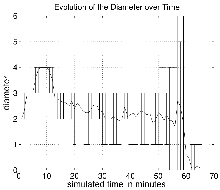
Diameter of the overlay: BitTorrent generates an overlay with a short diameter. As we can observe in Fig. 7, the average diameter of the overlay is between and most of the time11 1 In this paper, we compute the diameter of the overlay as the longest shortest path between peers of the overlay selected at random. This method allows us to obtain very good approximation of the diameter and speeds up the run time of the simulator.. However, at the end time of the torrent, the overlay may get partitioned. If we look closely at the right part of Fig. 7, we notice that the minimum value of the diameter goes to zero, a value we use to indicate partitions. Actually, after a massive departure of peers, we may obtain many small partitions each of tens of peers. The partitions are due to the minimum number of neighbors a peer should reach before recontacting the tracker for new peers. Indeed, to minimize the interaction between peers and the tracker, a peer asks the tracker for more peers only if its number of neighbors falls below . Therefore, as long as the peer set size is larger than , to recover from a decrease in its peer set size, a peer has to wait for new incoming connections from newly arriving peers, which does not happen toward the end of the torrent. That is why the torrent does not merge again. To prevent such a behavior, one needs to assign a high value to . The value of is then a trade-off between having a connected overlay at the end of the torrent, and a high load at the tracker.
In our analysis in Section IV-C, we show that a short diameter is a necessary, but not sufficient, condition for an efficient distribution of the file. We draw in Fig. 8 the shape of the overlay generated by BitTorrent.

We see that BitTorrent does not generate a random overlay, and that the overlay has a specific geometry. Indeed, Fig. 8 shows a clustering among peers that arrive first. For example, peer is connected only to the first hundred peers. The reason is that when arrives, it connects to all the peers already existing in the torrent. Then, waits for new arrivals in order to complete the 56 peers it still needs to saturate its peer set. According to Eq. (2), these missing connections can be fulfilled after the arrival of 75 peers on average, . Similarly, when peer arrives, it establishes up to 40 outgoing connections. However, needs to wait the arrival of a large number of peers in order to complete its 40 incoming connections. This explains why, as compared to , the neighbors of are selected from a larger set of peers (i.e., between and ). Even though we have this clustering phenomena, the overlay does not include bottlenecks. Actually, the number of connections between the first peers and the rest of the network is equal to . Therefore, the BitTorrent has the potential to allow a fast expansion of the pieces.
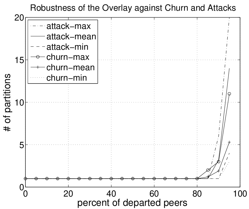
Robustness to attacks and churn: We investigate the robustness of the overlay to a massive departure of peers, which can be due to an attack or a high churn rate. We now consider how we simulate the attack scenario. First, we consider the overlay topology shown in Fig. 8, which represents a snapshot of the topology at time . Then, we force the most connected peers to leave. For example, assume that we want to evaluate the robustness of the overlay to attacks after the departure of of the peers. In this case, we identify the most connected peers in the overlay and we disconnect them from the overlay. Forcing a peer to leave means that we remove all connections between this peer and the rest of the torrent. Once these peers are disconnected, we check whether the overlay becomes partitioned, i.e., includes more than one partition. By varying the percentage of peers that we force to leave, we are able to explore the robustness limits of the BitTorrent overlay.
To simulate a churn rate, we proceed similarly as for the case of an attack. The only difference is that, the peers that we force to leave are selected randomly instead of the most connected ones.
Fig. 9 shows that BitTorrent’s overlay is robust to attacks and churn. Indeed, the overlay stays connected, i.e., there is a single partition, when up to of the peers leave due to an attack or to churn rate. When more than of the peers leave the torrent, partitions appear. However, there is one major partition that includes most of the peers and a few others with one peer each.
For example, when of the peers leave the torrent due to an attack, the result of run produced partitions. More precisely, we had partition that included peers, partitions that included each peers, other partitions with peers each, and partitions with single peer each. Similarly, when of the peers leave the torrent due to a high churn rate, the overlay was split into partitions, partition with peers, partition with peers, and partitions with peer each.
In summary, we have seen that the average peer set size is significantly lower than the maximum peer set size, and the peer set size of a peer depends on its arriving time in the torrent. In addition, BitTorrent generates an overlay with a short diameter, but this overlay is not a random graph. However, the overlay is robust to attacks and churn.
V-B Validation with Experiments
To validate our simulation results, we have run real experiments using the mainline client 4.0.2 and its tracker implementation that we described in details in Section III-B. In Fig. 10(a) and Fig. 10(b) we draw the connectivity matrix of the overlay as obtained from experiments and simulations respectively. The connectivity matrix is computed after the arrival of peers to the network. As we can see from these two figures, the real experiments and the simulations show similar properties of the overlay. As a result, our simulator produces accurate results, and as compared to real experiments, it offers much more flexibility and allows us to consider larger torrents. Therefore, in the following, we will give results only for simulations.


In the next sections, we will investigate how these results are influenced by (1) the size of the torrent, (2) the maximum peer set size, (3) the maximum number of outgoing connections, and (4) the percentage of NATed peers. We will also discuss in Section VI how peer exchange impacts those results.
V-C Varying the Number of Peers
The torrent for the initial scenario is of moderate size. Indeed, it consists of peers and of a maximum of simultaneous peers. To validate how the results of Section V-A are impacted by larger torrents, we have considered two other torrent sizes: and peers. For the largest torrent, the maximum number of simultaneous peers is .

Average peer set size: The average peer set size does not depends on the torrent size. Indeed, Fig. 11 shows that the average peer set size is roughly the same for the three torrent sizes. For example, after 10 minutes, when the number of simultaneous peers is for the smallest torrent and for the largest torrent, the average peer set size is the same for the three torrents. The evolution of the peer set size for the three torrents is similar to the once presented in Fig. 6. The peer set size decreases from for the peers that join the torrent early to around for the peers that arrive toward the end.
Convergence speed: According to section IV-B, the convergence speed of the peer set decreases when the torrent size increases as shown in Fig. 3.

Diameter of the overlay: The diameter of the overlay increases slowly with the torrent size. As we can observe in Fig. 12, after 10 minutes, the diameter of the overlay is for the smallest torrent and for the largest torrent. The connectivity matrix presents the same characteristics as in Fig. 8 for the three torrents.

Robustness to attacks and churn: Fig. 13 shows that the robustness of the overlay is independent of the torrent size. In particular, the three overlays stay connected for up to of peer departures. Then, the overlay is partitioned with a single large partition and several partitions with a few peers. To show the similarity at the robustness level for the different torrent sizes, we now analyze the number of partitions that we obtain with the attack scenario after the departure of of the most connected peers. Our results show that the torrent of peers becomes partitioned into partitions with one partition of peers and three others of one single peer each. Similarly, the torrent of peers becomes partitioned into partitions with one partition of peers and four others of one single peer each. Finally, the torrent of peers becomes partitioned into partitions with one partition of peers, another partition of two peers, and seven other partitions of one peer each. We found the same tendency for the churn scenario.
In summary, we have investigated the impact of the torrent size on the properties of the overlay formed by BitTorrent. We have found that the results obtained for the initial scenario still hold for larger torrents. Therefore, and in order to reduce significantly the run time of these simulations, in the following, we will focus on a torrent with peers.
V-D Impact of the Maximum Peer Set Size
The maximum peer set size is usually set to . However, some clients choose higher values of this parameter, e.g., mainline 5.x [5] has a maximum peer set size set to . In this section, we evaluate the impact of this parameter on the properties of the overlay.
We run simulations with a maximum peer set size varying from to . For each value of , we set the maximum number of outgoing connections to , the number of peers returned by the tracker to , and the minimum number of neighbors to . Then, we evaluate the overlay after simulated minutes, because it is the time at which the number of simultaneous peers in the torrent reaches its upper bound of peers.
Note that there is no specific rule to set the value of the number of peers returned by the tracker when we change the maximum peer set size and maximum number of outgoing connections . Intuitively, should be larger than . The reason is that each peer seeks to initiate connections, which is only possible if the tracker provides with the addresses of at least other peers in the torrent. Yet, the value of should not be much larger than in order not to increase the load on the tracker. We tried several values of between and , but we obtained similar results. Therefore, we decided to set to .

Average peer set size: The average peer set size increases linearly with the maximum peer set size . Indeed, Fig. 14 shows that the average peer set size is roughly equal to . For instance, for a maximum peer set size of , the average peer set size is .
We found this linear trend in all our simulations, but the slope depends on the instant at which we perform the measurements.
Convergence speed: We extend the analysis in Section IV-B by considering a variable maximum peer set size and a maximum number of outgoing connections . We rewrite Eq. (2) as follows:
| (4) |
where is the number of missing connections, i.e., the number of incoming connections the peer is still waiting for, assuming that the peer has succeeded to initiate outgoing connections. is the probability that a peer receives a new incoming connection from a new peer given the number of peers in the torrent. Recall that represents the torrent size at the moment of the arrival of peer , and is the average number of peers that should arrive after peer in order for this peer to complete its missing connections. We assume that no peer leaves the system. When Eq. (V-D) is equivalent to , which is Eq. (2). Therefore, when , the convergence speed is independent of the value of .

Diameter of the overlay: The diameter of the overlay decreases slowly with the maximum peer set size as shown in Fig. 15. The diameter is when is , when is , when is , and when is . However, in contrast to the average peer set size, there is no clear trend that can be used to predict the diameter as a function of the maximum peer set size.

Robustness to attacks and churn: The robustness of the overlay increases with the maximum peer set size as shown in Fig 16. For example, when we set to , , and , the overlay is not partitioned for up to respectively , , and of peers that leave. There is no discernible distinction between leaves due to churn or attacks.
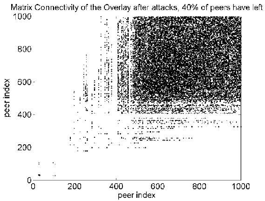
However, if we carefully look at Fig. 16, we can see that the attack scenario produces partitions when the percentage of departed peers is at . To understand this behavior, we plot in Fig. 17 the connectivity matrix of the overlay after attacking of the peers. Fig. 17 shows that there are around peers that are disconnected from the rest of the torrent.
From our previous results, we know that the peers that arrive at the beginning of the torrent are the most connected ones and highly connected among each other (see Fig. 8). In addition, these first peers are the most concerned ones by the attack. Recall that the attack scenario forces the most connected peers to leave the torrent. Thus, with a of departed peers, only very few of those first peers will remain present in the torrent after the attack. These few peers will have a very few neighbors and will become disconnected from other peers. However, if we consider a percentage of departed peers of instead of , more peers will leave the torrent and those peers will disappear. This means that the torrent will be connected again. In contrast, if we consider a percentage of departed peers of instead of , there will be more peers present in the torrent after the attack, which helps the torrent to remain connected.
In summary, the maximum peer set size does not have a major impact on the properties of the overlay, as long as the maximum peer set size is large enough to have a small diameter. In our simulations, we do not see a major difference in the overlay properties between a maximum peer set size of and . However, as the maximum peer set size increases linearly the average peer set size, it also increases the speed of replication of the pieces (according to Section IV-A). Therefore, the main reason to increase the maximum peer set size is to improve the speed of replication. But, there is a tradeoff, as a larger maximum peer set size increases the load on each client due to the larger number of TCP connections to maintain and due to the signaling overhead per connection.
V-E Impact of the Maximum Number of Outgoing Connections
The maximum number of outgoing connections is critical to the properties of the overlay. Indeed, when is close to the maximum peer set size , the peer set size will converge fast to , but new peers will find few peers with available incoming connections, hence a larger diameter.
In this section, we evaluate the impact of on the overlay properties. For the simulations, we set to , the minimum number of neighbors to , and we vary from to with a step of . For each value of and , the number of peers returned by the tracker is equal to .

Average peer set size: Fig. 18 shows the evolution of the average peer set size as a function of the maximum number of outgoing connections. We see that the average peer set size increases fast with when is smaller than , and it increases slowly with when is larger than . We notice that, a small leads to a small average peer set size. For example, when is equal to , the average peer set size is around .

Convergence speed: In Fig. 19 we plot the peer set size of each peer at time minutes as a function of the peer id for three values of the maximum number of outgoing connections. These outdegree distributions of peers reflect the convergence speed of peers towards their maximum peer set size. As we can see from Fig. 19, the peer set size of the different peers improves with when is smaller than , and it increases slowly with when is larger than . For example, after the arrival of the first peers , peer has a peer set size of when is at and a peer set size of when is at . However, when we increase from to , the peer set size of increases from to only. This result means that, when we increase beyond , the convergence speed of a peer towards its maximum peer set increases slowly. We explain this conclusion as follows. According to Eq. (V-D), when increases, decreases, where is the number of peers that should arrive after a peer , so that reaches its maximum peer set size. Indeed, when increases, the probability that a peer receives incoming connections from new peers increases too. However, to derive Eq. (V-D), we assumed that a peer succeeds to establish all its allowed outgoing connections and that the number of connections it misses is . This is the most optimistic case, and it is not true when is larger than . Indeed, in that case, peers that arrive at the beginning of the torrent are able to establish a lot of connections among themselves and reach fast their maximum peer set size. However, those peers leave few rooms for incoming connections, as is close to the maximum peer set size . Therefore, peers that join later the torrent will not be able to establish outgoing connections, which results in a larger number than of missing connections. As a consequence, the increase in the probability that a peer is selected by new arriving peers is compensated by the increase in the number of missing connections.


Diameter of the overlay: Taking a maximum number of outgoing connections larger than increases the diameter of the overlay. As we can see in Fig. 21, for equal to (respectively ), the diameter of the overlay is equal to (respectively ). When is equal to , i.e., 80, the overlay is partitioned. If we focus on the connectivity matrix of the overlay, we observe how the overlay gets partitioned into two partitions. Indeed, Fig. 20(a) shows that when is equal to 70, the connectivity matrix becomes narrow around peer index 80. This results in the first peers in the torrent being highly connected among themselves with connections, and poorly connected with the rest of the torrent with connections. When is equal to 80, the first 80 peers become disconnected from the rest of the torrent. This might be a major issue if the source of the torrent is among those 80 peers, which is the regular case.

Robustness to attacks and churn: Fig. 22 draws the robustness of the overlay with a maximum number of outgoing connections set to , , and . We observe that large values of make the overlay slightly more robust to attacks and churn. For example, in case of an attack, when setting to , the partitions appear after the departure of of the peers. In contrast, when setting to or , the partitions appear after the departure of of the peers.
In Fig. 22, we can also show that, when we set of , the number of partitions decreases at the end of the curve. The reason is that, when we force or more of the most connected peers to leave the network, a of will produce a lot of partitions with a very few peers each. Thus, increasing the number of departing peers removes those “one single peer partitions”.
Note that, when is set to (respectively to ), the attack scenario produces partitions when the percentage of departed peers is at (respectively ). The reason is that, among the most connected peers, the remaining peers are very few to stay connected with the rest of the torrent.
In summary, setting the maximum number of outgoing connections to is a good tradeoff between the average peer set size and the diameter of the overlay.
V-F Impact of the Number of NATed Peers
In this section, we discuss the impact of the percentage of NATed peers on the overlay properties. When a peer is behind a NAT, it cannot receive incoming connections from other peers in the torrent. However, it can initiate outgoing connections to non NATed ones. For the simulations, we set the maximum peer set size to , the maximum number of outgoing connections to , the minimum number of neighbors to , and the number of returned peers by the tracker to . Then, we vary the percentage of NATed peers from to with steps of .

Average peer set size: BitTorrent mitigates very efficiently the impact of the NATed peers on the overlay. For example, we see in Fig. 23 that as we increase the percentage of NATed peers from to , the average peer set size is reduced from to . Indeed, the average peer set size decreases slowly with the percentage of NATed peers. However, the slope of the curve becomes much sharper when the percentage of NATed peers exceeds .
Convergence speed: The convergence speed that we derive in Eq. (2) holds for non NATed peers. When a peer is NATed, it will establish at most outgoing connections, which is the higher bound for its maximum peer set size.

Diameter of the overlay: NATed peers do not make the diameter significantly larger. For example, as shown in Fig. 24, when (respectively of the peers are NATed, the average value of the diameter is at (respectively ). However, in extreme cases where of the peers are NATed, the diameter can reach .
Note that, NATed peers may cause partitions. For example, assume that peer is NATed. It may happen that, out of the peers returned by the tracker to , no one has room for more connections. As a result, will not be able to establish any outgoing connections. In addition, and because it is NATed, cannot receive connections from other peers. As a result, peer will be isolated alone (disconnected from the rest of the torrent) until it contacts the tracker again and discovers more peers. This behavior becomes more common as the percentage of NATed peers increases.

Robustness to attacks and churn: The robustness of the overlay to high churn rates does not depend on the presence of NATed peers. Indeed, Fig. 25 shows that the overlay stays connected when up to of peers leave the torrent. However, the overlay is not robust to attacks when there is a large number of NATed peers. Indeed, Fig. 25 shows that when there are of NATed peers, the overlay starts to be partitioned when of the peers leave due to an attack. We see that the number of partitions decreases for a large percentage of departing peers, because as there are many small partitions, increasing the number of departing peers removes those partitions.
In summary, NATed peers decrease significantly the robustness of the overlay to attacks.
VI Impact of Peer Exchange on the Overlay
We have seen that BitTorrent generates overlays with a short diameter that are robust to churn and attacks. However, the time for a peer to reach its maximum peer set size depends on the torrent size and peer arrival rate. One way to reach faster the maximum peer set size is to increase the number of requests to the tracker in order to discover more peers and establish more connections. However, such requests increase the load on the tracker, whereas the tracker is known to have scarce resources [18, 19].
In Mai , Azureus 2.3.0.0 [20] introduced a new feature, namely peer exchange (PEX), where neighbors periodically exchange their list of neighbors. For example, assume that peers and are neighbors. Then, every minute, sends its list of neighbors to and vice versa. As a result, each peer knows its neighbors and the neighbors of its neighbors. The intuition behind PEX is that peers will be able to discover fast a lot of peers and consequently achieve a larger peer set size.
Note that the results that we have given in previous sections are for the case of BitTorrent without PEX, e.g., the official BitTorrent client [5]. In this section, we extend our work and analyze how PEX impacts the overlay topology of BitTorrent. PEX is becoming very popular and, in addition to Azureus, it is now implemented in several other P2P clients including KTorrent, libtorrent, Torrent, or BitComet, but with incompatible implementations. To the best of our knowledge, the impact of PEX has never been discussed previously.
VI-A Simulating PEX
To evaluate the impact of PEX on the overlay topology, we added this feature to our simulator exactly as it is implemented in Azureus. Concerning the communications between peers and the tracker, all what we described in Section III-B is still valid. That is, the tracker keeps two lists, and peers. And, when a peer joins the torrent, it gets from the tracker up to peers randomly selected from . Then, stores those IP addresses in its list and initiates sequentially up to connections to those peers. Moreover, will be added at the tracker to either or .
We now explain the modifications that we made in our simulator. Assume that, at time , a connection has been established between two peers and . Just after, sends its list of neighbors to and vice versa. Then, every simulated minute, and repeat this exchange process.
Assume now that, after performing PEX with its neighbor , discovers peer . Then, checks whether (1) it already has a connection with or (2) it already knows from the tracker. If none of these two conditions holds true, then adds to the list of peers it discovered through PEX. Note that, may receive the IP address of from many neighbors. In this case, will appear only once in .
Note that, when establishing connections, peers discovered from the tracker are given more priority. For example, assume that peer decides to initiate a new connection, which can be due to the departure of one of its neighbors or after discovering new peers. In this case, contacts first the peers it has discovered from the tracker. If none of those peers accepts the connection request, contacts the peers that it discovered through PEX.
VI-B Analysis of PEX
We implement PEX in our simulator and run simulations with the following parameters. We set the maximum peer set size to , the maximum number of outgoing connections to , the minimum number of neighbors to , and the number of peers returned by the tracker to . However, due to the gossiping messages between peers, the PEX feature makes our simulator very slow. In order to save time, we run simulations for a torrent of peers that arrive to the torrent within the first simulated minutes according to Eq. 1. The departure of peers is scheduled during the next simulated minutes, and it follows a random uniform distribution. For example, if peer arrives at time , it will leave the network at a random time uniformly selected between and . Still, this torrent allows us to understand how the overlay is constructed with PEX and how it evolves as peers join and leave.

Average peer set size: PEX meets its intended goal and permits peers to be at their maximum peer set size most of the time as shown in Fig. 26. Moreover, PEX prevents the average peer set size from decreasing in case of a massive departure of peers. Indeed, when a peer loses a connection due to the departure of a neighbor, it can replace it by a new connection to one of its neighbors’ neighbors. As a result, the average peer set size stays at its maximum value of as long as there are peers in the torrent.
Convergence speed: Each peer reaches its maximum peer set size within a few gossiping period (that we set to one minute in our simulations).


Diameter of the overlay: The increase in the average peer set size comes at the expense of a larger diameter. As we see in Fig. 27, the maximum value of the diameter reaches when the number of peers in the torrent is .
To explain why PEX produces such a long diameter, we plot in Fig. 28 the evolution of a torrent with 9 peers () that arrive sequentially, one every 1 unit of time. In this example, we set the maximum peer set size to 4, the maximum number of outgoing connections to 2, and the number of peers returned by the tracker to 2. At time , there is only peer . At time , joins the torrent and connects to . At time , arrives and connects to and . Then, arrives and connects to two existing peers selected at random, say and . At the end of time , PEX has not yet been used. At time , arrives and connects to and , which in turn tell and about this new neighbor. At this time, and each has a room for one more outgoing connection and both connect to . Thus, at time , only peers and can accept new incoming connections, i.e., , , and have already reached the maximum number of connections. At time , peer joins the torrent and gets from the tracker the addresses of and . However, can only initiate a connection to , as has already reached its maximum peer set size. Peer arrives at time , gets the addresses of and and initiates one connection to . Then, joins the torrent at time , obtains the addresses of and and initiates only one connection to . At time , peer arrives and gets the addresses of and . Given that these two peers have not reached their maximum peer set size, succeeds to connect to both of them. Afterward, tells its neighbor about , thus a new connection is initiated from to . Then, tells about and a new connection is initiated from to .
As we can see, PEX tries to maximize the number of outgoing connections at each peer. Peers keep on gossiping and whenever they discover new peers, they establish new connections if they still have room for. However, the disadvantage is that peers that arrive at the beginning establish a lot of connections among each other and leave only a few free connections for the peers that arrive afterward. In the example that we consider here, are highly interconnected and they leave only two connections for next peers. Similarly, when peers arrive, they connect to the overlay at peers and and then interconnect strongly with each other.

As a result, PEX leads to a clustering phenomena, where each cluster contains approximately a number of peers close to the maximum peer set size. Each cluster exhibits a high intra-cluster connectivity and a poor inter-cluster connectivity with the cluster that arrives just before and to the one that arrives just after. To confirm our analysis, we draw in Fig. 29 a snapshot of the connectivity matrix of the overlay distribution after minutes when the first peers have arrived in the torrent. The clustering phenomena appears clearly in the figure, which explains the large diameter of the overlay. As we explained in Section IV-C, such a chain-like overlay constraints the distribution time in the system to be a linear function of the number of clusters. As compared to the overlay generate by the tracker only, this chain-like overlay becomes less efficient when the number of clusters becomes larger than the number of pieces. Typical files distributed using BitTorrent includes an average of pieces. In this case, this chain-like overlay will become inefficient when the number of clusters is larger than , i.e., the number of peers is larger than peers. Current torrents are much smaller and they rarely exceed 100.000 peers and therefore, no one has noticed yet the negative impact of the PEX on the download time of files.
Let us now go back to Fig. 27. If we carefully look at this figure, at time minutes, the average value of the diameter drops from to . Actually, at minutes, peers start leaving the torrent. At the same time, the last peers to join the torrent also arrive at minutes. Those departed peers will allow the arriving ones to connect at different levels of the chain and not only at the tail, which consequently reduces the diameter of the overlay.
To better explain this behavior, consider the overlay shown in Fig. 29. In this chain-like overlay, all peers are at their maximum peer set size except those that are at the tail. Assume now that peers leave the torrent. Assume that, at the same time, join the torrent. In this case, the departed peers will leave rooms for incoming connections inside the first cluster, i.e., at the head of the chain. Thus, the arriving peers will be able to establish connections to the tail as well as the head of the chain. As a result, the head and tail of the chain become connected and the diameter of the overlay drops by half. Still, the diameter remains very high when compared to an overlay generated only by the tracker.


Robustness to attacks and churn: Surprisingly, the overlay produced with PEX is robust to churn rate and to the attack that targets the most connect peers. As shown in Fig. 30(a) and Fig. 30(b), the overlay stays connected with up to of the peers leaving the torrent.
As we can see in Fig. 30(a), up to of departed peers, the attack scenario produces a maximum number of partitions of . Actually, out of the ten runs that we performed, we obtained partitions with only run. In particular, we obtained one major partition and a second one with only peer. For example, for of departed rate, we obtained partition that includes peers and a second partition with only peer. Same conclusions apply on the churn scenario.
Even though PEX shows good robustness to the attack that we have been using so far, this chain-like overlay can be easily partitioned by using more sophisticated attacks that target a peer, its neighbors, and its neighbors of neighbors.
In summary, even if PEX significantly decreases the time for a peer to reach its maximum peer set size, it creates a chain-like overlay that is not robust against partitions and whose diameter is large. This large diameter will lead to a long download time of files when the number of simultaneous peers is large. We plan to evaluate how much this overlay impacts the efficiency of the transfer when compared to an overlay created only by the tracker.
VII Discussion
VII-A Summary of our Contributions
We have conducted a large set of simulations to investigate the properties of the overlay formed by BitTorrent. Below is a list of our main contributions.
- •
First, we have analyzed the relation between the overlay properties and the performance of BitTorrent. In particular, we have shown that a large peer set size increases the efficiency of BitTorrent, and that a small diameter is a necessary, but not sufficient, condition for this efficiency.
- •
Second, we have shown for the first time that the overlay generated by BitTorrent is not a random graph, as it is commonly believed. The connectivity of a peer with neighbors in the torrent is highly biased by its arriving order in the torrent. Whereas it is beyond the scope of this study to evaluate the robustness of the overlay structure to elaborated attacks, i.e., attacks that do not only focus on the most connected peers, it is an interesting area for future research. In particular, it is critical to understand such issues when a public service is to be built on top of BitTorrent.
- •
Third, we have evaluated the impact of the maximum peer set size and of the maximum number of outgoing connections. Whereas there are several magic numbers in BitTorrent, we have identified that the maximum peer set size is a tradeoff between efficiency and peers overhead, and we have explained why the maximum number of outgoing connections must be set to half of the maximum peer set size.
- •
Finally, we have identified two potentially significant problems in the overlay, which deserve further investigations. We have shown that a large number of NATed peers decrease significantly the robustness of the overlay to attacks, and we have shown that peer exchange creates a chain-like overlay that might adversely impact the efficiency of BitTorrent.
In conclusion, we expect this study to shed light on the impact of the overlay structure on BitTorrent efficiency, and to foster further researches in that direction.
VII-B Future Work
Our future work will progress along two avenues.
- •
Mitigate the impact of NATed peers on the robustness of the overlay. Actually, with its current implementation, BitTorrent produces an overlay where non-NATed peers have a higher connectivity than NATed ones. As a result, one can create partitions by attacking the non-NATed peers, which are the most connected ones. One possible solution to this problem is to allow NATed peers to initiate more connections than non-NATed ones. For example, one can imagine that the tracker reports the number of NATed peers to new peers so that they can weight their maximum number of outgoing connections. Our goal is to still have a highly connected graph, but without peers with significantly more connections. The intuition behind this solution is that the robustness of the overlay would improve. This solution, and in particular how to weight the maximum number of outgoing connections, will be subject to further investigation.
- •
Extend peer exchange in order to still converge fast to the maximum peer set size while maintaining a low diameter overlay. Indeed, with the current implementation of peer exchange, peers converge fast to their maximum peer set size, but only peers that are at the tail of the overlay chain have rooms for incoming connections. As a result, new arriving peers can only connect to the tail of the overlay chain. We are investigating possible solutions to this problem whose main goal is to add randomness in the overlay generated with peer exchange.
One solution is to allow peers coming from the tracker to preempt connections of peers discovered with peer exchange. For example, assume that peer has reached its maximum peer set size and amongst its neighbors, there is that it discovered with peer exchange. Assume now that joins the torrent and receives the IP address of from the tracker. If initiates a connection to , will accept this connection and drop its connection to .
Another solution is to add randomness during the construction of the overlay. For instance, instead of collecting a list of neighbors of its neighbors, which creates locality in the graph construction, a peer can ask neighbors to randomly selected peers. The rational is to discover and create connections to peers that are far from in the overlay. The choice of the random function to discover those peers is critical and currently under investigation.
Acknowledgments
We would like to thank Olivier Chalouhi, Alon Rohter, and Paul Gardner from Azureus Inc. for their information on peer exchange.
References
- [1] Y. H. Chu, S. G. Rao, and H. Zhang, “A case for end system multicast,” in Proc. of ACM SIGMETRICS, Santa Clara, CA, USA, June 2000, pp. 1–12.
- [2] B. Hill, “P2P: 70-80 percent of all euronet traffic,” The Digital Music Weblog, May 2004, http://digitalmusic.weblogsinc.com/.
- [3] B. Cohen, “Incentives to build robustness in Bittorrent,” in Proc. of the Workshop on Economics of Peer-to-Peer Systems, Berkeley, CA, USA, June 2003, http://bitconjurer.org/BitTorrent.
- [4] “BitTorrent beats Kazaa, accounts for 53% of P2P traffic,” AlwaysOn Site, July 2004, http://www.alwayson-network.com/index.php.
- [5] “Bittorrent, inc,” http://www.bittorrent.com.
- [6] A. Legout, G. Urvoy-Keller, and P. Michiardi, “Rarest first and choke algorithms are enough,” in Proc. of IMC, Rio de Janeiro, Brazil, October 2006.
- [7] A. Legout, N. Liogkas, E. Kohler, and L. Zhang, “Clustering and sharing incentives in bittorrent systems,” in Proc. of SIGMETRICS, San Diego, CA, USA, June 2007.
- [8] T. Locher, P. Moor, S. Schmid, and R.Wattenhofer, “Free riding in bittorrent is cheap,” in Proc. of HotNets-V, Irvine, CA, USA, November 2006.
- [9] Y. Tian, D. Wu, and K.-W. Ng, “Modeling, analysis and improvement for bittorrent-like file sharing networks,” in Proc. of INFOCOM, Barcelona, Spain, April 2006.
- [10] M. Izal, G. Urvoy-Keller, E. W. Biersack, P. A. Felber, A. A. Hamra, and L. Garcés-Erice, “Dissecting bittorrent: Five months in a torrent’s lifetime,” in Proc. of PAM, Juan-les-Pins, France, April 2004.
- [11] L. Guo, S. Chen, Z. Xiao, E. Tan, X. Ding, and X. Zhang, “Measurement, analysis, and modeling of bittorrent-like systems,” in Proc. of IMC, New Orleans, LA, USA, October 2005.
- [12] D. Qiu and R. Srikant, “Modeling and performance analysis of bittorrent-like peer-to-peer networks,” in Proc. of SIGCOMM, Portland, Oregon, USA, August 2004.
- [13] G. Urvoy-Keller and P. Michiardi, “Impact of inner parameters and overlay structure on the performance of bittorrent,” in Proc. of Global Internet Symposium, Barcelona, Spain, April 2006.
- [14] N. Liogkas, R. Nelson, E. Kohler, and L. Zhang, “Exploiting bittorrent for fun (but not profit),” in Proc. of IPTPS, Santa Barbara, CA, USA, February 2006.
- [15] Http://planete.inria.fr/software/BitSim/.
- [16] D. Stutzbach and R. Rejaie, “Characterizing the two-tier gnutella topology,” in Proc. of SIGMETRICS ’05, Banff, Alberta, Canada, June 2005.
- [17] X. Yang and G. de Veciana, “Service capacity of peer-to-peer networks,” in Proc. of INFOCOM, Hong-Kong, China, March 2004.
- [18] G. Neglia, G. Reina, H. Zhang, D. Towsley, A. Venkataramani, and J. Danaher, “Availability in bittorrent systems,” in Proc. of INFOCOM, Anchorage, Alaska, USA, May 2007.
- [19] J. Pouwelse, P. Garbacki, D. Epema, and H. Sips, “The bittorrent p2p file-sharing system: Measurements and analysis,” in Proc. of IPTPS, Ithaca, NY, USA, February 2005.
- [20] “Azureus,” http://sourceforge.net/projects/azureus/.