Can Strong Gravitational Lensing Constrain Dark Energy?
Seokcheon Lee 1 and Kin-Wang Ng 1,2
1Institute of Physics,
Academia Sinica,
Taipei, Taiwan 11529, R.O.C.
2Institute of Astronomy and Astrophysics,
Academia Sinica, Taipei, Taiwan 11529, R.O.C.
Abstract
We discuss the ratio of the angular diameter distances from the source to the lens, , and to the observer at present, , for various dark energy models. It is well known that the difference of s between the models is apparent and this quantity is used for the analysis of Type Ia supernovae. However we investigate the difference between the ratio of the angular diameter distances for a cosmological constant, and that for other dark energy models, in this paper. It has been known that there is lens model degeneracy in using strong gravitational lensing. Thus, we investigate the model independent observable quantity, Einstein radius (), which is proportional to both and velocity dispersion squared, . values depend on the parameters of each dark energy model individually. However, for the various dark energy models, is well within the error of for most of the parameter spaces of the dark energy models. Thus, a single strong gravitational lensing by use of the Einstein radius may not be a proper method to investigate the property of dark energy. However, better understanding to the mass profile of clusters in the future or other methods related to arc statistics rather than the distances may be used for constraints on dark energy.
1 Introduction
Recent observations of high redshift Type Ia supernovae (SNe Ia) suggested that the expansion of the Universe is currently accelerating [1]. The cosmic microwave background (CMB) anisotropy data, indicating a spatially flat universe [2] containing a low value for the cold dark matter (CDM) density parameter [3], has confirmed that the Universe is dominantly made up of a component with negative pressure (dark energy) to make up the critical density today.
The cosmological constant and/or a quintessence field are the most commonly accepted candidates for dark energy. Although the cosmological constant is simple and favored by current cosmological observations, there is to orders of magnitude discrepancy between theory and the measured value [4]. The quintessence, which might alleviate this problem is a dynamical scalar field leading to a time dependent equation of state parameter [5]. Various scalar field potentials for the quintessence have been investigated [6].
It is important to use various ways of checking for the existence of dark energy in addition to SNe Ia and CMB anisotropy constraints on dark energy. A number of other tests have been considered including “geometric” tests using standard cosmological methods (the galaxy cluster gas mass fraction [7], the location of CMB peaks [8, 9], the redshift-angular size [10], the strong gravitational lensing [11] - [14], fluctuations of the luminosity distance [15], etc.).
The statistics of gravitational lensing of quasars (QSOs) by intervening galaxies can constrain on the cosmological constant [12]. Lensed images of distant galaxies in cluster, arcs or rings, may provide a bound on the equation of state parameter of dark energy [13]. While SNeIa is used to determine the luminosity distance itself, a gravitational lensing system can be used measure the ratio of angular diameter distances. Thus, the gravitational lensing system is regarded as an independent tool that complements SNe Ia as a probe of dark energy [14].
However, the lensing observations primarily depend on the parameters of lens models with minor dependence on cosmological parameters [16]. There is the lens model degeneracy in both the projected mass density profile and the circular velocity profile. It is shown that we need to measure the Einstein radius and the velocity dispersion within % accuracy in order to put a constraint on .
In the gravitational lensing, one of the observable quantities without having any model dependence is the Einstein radius (), which is proportional to the velocity dispersion squared () and the ratio of the angular distances , where is the distance from the lens to the source and is that from the source to the observer. With different values of cosmological parameters, we can have different values of , i.e. different values of . Thus, it might be used for probing the property of dark energy, . However, there is an ambiguity in measuring . If the error of measurement is not within the differences of between different cosmological models, then we cannot distinguish the differences between models by measuring .
This paper is organized as follows. In the next section we review the gravitational lensing system with the basic equations used in lensing observations. We also briefly mention the most popular lens models. We review the various aspects of errors in modeling lens in Sec. . In Sec. , we check both the differences of and the differences of between the cosmological constant and other dark energy models. Our conclusion is in the last section.
2 Gravitational Lensing and Isothermal Galaxy Models
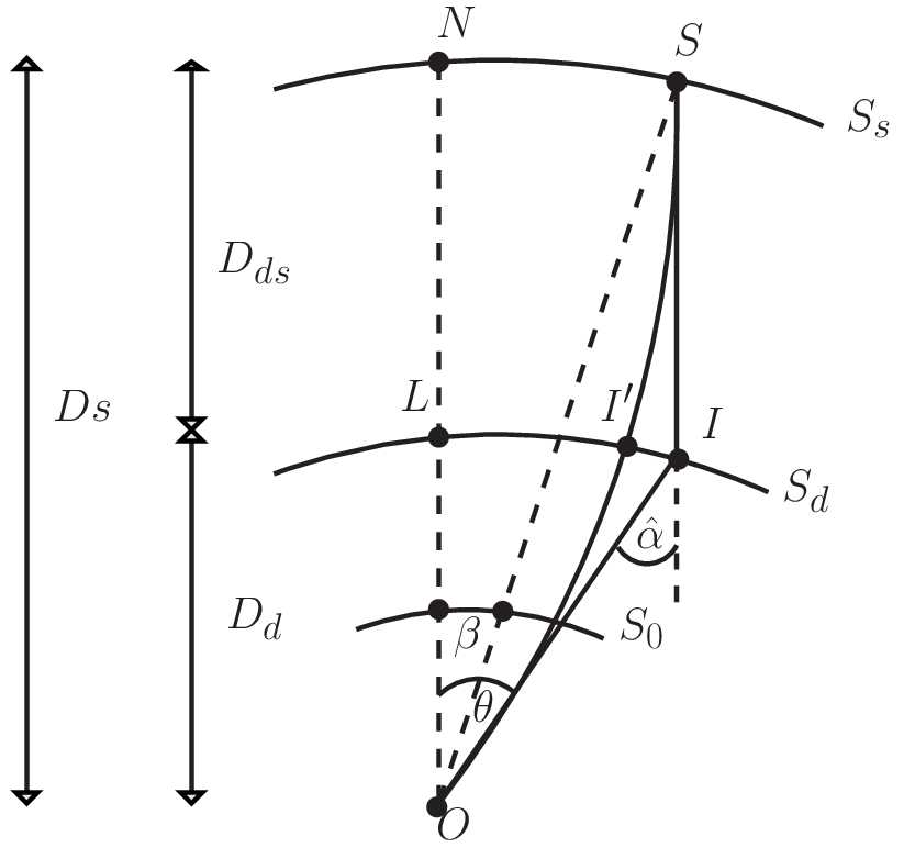
Figure 1 shows a simple lensing system [17]. Consider the source sphere , i.e. a sphere with radius , centered at the observer and the deflector sphere with radius , i.e. the distance to the center of the lens . In addition, consider the observer sphere where the source would have angular position (bold faced characters represent -dimensional vectors in this manuscript) if the light rays from the source were not influenced by the gravitational field of the deflector. However, since light rays are bent by the lens, the straight line is no longer a physical ray path. Rather, there are light rays which connect the source and the observer but they are curved near . One such ray is drawn, together with its approximation , consisting of the two asymptotes of the real ray. The separation of the light ray from the optical axis, , is defined as the impact vector in the lens plane. The angle between the two asymptotes and is the deflection angle caused by the matter distribution ,
| (2.1) |
where the integral is over the lens plane and is the surface matter density at position resulting from the projection of the volume mass distribution of the deflector onto the lens plane. This is valid when the gravitational field is weak, hence the deflection angle is small. The observer will thus see the source at the position on his sphere .
From the geometry of Fig.1, we can easily derive a relation between the source position described by the unlensed position angle and the position of the images of the source
| (2.2) |
We can reexpress this equation by using the distance from the source to the optical axis as
| (2.3) |
It is useful to rewrite lens equations (2.2) and (2.3) in dimensionless form by introducing a length scale in the lens plane, which is called as the Einstein radius in the lens plane and a corresponding length scale in the source plane. The Einstein radius in the lens plane is given by
| (2.4) |
where is the mass of the lensing object. By use of the definition of the dimensionless vectors and as well as the dimensionless surface mass density (convergence) where the critical surface matter density , the lens equations are rewritten as
| (2.5) |
where is the scaled deflection angle,
| (2.6) |
and is defined as
| (2.7) |
If the lensing object is a point mass, then the cross section for strong lensing events is given by [18]
| (2.8) |
We need to specify the mass distribution to solve the lens equation (2.5). One simple and analytic solution of a differential equation for the radial mass distribution is the singular isothermal sphere (SIS) [18]. Its surface mass density, projected onto the lens plane, is given by
| (2.9) |
where is the velocity dispersion along the line of sight and the length scale . With these we get the lens equation
| (2.10) |
with the convergence
| (2.11) |
Due to its simplicity and the consistency with the matter distribution of galaxies, the SIS is frequently used as the gravitational lens model. In addition to SIS, a nonsingular isothermal sphere (NIS), the singular isothermal ellipsoid (SIE) and Navarro-Frenk-White (NFW) [19] are the most commonly used gravitational lens models. All of them are distinguished by their own surface mass densities as in the equation (2.9).
3 Errors in Modeling Lens
In this section we review systematic errors in the ratio [14]. As we mentioned in the previous section, the various isothermal galaxy models are specified by their surface mass densities (), which are the function of the velocity dispersion () along the line of sight. Isothermal ellipsoid models (SIE, NIE) have an additional necessary measurement, the ratio of the minor axis to the major axis, , which is related to the ellipticity by
| (3.1) |
The lens equation gives an elliptical image of the Einstein ring with the minor and major axes
| (3.2) |
where
| (3.3) |
as given in Eq. (2.4). Thus can be determined by measuring , , and .
Even though gravitational lensing has been used as a useful cosmological tool to probe the high redshift universe, there are several problems. Observational quantities depend on a lens model, which has inherent uncertainties in itself [20]. In most cases, we do not know the property of the lensing object in detail. Also, the light propagates through the local inhomogeneous spacetime which deviates from the smoothed Robertson-Walker metric. Thus, even though the global parameters such as the energy density parameters are fixed, the distance formula is not uniquely determined [21]. In spite of all these ambiguities, if dark energy dominates over the mass density, then the optical depth increases dramatically and its effect is much larger than the uncertainty arising from the problems in the formulation [22]. However in the following section we investigate the model independent observable quantity, Einstein radius.
4 Angular Diameter Distances
In this section, we investigate the ratio of the angular diameter distances from the lens to the sources () and those from the source to the present observer () for various dark energy models. We consider a spatially flat, homogeneous, and isotropic universe with radiation, matter, and dark energy.
The angular diameter distance from the observer at present to the source, , is defined as
| (4.1) | |||||
where is the luminosity distance and is the redshift when radiation and matter densities are equal. In the following numerical calculations, we use . The angular diameter distance depends on the present values of energy density contrast of matter () and dark energy () and the equation of state of dark energy () as in Eqs. (4.1) and (4.2). In a flat universe, we have the constrain when we use the fact that . Especially, dark energy is the cosmological constant () when and we call the model including cold dark matter and cosmological constant as CDM model.
However , itself may not be an interesting quantity in the study of gravitational lensing. Instead, we need to know the combination of angular diameter distances. We want to investigate the least model dependent observable quantity for our study and Einstein radius is one of the proper objects for this purpose. We can represent the angular diameter distance from the lens to the source as
| (4.2) |
where we assume .


If we rewrite the Einstein radius, Eq. (3.3), then the ratio of the angular diameter distances is given by
| (4.3) | |||||
Thus, the error that contributes to this ratio due to the error from the velocity dispersion is
| (4.4) |
We will not consider any detail of the lens model, which can arise additional errors. From various sources of the lens system, we can roughly say that the error of the velocity dispersion is about % (%) [23]. That means we can distinguish the differences between models if the difference of the ratio of the angular diameter distances between models, is at least %. Now we will compare the differences of the ratios of angular diameter distances for different models. There was a work related to this approach [24]. However in the previous work, the equation of state parameter of dark energy was constrained as a constant. We consider more general cases with the stronger constraint on constant s.
4.1 when constant


We assume that the stand cosmological parameters are and and we denote the ratio of the angular diameter distances with these parameters as . Figure 2 shows the difference of between the standard case and the various constant equation of state cases, . In the left panel of Fig. 2, we show the dependence on for different values of , (solid line), (dotted line), and (dash-dotted line). If there is an error in measuring within the range (, ) for ), then is less than %. For example, if the measured cosmological parameters are and , then we cannot distinguish this with the standard case, ( and ) within % by using , i.e. by measuring . also varies for different values of , so does not necessarily have smaller difference to the standard case as can be shown in the left panel of Fig. 2. When , we can have the standard case if . In this case . This is shown in the left panel of Fig. 2 and it shows the consistency of figures. We show dependence on for different values of , (solid line), (dotted line), and (dash-dotted line) in the right panel of Fig. 2. Again if there is an error in measuring within the range (, ) for ), then is less than %. For example, if the measured cosmological parameters are and , then we cannot distinguish this with the standard case within %. We can also see that when and in the right panel of Fig. 2.
We show the dependence of on the position of source () in the left panel of Fig. 3 for different values of (solid line), (dotted line), and (dash-dotted line). We choose the position of lens as and . If we choose for different values of , then we have the same values of of the dotted line of the right panel of Fig. 2. If the source position of lensing system is located () for (), then is less than %. We cannot distinguish the difference of s between the standard case and within % independent of the source position. In the right panel of Fig. 3, we show the dependence of on the position of lens () when we choose and with the same notation as the left panel of the figure for the different values of . When we vary from to for every values of (), s are well below %. To check the consistency between the figures, we can check values when we choose in the right panel of Fig. 2. This gives (, ) when ), which is equal to value when we choose in the left panel of the same figure.


4.2 when
Now we check the difference of the ratio of the angular diameter distances between the standard case and one of the time varying models, [25]. We define where means value when we use . We assume that there is no error in the measured value of in this case. We show dependence on value for different values of , (solid line), (dotted line), and (dash-dotted line), respectively in the left panel of Fig. 4. is within % for () when (). For example, when and , then we cannot distinguish the cosmology with the cosmological constant from the cosmological model with time varying dark energy within % by using . In the right panel of Fig. 4, we show the dependence of for different values of , (solid line), (dotted line), and (dash-dotted line). When varies from to every value is within % for every value of from to . For the consistency check we can choose for three different lines. We can check these values with the three different points of solid line of the left panel of the figure. When we choose , , and for , and in both left and right panels of Fig. 4.


We again check dependence on the position of and for the various sets of and values in figure 5. In the left panel of Fig. 5, we show dependence on . We choose and in this case. For the given sets of and values, we cannot distinguish the cosmological model with the cosmological constant from the cosmological model with time varying dark energy no matter where the source of lens is located from to within % by measuring . We check dependence on for the same sets of and in the right panel of Fig. 5. We choose . Again none of case can be distinguished with cosmological constant case within %.


4.3 when
We check another time varying dark energy model by using the parameter in figure 6. We define where means value when we use [6]. The angular diameter distance of this parametrization is almost degenerate with that of the cosmological constant. Thus, the ratio difference of angular diameter distances between this parametrization and the cosmological constant is extremely small for the different choice of parameters. We choose , , and in this figure. In the left panel of Fig. 6, we show the dependence of on for the different values of , (solid line), (dotted line), and (dash-dotted line). For all of the cases, are within % for different values of from to . In the right panel of Fig. 6, we show dependence on for different values of , (solid line), (dotted line), and (dash-dotted line). Except for case, are degenerate within %. Thus, we cannot tell any difference between the cosmological constant and the dark energy with the parameter by measuring within %.
We again check dependence on the position of and for various sets of and values in Fig. 7. In the left panel of Fig. 7, we show dependence on . We choose and in this case. For given sets of (, ) values, (, ) (solid line), (, ) (dotted line), and (, ) (dash-dotted line), we cannot distinguish the cosmological model with the cosmological constant from the cosmological model with time varying dark energy no matter where the source of lens is located from to within % by measuring . We check dependence on for the same sets of and in the left panel of the figure. We choose . Again none of the cases can be distinguished from the cosmological constant case within %.


5 Conclusions
We have investigated the angular diameter distances from the source to the present observer for the various dark energy models. The angular diameter distance is proportional to the luminosity distance, which is used for the analysis of Type Ia supernovae. The difference of between models is apparent and measuring this quantity as to probe dark energy models might be proper for further investigation. In addition to SNeIa, the gravitational lensing has been known as the possible method to probe the property of dark energy.
Most of the lensing analyses have the Einstein radius as a basic quantity. This is lens model independent observable quantity and might be a good probe for the property of dark energy. The Einstein radius is proportional to both the ratio of the angular diameter distances and the velocity dispersion squared. However, we have shown that there is degeneracy between different models for the value of the ratio of the angular diameter distances. If the error in measuring the velocity dispersion exceeds the difference of the ratio of the angular diameter distances of two different dark energy models, then we cannot distinguish the differences between different dark energy models by measuring the Einstein radius. In our analysis we have shown that this is the case for most of the parameter spaces of the dark energy models. Thus, a single strong gravitational lensing might not be a proper method to investigate the property of dark energy. However, better understanding to the mass profile of clusters in the future or other methods related to arc statistics rather than the distances may be still used for constraints on dark energy.
6 Acknowledgements
S.L. would like to thank K. Umetsu for fruitful discussion and thank S-Y. Tsai for useful help in the compilation of this manuscript. K-W.N. was supported in part by the National Science Council, Taiwan, ROC under the grant NSC94-2112-M-001-024.
References
- [1] A. G. Riess et al. [Supernova Search Team Collaboration], Astron. J. 116, 1009 (1998) [astro-ph/9805201]; Astrophys. J. 607, 665 (2004) [astro-ph/0402512]; S. Perlmutter et al. [Supernova Cosmology Project Collaboration], Astrophys. J. 517, 565 (1999) [astro-ph/9812133]; N. A. Bahcall, J. P. Ostriker, S. Perlmutter, and P. J. Steinhardt, Science 284, 1481 (1999) [astro-ph/9906463]; T. Padmanabhan and T. R. Choudhury, Mon. Not. Roy. Astron. Soc. 344, 823 (2003) [astro-ph/0212573]; Astron. Astrophys. 429, 807 (2005) [astro-ph/0311622]; P. Astier et al., [astro-ph/0510447].
- [2] C. L. Bennett et al., Astrophys. J. Suppl . Ser. 148, 1 (2003) [astro-ph/0302207]; D. N. Spergel et al., Astrophys. J. Suppl. Ser. 148, 175 (2003) [astro-ph/0302209]; D. N. Spergel et al., [astro-ph/0603449].
- [3] M. Colless et al., Mon. Not. Roy. Astron. Soc. 328, 1039 (2001) [astro-ph/0106498]; [astro-ph/0306581]; M. Tegmark et al., Phys. Rev. D 69, 103501 (2004) [astro-ph/0310723].
- [4] See, for example, S. Weinberg, Rev. Mod. Phys. 61, 1 (1989).
- [5] B. Ratra, P. J. E. Peebles, Phys. Rev. D 37, 3406 (1988); Ap. J. Lett 325, 117 (1988); C. Wetterich, Nucl. Phys. B 302, 668 (1988); R. R. Caldwell, R. Dave and P. J. Steinhardt, Phys. Rev. Lett 80, 1582 (1998) [astro-ph/9708069]; P. G. Ferreira and M. Joyce, Phys. Rev. D 58, 023503 (1998) [astro-ph/9711102].
- [6] See, for example, S. Lee, ICGA7 conference proceedings (World Scientific) [astro-ph/0604602].
- [7] S. Sasaki, Publ. Astron. Soc. Jap. 48, L119 (1996); U.-L. Pen, New. Astron. 2, 309 (1997) [astro-ph/9610090]; S. W. Allen et al., Mon. Not. Roy. Astron. Soc. 353, 457 (2004) [astro-ph/0405340]; G. Chen and B. Ratra, Astrophys. J. 612, L1 (2004) [astro-ph/0405636]; D. Puetzfeld, M. Pohl, and Z.-H. Zhu, Astrophys. J. 619, 657 (2005) [astro-ph/0407204]; D. Rapetti, S. W. Allen, and J. Weller, Mon. Not. Roy. Astron. Soc. 360, 555 (2005) [astro-ph/0409574]; Z. Chang, F.-Q. Wu, and X. Zhang, Phys. Lett. B 633, 14 (2006) [astro-ph/0509531]; K. M. Wilson, G. Chen, and B. Ratra, [astro-ph/0602321].
- [8] W. Hu, N. Sugiyama, and J. Silk, Nature 386, 37 (1997) [astro-ph/9604166]; W. Hu, M. Fukugita, M. Zaldarriaga, and M. Tegmark, Astrophys. J. 549, 669 (2001) [astro-ph/0006436]; M. Doran, M. Lilley, J. Schwindt, and C. Wetterich, Astrophys. J. 599, 501 (2001) [astro-ph/0012139]; M. Doran and M. Lilley, Mon. Not. Roy. Astron. Soc. 330, 965 (2002) [astro-ph/0104486]; W. Lee and K.-W. Ng, Phys. Rev. D 67, 107302 (2003) [astro-ph/0209093]; M. C. Bento, O. Bertolami, and A. A. Sen, Phys. Rev. D 67, 063003 (2003) [astro-ph/0210468]; W. Hu, Annals Phys. 303, 203 (2003) [astro-ph/0210696]; T. Barreiro, M. C. Bento, N. M. C. Santos, and A. A. Sen, Phys. Rev. D 68, 043515 (2003) [astro-ph/0303298].
- [9] S. Lee, Phys. Rev. D 71, 123528 (2005) [astro-ph/0504650].
- [10] G. Chen and B. Ratra, Astrophys. J. 582, 586 (2003) [astro-ph/0207051]; S. Podariu, R. A. Daly, M. P. Mory, and B. Ratra, Astrophys. J. 584, 577 (2003) [astro-ph/0207096].
- [11] M. Fukugita, T. Futamase, and M. Kasai, Mon. Not. Roy. Astron. Soc. 246, 24 (1990); E. L. Turner, Astrophys. J. 365, L43 (1990); B. Ratra and A. Quillen, Mon. Not. Roy. Astron. Soc. 259, 738 (1992); L. F. Bloomfield Torres and I. Waga, Mon. Not. Roy. Astron. Soc. 279, 712 (1996) [astro-ph/9504101]; I. Waga and J. A. Frieman, Phys. Rev. D 62, 043521 (2000) [astro-ph/0001354]; Z.-H. Zhu, Mod. Phys. Lett. A 15, 1023 (2000) [astro-ph/0010351]; T. Futamase and S. Yoshida, Prog. Theor. Phys. 105, 887 (2001) [gr-qc/0011083]; G. Golse, J. P. Kneib, and G. Soucail, Astron. Astrophys. 387, 788 (2002) [astro-ph/0103500]; N. Sarbu, D. Rusin, and C.-P, Ma, Astrophys. J. 561, L147 (2001) [astro-ph/0110093]; K.-H. Chae, G. Chen, B. Ratra, and D.-W. Lee, Astophys. J. 607, L71 (2004) [astro-ph/0403256]; M. Jarvis, B. Jain, G. Bernstein, and D. Dolney, Astrophys. J. 644, 71 (2006) [astro-ph/0502243].
- [12] C. S. Kochanek, Astrophys. J. 466, 638 (1996) [astro-ph/9510077].
- [13] T. Futamase and T. Hamana, Prog. Theor. Phys. 102, 1037 (1999).
- [14] K. Yamamoto, Y. Kadoya, T. Murata, and T. Futamase, Prog. Theor. Phys. 106, 917 (2001) [astro-ph/0110595].
- [15] C. Bonvin, R. Durrer, and M. A. Gasparini, Phys. Rev. D 73 023523 (2006) [astro-ph/0511183]; C. Bonvin, R. Durrer, and M. Kunz, Phys. Rev. Lett 96 191302 (2006) [astro-ph/0603240].
- [16] T. Chiba and R. Takahashi, Prog. Theor. Phys. 107, 625 (2002) [astro-ph/0106273]; N. Dalal, J. Hennawi, and P. Bode, Astrophys. J. 622, 99 (2005) [astro-ph/0409028].
- [17] P. Schneider, J. Ehlers, and E. E. Falco, Gravitational Lensing (Astronomy and Astrophysics Series, Springer-Verlag, 1992); P. Kormann, P. Schneider, and M. Bartelmann, Astron. Astrophys. 284, 285 (1994).
- [18] J. R. Gott and J. E. Gunn, Astrophys. J. 190, L105 (1974); E. L. Turner, J. P. Ostriker, and J. R. Gott, Astrophys. J. 284, 1 (1984).
- [19] J. Navarro, C. S. Frenk, and S. D. M. White, Mon. Not. Roy. Astron. Soc. 275, 720 (1995) [astro-ph/9408069]; M. Bartelmann, Astron. Astrophys. 313, 697 (1996) [astro-ph/9602053].
- [20] F. Perrotta, C. Baccigalupi, M. Bartelmann, G. D. Zotti, and G. L. Granato, Mon. Not. Roy. Astron. Soc. 329, 445 (2002) [astro-ph/0101430]; G. Golse, J. P. Kneib, and G. Soucail, Astron. Astrophys. 387, 788 (2002) [astro-ph/0103500]; T. Chiba and R. Takahashi, Prog. Theor. Phys. 107, 625 (2002) [astro-ph/0106273].
- [21] Y. Zel’dovich, Soviet. Astron. AJ. 8, 13 (1964); V. M. Dashevskii and V. I. Slysh, Soviet. Astron. AJ. 9, 671 (1966); C. C. Dyer and R. C. Roeder, Astrophys. J. 174, L115 (1972); Astrophys. J. 180, L31 (1973); T. Futamase and M. Sasaki, Phys. Rev. D 40, 2502 (1989).
- [22] M. Fukugita, T. Futamase, M. Kasai, and E. L. Turner, Astrophys. J. 393, 3 (1992).
- [23] J. L. Tonry and M. Frank, Astrophys. J. 515, 512 (1999) [astro-ph/9809064]; K.-H. Chae, Astrophys. J. 630, 764 (2005) [astro-ph/0501384]; A. B. Bolton et al., Astrophys. J. 638, 703 (2006) [astro-ph/0511453]; K.-H. Chae, S. Mao, X. Kang, and Y.-P. Jing, [astro-ph/0605405].
- [24] M. Sereno, Astron. Astrophys. 393, 757 (2002) [astro-ph/0209210].
- [25] E. V. Linder, Phys. Rev. D 70, 023511 (2004) [astro-ph/0402503].