Testing models of inflation with CMB non-gaussianity

Ian G. Moss Email: ian.moss@ncl.ac.uk Affiliation: School of Mathematics and Statistics, University of Newcastle Upon Tyne, NE1 7RU, UK Christopher M. Graham Affiliation: School of Mathematics and Statistics, University of Newcastle Upon Tyne, NE1 7RU, UK

August 11, 2026

Abstract

Two different predictions for the primordial curvature fluctuation bispectrum are compared through their effects on the Cosmic Microwave Background temperature fluctuations. The first has a local form described by a single parameter $f_{NL}$ . The second is based on a prediction from the warm inflationary scenario, with a different dependence on wavenumber and a parameter $f_{WI}$ . New expressions are obtained for the angular bispectra of the temperature fluctuations and for the estimators used to determine $f_{NL}$ and $f_{WI}$ . The standard deviation of the estimators in an ideal experiment is roughly $5$ times larger for $f_{WI}$ than for $f_{NL}$ . Using 3 year WMAP data gives limits $-375<f_{WI}<36.8$ , but there is a possibility of detecting a signal for $f_{WI}$ from the Planck satellite.

pacs

PACS number(s):

I introduction

Inflationary models of the early universe have proved to be in spectacularly good agreement with observations of the Cosmic Microwave Background. The spectrum and the gaussianity of the temperature fluctuations are both consistent with the simplest type of inflationary models. The quality of the observational data will improve in coming years, and a future aim will be to learn more about the nature of the inflationary era.

We shall focus here on the possible use of non-gaussianity to distinguish between different inflationary scenarios. The dissadvantage with this approach is that the amount of non-gaussianity produced in the simplest inflationary models is very small Falk et al. 1993; Gangui et al. 1994; Acquaviva et al. 2003, and it might not be possible to separate it from non-primordial sources of non-gaussianity such as background sources Komatsu and Spergel 2001 or the second order Sachs-Wolfe effect Munshi et al. 1995; Pyne and Carroll 1996. Attention has therefore concentrated on inflationary models which produce a relatively large amount of non-gaussianity and, fortunately, there are many examples.

An early example was the curvaton mechanism, where the density fluctuations originate from the quantum fluctuations of a light scalar field whose energy density is negligible during inflation Lyth et al. 2005; Sasaki et al. 2006. The non-gaussianity depends on the energy density of the curvaton when it decays, and it may be larger than secondary sources of non-gaussianity in the CMB in special cases Komatsu and Spergel 2001. Another possibility is that non-gaussianity can be produced if there exists a non-homogeneous reheating mechanism after inflation, and the non-gaussianity may be comparable to secondary sources Dvali et al. 2004. The possibility which we focus on here is motivated by a recent result on warm inflation Moss and Xiong 2007, in which it is possible to have models where the primordial non-gaussianity is significantly larger than the non-gaussianity produced by secondary sources.

The non-gaussianity can be quantified by taking moments of the density fluctuations, especially the bispectrum $B_{\zeta}(k_{1},k_{2},k_{3})$ . The bispectrum is defined by the stochastic average of a triple product of perturbation amplitudes

\langle\zeta({\bf k}_{1})\zeta({\bf k}_{2})\zeta({\bf k}_{3})\rangle=(2\pi)^{3}B_{\zeta}(k_{1},k_{2},k_{3})\delta^{3}({\bf k}_{1}+{\bf k}_{2}+{\bf k}_{3}).

(1)

Note that we will use the Bardeen variable $\zeta$ (the three-space curvature on a constant density hypersurface Bardeen et al. 1983) to describe the primordial density fluctuations. The Bardeen variable has the advantage of being constant for small amplitude density perturbations on large length scales.

The shape of the bispectrum depends on the particular inflationary scenario. In this paper we will concentrate on two different models for the bispectrum. The first will be the local model,

B^{CI}_{\zeta}(k_{1},k_{2},k_{3})=2f_{CI}\sum_{\rm cyc}P_{\zeta}(k_{1})P_{\zeta}(k_{2}).

(2)

where ‘cyc’ indicates a cyclic permutation of $k_{1}$ , $k_{2}$ and $k_{3}$ and the primordial power spectrum $P_{\zeta}(k)$ is defined by

\langle\zeta({\bf k}_{1})\zeta({\bf k}_{2})\rangle=(2\pi)^{3}P_{\zeta}(k_{1})\delta^{3}({\bf k}_{1}+{\bf k}_{2}).

(3)

This type of bispectrum describes the primordial fluctuations for inflationary models with density fluctuations generated by a curvaton field Lyth and Rodriguez 2005. The usual parameter which is used in this case is not $f_{CI}$ but the non-linearity parameter $f_{NL}$ of the Newtonian potential fluctuations. The best observational limits on the non-linearity at present comes from from the WMAP three-year data Spergel et al. 2006,

-54<f_{NL}={5\over 3}f_{CI}<114\hbox{~~~~at 95\% C.L.}

(4)

The Planck satellite observations have a predicted sensitivity limit of around $|f_{NL}|\sim 5$ Komatsu and Spergel 2001.

The second model is motivated by the non-gaussianity arising from the warm inflationary scenario Moss and Xiong 2007. In warm inflation there is a significant amount of radiation present during inflation and the density fluctuations arise from thermal, rather than quantum fluctuations Moss 1985; Berera 1995. The bispectrum takes the form

B^{WI}_{\zeta}(k_{1},k_{2},k_{3})=f_{WI}\sum_{\rm cyc}(k_{1}^{-2}+k_{2}^{-2})P_{\zeta}(k_{1})P_{\zeta}(k_{2}){\bf k_{1}}\cdot{\bf k_{2}}.

(5)

A similar bispectrum appeared in Liguori et al. 2006 as part of a longer expression describing second order perturbative effects following the usual inflationary scenario, but there $f_{WI}\approx 3$ , and here we consider arbitrary values of $f_{WI}$ . We shall consider the prospects for testing this model using CMB data from WMAP and PLANCK experiments. For other forms of bispectrum, see refs. Creminelli 2003; Creminelli et al. 2006; Smith and Zaldarriaga 2006.

II The angular bispectrum

We follow ref. Liguori et al. 2006 and express the primordial bispectrum as a Legendre polynomial expansion,

B_{\zeta}(k_{1},k_{2},k_{3})=\sum_{\rm cyc}\sum_{l}f_{l}(k_{1},k_{2})P_{\zeta}(k_{1})P_{\zeta}(k_{2})P_{l}(\hat{\bf k_{1}}\cdot\hat{\bf k_{2}}).

(6)

Suppose that the $f_{l}(k_{1},k_{2})$ are homogeneous functions of momenta, then without any loss of generality, we can write

B_{\zeta}(k_{1},k_{2},k_{3})=\sum_{n,l}f_{nl}B^{nl}(k_{1},k_{2},k_{3}),

(7)

where

B^{nl}(k_{1},k_{2},k_{3})=\sum_{\rm cyc}(k_{1}^{n}k_{2}^{-n}+k_{2}^{n}k_{1}^{-n})P_{\zeta}(k_{1})P_{\zeta}(k_{2})P_{l}(\hat{\bf k_{1}}\cdot\hat{\bf k_{2}}).

(8)

The CMB temperature fluctuations have an angle-averaged bispectrum $B_{l_{1}l_{2}l_{3}}$ , defined by

B_{l_{1}l_{2}l_{3}}=\sum_{m_{1}m_{2}m_{3}}\pmatrix{l_{1}&l_{2}&l_{3}\cr m_{1}&m_{2}&m_{3}}\langle a_{l_{1}m_{1}}a_{l_{2}m_{2}}a_{l_{3}m_{3}}\rangle

(9)

where the matrix is the Wigner $3j$ symbol and temperature fluctuations have been expanded in spherical harmonics,

{\Delta T(\hat{\bf n})\over T}=\sum_{lm}a_{lm}Y_{lm}(\hat{\bf n}).

(10)

The coefficients in the spherical harmonic expansion are related to the curvature fluctuations by

a_{lm}=4\pi(-i)^{l}\int{d^{3}k\over(2\pi)^{3}}\zeta({\bf k})g_{l}({\bf k})Y_{lm}^{*}(\hat{\bf k})

(11)

(Note that many references on the microwave background use the transfer function from the Newtonian potential fluctuation. We use the curvature fluctuation, which is currently used by CMBFAST software Seljak and Zaldarriaga 1996.) The angle-averaged bispectrum for the curvature bispectrum (7) will decompose into a series of terms,

B_{l_{1}l_{2}l_{3}}=\sum_{n,l}f_{nl}B^{nl}_{l_{1}l_{2}l_{3}}

(12)

where, from eqs. (1), (9) and (11),

	$\displaystyle B^{nl}_{l_{1}l_{2}l_{3}}$	$\displaystyle=$	$\displaystyle(-i)^{l_{1}+l_{2}+l_{3}}{1\over\pi^{3}}\sum_{m_{1}m_{2}m_{3}}\pmatrix{l_{1}&l_{2}&l_{3}\cr m_{1}&m_{2}&m_{3}}\times$		(13)
			$\displaystyle\int\prod_{i=1}^{3}\left(d^{3}k_{i}\,g_{l_{i}}(k_{i})Y^{*}_{l_{i}m_{i}}(\hat{\bf k}_{i})\right)B^{nl}(k_{1},k_{2},k_{3})\,\delta({\bf k}_{1}+{\bf k}_{2}+{\bf k}_{3})$		(13)

This can be simplified by expanding the delta and Legendre functions in terms of spherical harmonics and eliminating the momenta. After using Wigner $3-j$ symbol identities (see ref Brink and Satchler 1993), the result is that Liguori et al. 2006

B^{nl}_{l_{1}l_{2}l_{3}}=\sum_{\rm perm}\sum_{l_{1}^{\prime}l_{2}^{\prime}}c(l_{1}^{\prime}l_{2}^{\prime}l;l_{1}l_{2}l_{3})\int_{0}^{\infty}b^{n}_{l_{1}{l_{1}}^{\prime}}(r)b^{-n}_{l_{2}{l_{2}}^{\prime}}(r)b^{NL}_{l_{3}}(r)r^{2}dr,

(14)

where ‘perm’ denotes a permutation of $l_{1}$ , $l_{2}$ and $l_{3}$ . The dependence on the transfer function is contained in two new functions

	$\displaystyle b^{n}_{ll^{\prime}}$	$\displaystyle=$	$\displaystyle{2\over\pi}\int_{0}^{\infty}dk\,k^{n+2}P_{\zeta}(k)g_{l}(k)j_{l^{\prime}}(kr)$		(15)
	$\displaystyle b^{NL}_{l}$	$\displaystyle=$	$\displaystyle{2\over\pi}\int_{0}^{\infty}dk\,k^{2}g_{l}(k)j_{l}(kr),$		(16)

where our notation is based on ref Komatsu and Spergel 2001. (Most recent papers have used Greek letters for the $b_{l}$ ’s, e.g. $\alpha_{l}$ for $b^{NL}_{l}$ , but this notation does not extend very well due a shortage of usable Greek letters.)

The coefficients $c(l_{1}^{\prime}l_{2}^{\prime}l;l_{1}l_{2}l_{3})$ were first obtained by Komatsu Komatsu 2002. They are related to Wigner $6j$ symbols,

	$\displaystyle c(l_{1}^{\prime}l_{2}^{\prime}l;l_{1}l_{2}l_{3})$	$\displaystyle=$	$\displaystyle\sqrt{(2l_{1}+1)(2l_{2}+1)(2l_{3}+1)\over 4\pi}(2l_{1}^{\prime}+1)(2l_{2}^{\prime}+1)i^{2l+2l_{3}+l_{1}^{\prime}+l_{2}^{\prime}-l_{1}-l_{2}}\times$		(17)
			$\displaystyle\pmatrix{l_{1}^{\prime}&l_{2}^{\prime}&l_{3}\cr 0&0&0}\pmatrix{l_{1}^{\prime}&l_{1}&l\cr 0&0&0}\pmatrix{l_{2}^{\prime}&l_{2}&l\cr 0&0&0}\left\{\matrix{l_{2}&l_{1}&l_{3}\cr l_{1}^{\prime}&l_{2}^{\prime}&l}\right\}.$		(17)

The $6j$ symbols vanish unless the $l_{i}^{\prime}$ lie in the range $l_{i}\pm l$ , and therefore this expansion is most useful for small values of $l$ . In such situations, eq. (14) combined with a good Wigner $6j$ evaluation code can become an efficient way to evaluate the angle-averaged bispectrum.

There is a useful normalisation condition on the coefficients,

\sum_{l_{1}^{\prime}l_{2}^{\prime}}(-i)^{l_{1}^{\prime}+l_{2}^{\prime}-l_{1}-l_{2}}c(l_{1}^{\prime}l_{2}^{\prime}l;l_{1}l_{2}l_{3})=\sqrt{(2l_{1}+1)(2l_{2}+1)(2l_{3}+1)\over 4\pi}\pmatrix{l_{1}&l_{2}&l_{3}\cr 0&0&0}.

(18)

II.1 Local models

The local bispectrum corresponds to the model with $l=n=0$ , which we will denote by the label ‘CI’. In this case $l_{i}^{\prime}=l_{i}$ , $i=1,2$ , and the coefficients $c(l_{1}^{\prime}l_{2}^{\prime}l;l_{1}l_{2}l_{3})$ reduce to

c(l_{1}l_{2}0;l_{1}l_{2}l_{3})=\sqrt{(2l_{1}+1)(2l_{2}+1)(2l_{3}+1)\over 4\pi}\pmatrix{l_{1}&l_{2}&l_{3}\cr 0&0&0}.

(19)

The angle-averaged bispectrum is simply

B^{CI}_{l_{1}l_{2}l_{3}}=\sum_{\rm perm}c(l_{1}l_{2}0;l_{1}l_{2}l_{3})\int_{0}^{\infty}b^{CI}_{l_{1}}(r)b^{CI}_{l_{2}}(r)b^{NL}_{l_{3}}(r)r^{2}dr,

(20)

where we define

b_{l}^{CI}(r)={2\over\pi}\int_{0}^{\infty}dk\,k^{2}P_{\zeta}(k)g_{l}(k)j_{l}(kr).

(21)

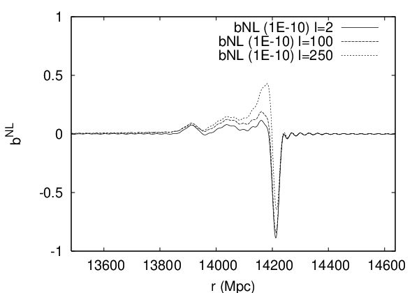
The functions $b_{l}^{NL}(r)$ and $b_{l}^{CI}(r)$ are evaluated using CMBFAST or related software Seljak and Zaldarriaga 1996. Some care has to be exercised in the evaluation of $b_{l}^{NL}(r)$ . It is important that the time evolution of the density perturbations in CMBFAST starts early in order to catch the large $k$ behaviour of the transfer function correctly. The function, $b_{l}^{NL}(r)$ has a large spike not far from $r=r_{*}$ , where

r_{*}=c\int_{t_{d}}^{t_{0}}{a(t_{0})\over a(t)}dt

(22)

is the speed of light times the conformal time difference between decoupling $t_{d}$ and the present $t_{0}$ . This is shown in figure 1. The resolution in $r$ has to be very high to capture this accurately, but this incurs a large time penalty when evaluating the angle averaged bispectrum for many different values of $l$ . We get around this problem by evaluating $b_{l}^{NL}(r)$ with a high resolution (3200 values of $r$ in the range $r_{*}\pm r_{d}$ ) and then averaging to produce a function $\bar{b}_{l}^{NL}(r)$ with a lower resolution. The integral over $r$ can be obtained accurately using $\bar{b}_{l}^{NL}(r)$ because the other terms in the integrand vary comparatively slowly with $r$ . More sophisticated methods of reducing the number of points in the $r$ integral are described in ref Smith and Zaldarriaga 2006

Refer to caption — Figure 1: The function $b_{l}^{NL}(r)$ is plotted as a function of $r$ in Mpc for $l=2$ , $l=100$ and $l=250$ . The cosmological model is the WMAP $\Lambda$ CDM plus $n=1$ model, which has $\Omega_{\Lambda}=0.788$ , $\Omega_{m}=0.212$ and $h=0.778$ . With these parameters, $r_{*}=1.41$ Gpc and $r_{d}=323$ Mpc.

II.2 Non-local models

The second model which we consider in detail is the model with $l=n=1$ , which we will denote by the label ‘WI’. The coefficients $c(l_{1}^{\prime}l_{2}^{\prime}1;l_{1}l_{2}l_{3})$ can be found using explicit formulae for the $6j$ symbols, given in ref Brink and Satchler 1993, for example. They can be expressed conveniently in terms of Edmond’s angle $\theta$ , defined by

\cos\theta=2{l_{1}(l_{1}+1)+l_{2}(l_{2}+1)-l_{3}(l_{3}+1)\over(2l_{1}+1)(2l_{2}+1)}

(23)

This angle is an interior angle of the simplex with sides corresponding to the entries in the $6j$ symbol. The non-vanishing coefficients are given by

	$\displaystyle{c(l_{1}\pm 1,l_{2}\pm 1,1;l_{1},l_{2},l_{3})\over c(l_{1}l_{2}0;l_{1}l_{2}l_{3})}$	$\displaystyle=$	$\displaystyle-{1\over 4}\left(\cos\theta+1\pm{1\over 2l_{1}+1}\pm{1\over 2l_{2}+1}+{1\over(2l_{1}+1)(2l_{2}+1)}\right)$		(24)
	$\displaystyle{c(l_{1}\pm 1,l_{2}\mp 1,1;l_{1},l_{2},l_{3})\over c(l_{1}l_{2}0;l_{1}l_{2}l_{3})}$	$\displaystyle=$	$\displaystyle-{1\over 4}\left(\cos\theta-1\mp{1\over 2l_{1}+1}\pm{1\over 2l_{2}+1}+{1\over(2l_{1}+1)(2l_{2}+1)}\right).$		(25)

The terms depending on $r$ can be simplified by using Bessel function identities,

$\displaystyle b^{1}_{ll+1}$	$\displaystyle=$	$\displaystyle{l\over r}b_{l}^{CI}(r)-b_{l}^{CI\prime}(r)$	(26)
$\displaystyle b^{1}_{ll-1}$	$\displaystyle=$	$\displaystyle{l+1\over r}b_{l}^{CI}(r)+b_{l}^{CI\prime}(r)$	(27)
$\displaystyle b^{-1}_{ll+1}$	$\displaystyle=$	$\displaystyle{l\over r}b_{l}^{WI}(r)-b_{l}^{WI\prime}(r)$	(28)
$\displaystyle b^{-1}_{ll-1}$	$\displaystyle=$	$\displaystyle{l+1\over r}b_{l}^{WI}(r)+b_{l}^{WI\prime}(r),$	(29)

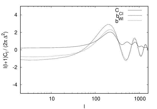
where the prime denotes a derivative with respect to $r$ and $b_{l}^{CI}(r)$ is given in eq. (21). We have introduced a new function $b_{l}^{WI}(r)$ , defined by

b_{l}^{WI}(r)={2\over\pi}\int_{0}^{\infty}dk\,P_{\zeta}(k)g_{l}(k)j_{l}(kr).

(30)

This is plotted in figure 2, together with the angular power spectrum $C_{l}$ , defined by,

C_{l}={2\over\pi}\int\,dk\,k^{2}\,P_{\zeta}(k)\,g_{l}(k)^{2}.

(31)

The angle-averaged bispectrum $B^{WI}_{l_{1}l_{1}l_{3}}$ is given by substituting the above functions into eq. (14),

	$\displaystyle B^{WI}_{l_{1}l_{1}l_{3}}$	$\displaystyle=$	$\displaystyle-\sum_{\rm perm}c(l_{1}l_{2}0;l_{1}l_{2}l_{3})\times$		(32)
			$\displaystyle\int_{0}^{\infty}\,dr\left(\left(l_{1}+{1\over 2}\right)\left(l_{2}+{1\over 2}\right)b_{l_{1}}^{CI}(r)b_{l_{2}}^{WI}(r)\cos\theta+b_{l_{1}}^{CI\prime}(r)b_{l_{2}}^{WI\prime}(r)r^{2}\right)b^{NL}_{l_{3}}(r),$		(32)

where $c(l_{1}l_{2}0;l_{1}l_{2}l_{3})$ is defined in eq. (19), $b^{NL}_{l}(r)$ is defined in eq (16) and $b_{l}^{CI}(r)$ in eq. (21). The radial functions and their derivatives can be evaluated using CMBFAST.

III Model testing

We shall use Maximum likelyhood methods methods to consider the sensitivity of ‘ideal’ experiments for detecting the non-local model of the bispectrum which we introduced in the previous section, and we shall consider how well this model can be distinguished from the local model. For our purposes, an ideal experiment is one in which there is no noise in the detector and no secondary sources of non-gaussianity.

For a single model, the log-likelyhood function $-\chi^{2}(B^{\rm obs}_{l_{1}l_{2}l_{3}},f)$ is a function of the nongaussianity parameter $f$ for a set of observations $B^{\rm obs}_{l_{1}l_{2}l_{3}}$ . For an ideal experiment, we take the simple anzatz

\chi^{2}={1\over 6}\sum_{l_{1}l_{2}l_{3}}{(B^{\rm obs}_{l_{1}l_{2}l_{3}}-fB_{l_{1}l_{2}l_{3}})^{2}\over C_{l_{1}}C_{l_{2}}C_{l_{3}}},

(33)

where $C_{l}$ is the angular power spectrum and $C_{l_{1}}C_{l_{2}}C_{l_{3}}$ is the theoretical variance of the bispectrum when the non-gaussianity is small. The sumations extend to a maximum $l$ value $l_{max}$ which represents the limiting resolution of the experiment.

This form of likelyhood function is associated with an estimator

\hat{f}={1\over 6F}\sum_{l_{1}l_{2}l_{3}}{B^{\rm obs}_{l_{1}l_{2}l_{3}}B_{l_{1}l_{2}l_{3}}\over C_{l_{1}}C_{l_{2}}C_{l_{3}}}

(34)

where the normalisation factor $F$ is the Fisher information,

F={1\over 6}\sum_{l_{1}l_{2}l_{3}}{(B_{l_{1}l_{2}l_{3}})^{2}\over C_{l_{1}}C_{l_{2}}C_{l_{3}}}.

(35)

For an ideal experiment, the mean of $\hat{f}$ is the value of the parameter $f$ and the variance of $\hat{f}$ is $F^{-1}$ .

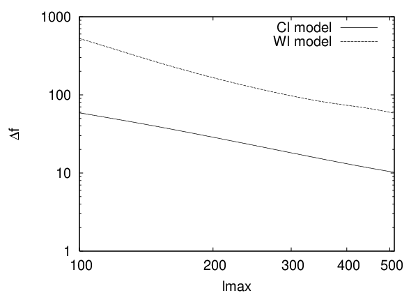
The standard deviation $\Delta f=F^{-1/2}$ has been plotted in figure 3, using the values of $B_{l_{1}l_{2}l_{3}}$ discussed in the previous section. The WMAP $\Lambda$ CDM plus $n=1$ cosmological model has been used to define the cosmological parameters. The standard deviation for the local model is in good agreement with previous calculations, even when they use different cosmological parameters Creminelli et al. 2006.

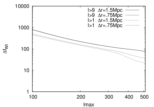
The calculation of the standard deviation for the WI model with $l_{max}=512$ takes about 30 minutes on a 2GHz Intel Core Duo processor. The time is taken up by the high resolution used to evaluate the radial integrals when we get to values of $l\sim 400$ . The high resolution is needed mostly for the ‘squeezed triangles’, where one value of $l$ in the summand is far smaller than the other two. This fact shows up clearly in figure 4, where the plots show that the dependence on resolution dissappears when low multipoles have been omitted from the sum. Our resolution is adequate for the maximum value $l=300$ in the next section. For the Planck experiment we would need to push the limit up to $l=2000$ or so. In this higher range, an increase in the standard deviation arising from dropping low multipoles may well be acceptable as a trade-off for having to perform the calculations with many values of $r$ . For example, the resolution used here is already sufficient to obtain the variance of the estimator for the WI model from modes in the range $9<l<1800$ , and it comes out to be $\Delta f_{WI}=15.9$ . This is an upper bound on the variance of the estimator which uses all of the modes $1<l<1800$ .

The observations can also be used to distinguish between two different models $B^{i}_{l_{1}l_{2}l_{3}}$ , $i=1,2,\dots$ . The Fisher information is now a matrix,

F_{ij}={1\over 6}\sum_{l_{1}l_{2}l_{3}}{B^{i}_{l_{1}l_{2}l_{3}}B^{j}_{l_{1}l_{2}l_{3}}\over C_{l_{1}}C_{l_{2}}C_{l_{3}}}.

(36)

The separability of two different models is associated with a low value for the correlation

r=-{F_{12}\over\sqrt{F_{11}F_{22}}}.

(37)

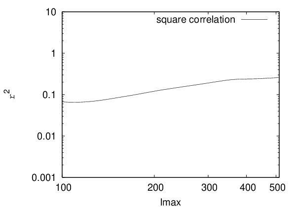
(This quantity was called the ‘cosine between two distributions’ in ref. Babich et al. 2004). If two bispectra have good separability, then the failure to detect any non-gaussianity for one bispectrum does not rule out the possibility of detection of non-gaussianity in the other bispectrum. The square of the correlation for the $CI$ and $WI$ models has been plotted in figure 5. At $l=300$ , the square of the correlation is about 10%, which is quite low but not low enough to separate the two models definitively using this statistic.

IV Non-gaussianity tests on CMB data

The estimator for the non-gaussianity of model $i$ in an ideal experiment was given in the previous section,

\hat{f}^{\rm ideal}_{i}={1\over 6F_{ii}}\sum_{l_{1}l_{2}l_{3}}{B^{\rm obs}_{l_{1}l_{2}l_{3}}B^{i}_{l_{1}l_{2}l_{3}}\over C_{l_{1}}C_{l_{2}}C_{l_{3}}},

(38)

where the observed angle-averaged bispectrum is related to the spherical harmonic coefficients by

B^{\rm obs}_{l_{1}l_{2}l_{3}}=\sum_{m_{1}m_{2}m_{2}}\pmatrix{l_{1}&l_{2}&l_{3}\cr m_{1}&m_{2}&m_{3}}a_{l_{1}m_{1}}a_{l_{2}m_{2}}a_{l_{3}m_{3}}.

(39)

We can make use use the fact that the theoretical bispectrum eq. (20) or eq. (32) consist of a small number of terms which factorise to devise an efficient method for evaluating the estimators based on ref. Komatsu et al. 2005.

The Wigner $3j$ symbol is first replaced by the integral

\pmatrix{l_{1}&l_{2}&l_{3}\cr m_{1}&m_{2}&m_{3}}=c(l_{1}l_{2}0;l_{1}l_{2}l_{3})^{-1}\int d^{2}\hat{\bf n}\,Y_{l_{1}m_{1}}(\hat{\bf n})Y_{l_{2}m_{2}}(\hat{\bf n})Y_{l_{3}m_{3}}(\hat{\bf n}),

(40)

where $c(l_{1}l_{2}0;l_{1}l_{2}l_{3})$ is defined in eq. (19), to give

\hat{f}^{\rm ideal}_{i}={1\over 6F_{ii}}\sum_{l_{i}m_{i}}c(l_{1}l_{2}0;l_{1}l_{2}l_{3})^{-1}\int d^{2}\hat{\bf n}\prod_{i=1}^{3}\left(a_{l_{i}m_{i}}Y_{l_{i}m_{i}}(\hat{\bf n})\right){B^{i}_{l_{1}l_{2}l_{3}}\over C_{l_{1}}C_{l_{2}}C_{l_{3}}}.

(41)

Now we define a radial sequence of filtered sky-maps $\sigma(r,\hat{\bf n})$ by

$\displaystyle\sigma_{CI}(r,\hat{\bf n})$	$\displaystyle=$	$\displaystyle\sum_{l,m}{b_{l}^{CI}(r)\over C_{l}}a_{lm}Y_{lm}(\hat{\bf n})$	(42)
$\displaystyle\sigma_{WI}(r,\hat{\bf n})$	$\displaystyle=$	$\displaystyle\sum_{l,m}{b_{l}^{WI}(r)\over C_{l}}a_{lm}Y_{lm}(\hat{\bf n})$	(43)
$\displaystyle\sigma_{NL}(r,\hat{\bf n})$	$\displaystyle=$	$\displaystyle\sum_{l,m}{b_{l}^{NL}(r)\over C_{l}}a_{lm}Y_{lm}(\hat{\bf n}).$	(44)

For the local model, $B^{CI}_{l_{1}l_{2}l_{3}}$ is given by eq. (20). After interchanging the sum and the integrals in eq. (41),

\hat{f}^{\rm ideal}_{CI}={1\over F_{CI}}\int d^{2}\hat{\bf n}\,r^{2}dr\,\sigma_{CI}\sigma_{CI}\sigma_{NL}

(45)

This can be evaluated easily with the HEALPix ¹¹ 1 See the HEALPix website http://www.eso.org/science/healpix software package for analysing CMB data.

The second model has angle averaged bispectrum given by eq. (32). The $l(l+1)$ terms in Edmond’s angle $\theta$ (23) can be replaced by the angular Laplacian $D^{2}$ , defined by

D^{2}Y_{lm}(\hat{\bf n})=-l(l+1)Y_{lm}(\hat{\bf n}).

(46)

The estimator becomes

\hat{f}^{\rm ideal}_{WI}={1\over 2F_{WI}}\int d^{2}\hat{\bf n}\,dr\,\left\{(D^{2}\sigma_{CI})\sigma_{WI}\sigma_{NL}+\sigma_{CI}(D^{2}\sigma_{WI})\sigma_{NL}-\sigma_{CI}\sigma_{WI}(D^{2}\sigma_{NL})-2\sigma^{\prime}_{CI}\sigma^{\prime}_{WI}\sigma_{NL}r^{2}\right\}.

(47)

We can regard this as a volume integral and use the divergence theorem,

\hat{f}^{\rm ideal}_{WI}=-{1\over F_{WI}}\int d^{3}x\,(\nabla\sigma_{CI})\cdot(\nabla\sigma_{WI})\sigma_{NL},

(48)

where $\nabla$ is the three dimensional gradient operator. This expression can be evaluated at high speed using the subroutines for handling angular derivatives of CMB data in the HEALPix software package.

IV.1 Real experiments

Galactic and extragalactic sources contaminate the cosmological microwave signal and have to be masked out, leaving us with a set of spherical coefficients $a_{lm}$ of the masked sky. The statistical properties of these coefficients are affected by the masking procedure. An important change appears in the theoretical covariance matrix

C_{l_{1}m_{1}l_{2}m_{2}}=\langle a_{l_{1}m_{1}}a_{l_{2}m_{2}}\rangle,

(49)

which is no longer diagonal. Detector noise is also an important consideration. The detector noise is not uniform over the sky and the noise in the microwave intensity has a non-trivial covariance matrix.

Creminelli et al. Creminelli et al. 2006 have introduced an improved estimator which should be close to optimal for the CMB observations. Their estimator

\hat{f}_{i}=\hat{f}_{i}^{\rm ideal}+\hat{f}_{i}^{\rm lin},

(50)

where the linear piece

\hat{f}_{i}^{\rm lin}=-{1\over 2N}\sum_{l_{1}l_{2}l_{3}}{B^{i}_{l_{1}l_{2}l_{3}}\over C_{l_{1}}C_{l_{2}}C_{l_{3}}}C_{l_{1}m_{1}l_{2}m_{2}}a_{l_{3}m_{3}}.

(51)

The normalisation factor $N=F_{ii}f_{\rm sky}$ , where $f_{\rm sky}$ is the fraction of the sky which remains after the mask is applied.

The linear part of the estimator can be expressed in terms of filtered maps by following the same steps as in the beginning of this section. We shall concentrate here on the effects of the mask. To a reasonable approximation, it can be shown that

\sum_{l_{1}l_{2}m_{1}m_{2}}b_{l_{1}}b_{l_{2}}Y_{l_{1}m_{1}}(\hat{\bf n})C_{l_{1}m_{1}l_{2}m_{2}}Y_{l_{1}m_{1}}(\hat{\bf n})\approx M(\hat{\bf n})\sum_{l}{2l+1\over 4\pi}b_{l}^{2}C_{l}

(52)

where $b_{l}$ is any slowly varying function of $l$ and the mask function $M(\hat{\bf n})=0$ in the region being masked out and $1$ otherwise. The details are given in the appendix. Using this approximation, the linear parts of the estimators become

	$\displaystyle\hat{f}^{\rm lin}_{CI}$	$\displaystyle=$	$\displaystyle-{1\over N_{CI}}\int d^{2}\hat{\bf n}\,r^{2}dr\,M\left(2S_{CINL}\sigma_{CI}+S_{CICI}\sigma_{NL}\right)$		(53)
	$\displaystyle\hat{f}^{\rm lin}_{WI}$	$\displaystyle=$	$\displaystyle{1\over N_{WI}}\int d^{2}\hat{\bf n}\,r^{2}dr\,M\left(\tilde{S}_{CIWI}\sigma_{NL}+S^{(2)}_{CIWI}\sigma_{NL}+S^{(1)}_{CINL}\sigma^{\prime}_{WI}+S^{(1)}_{WINL}\sigma^{\prime}_{CI}\right)$		(54)

where the radial functions $S_{AB}(r)$ , $A$ , $B=CI$ , $WI$ or $NL$ , are defined by

$\displaystyle S_{AB}(r)$	$\displaystyle=$	$\displaystyle\sum_{l}\,{2l+1\over 4\pi}{b_{l}^{A}(r)b_{l}^{B}(r)\over C_{l}}$	(55)
$\displaystyle\tilde{S}_{AB}(r)$	$\displaystyle=$	$\displaystyle\sum_{l}\,l(l+1){2l+1\over 4\pi}{b_{l}^{A}(r)b_{l}^{B}(r)\over C_{l}}$	(56)
$\displaystyle S^{(1)}_{AB}(r)$	$\displaystyle=$	$\displaystyle\sum_{l}\,{2l+1\over 4\pi}{b_{l}^{A}(r)^{\prime}b_{l}^{B}(r)\over C_{l}}$	(57)
$\displaystyle S^{(2)}_{AB}(r)$	$\displaystyle=$	$\displaystyle\sum_{l}\,{2l+1\over 4\pi}{b_{l}^{A}(r)^{\prime}b_{l}^{B}(r)^{\prime}\over C_{l}}.$	(58)

The linear parts should be combined with the other terms (45) and (48).

Crenelli et al. Creminelli et al. 2006 have argued that since the contributions from the linear terms depend on angular averages of the filtered maps, they can be reduced in size by arranging that the average value of the data outside the mask is zero. However, we have found that the contributions from the linear terms are important and they need to be included.

IV.2 WMAP data

We shall consider the non-gaussianity estimators for the 3-year data which has been made available by the WMAP collaboration. The angular resolution of this data should allow values of $l$ up to 300-400, but we have chosen to take the maximum value of $l$ for which detector noise can be neglected, and this is around $l=300$ . We have used 800 values of $r$ in the range $13750{\rm Mpc}<r<14350{\rm Mpc}$ and 200 values of $r$ for $8750{\rm Mpc}<r<13750{\rm Mpc}$ . (Values of $r$ outside this range appear to make very little change to the estimators).

The values of the estimators and the variance of the ideal experiment are shown in table 1. The rms values of the estimators for a set of randomly generated gaussian maps have been used to check that the linear term in the estimator removes the effects of the mask without biasing the estimator. Leaving out the linear term gives a spurious signal.

The results for $f_{CI}$ can be expressed as a constraint on the more commonly used parameter $f_{NL}$ , where $f_{CI}=0.6f_{NL}$ ,

-26<f_{NL}<109\hbox{~~~~~at 95\% C.L.}

(59)

which we should stress ignores detector noise. This is consistent with the results published by the WMAP collaboration given the fact that the detector noise increases the standard deviation of the estimator by 10-20% Komatsu et al. 2003. The results for the WI model are

-375<f_{WI}<36.8\hbox{~~~~~at 95\% C.L.}

(60)

Although there is no evidence for a signal, it may be worth pointing out that $f_{WI}<0$ at 94% C.L., and this would be in agreement with the predictions of the warm inflationary model Moss and Xiong 2007.

Map	Mask	$f_{\rm sky}$	$l$	$f_{CI}$	$\Delta f_{CI}$	$f_{WI}$	$\Delta f_{WI}$
W	kp0	0.765	300	24.9	20.5	-169	105
V	kp0	0.765	300	33.7	20.5	-174	105
R	kp0	0.765	300	-0.712	13.4	3.09	89.2

Table 1: Values of the estimator (with the linear correction) and variance for a selection of 3-year WMAP datasets and masks. The frequency bands are denoted by

W

and

V

and the maps are ‘foreground reduced’. The row labelled

R

gives the average and rms average of the estimator over 20 randomly generated gaussian maps. The deviation

\Delta f

in rows

W

and

V

is the deviation for an ideal experiment scaled by the unmasked fraction of the sky

f_{\rm sky}

V Conclusion

We have compared two different bispectra which represent the non-gaussianity in the CMB produced by two different types of inflation. The first bispectrum (CI) is of the local type, which can result from a curvaton field and the second (WI) was modelled on a result deduced from the theory of warm inflation. In the second example we found a new, simple form for the estimator used to quantify the amount of non-gaussianity present in the CMB data.

The WI bispectrum demands accurate handling of the numerical integrations and also careful consideration of the effects introduced by masking out part of the sky. We have introduced a binning technique to improve the accuracy of the integrations and used an improved estimator to deal with the masked data.

The variance of the estimator for the WI nongaussianity in an ideal experiment using modes up to $l=500$ is plotted in figure 3. Beyond $l=500$ , we would have to improve the resolution in the integrations, remove some of the lower $l$ modes or adopt an alternative computational strategy Smith and Zaldarriaga 2006. For example, using modes in the range $9<l<1800$ sets an upper bound on the deviation of $\Delta f_{WI}<15.9$ .

When applied to the WMAP 3-year data we reproduce similar results to previous work for the CI bispectrum. So far there is no evidence for the WI bispectrum, and the limits are

-375<f_{WI}<36.8\hbox{~~~~~at 95\% C.L.}

(61)

According to the calculation in ref. Moss and Xiong 2007, the strong regime of warm inflation leads to the WI bispectrum with

f_{WI}\approx-18\ln\left(1+{r\over 14}\right)

(62)

where $r$ is a large parameter. It is possible to predict the probability of a $2\sigma$ signal from the Planck satellite for this model. Using $\Delta f_{WI}<15.9$ , a $2\sigma$ signal would be obtained with better than 95% probability if $r>65$ .

Appendix A Some properties of masked data

Consider the situation where we expect a gaussian signal $\sigma(\hat{\bf n})$ but due to unwanted background sources we mask out an area of the sky ${\cal M}$ . The masked spherical harmonic coefficients are

a_{lm}=\int d^{2}\hat{\bf n}\,M(\hat{\bf n})\sigma(\hat{\bf n})Y^{*}_{lm}(\hat{\bf n})

(63)

where $M(\hat{\bf n})=0$ for $\hat{\bf n}\in{\cal M}$ and $M(\hat{\bf n})=1$ otherwise. The covariance matrix of the masked coefficients is defined by

C_{l_{1}m_{1}l_{2}m_{2}}=\langle a_{l_{1}m_{1}}a_{l_{2}m_{2}}\rangle.

(64)

This can be expressed in terms of the angular power spectrum $C_{l}$ of the full-sky coefficients,

C_{l_{1}m_{1}l_{2}m_{2}}=\sum_{lm}\,C_{l}\,\int d^{2}\hat{\bf n}_{1}d^{2}\hat{\bf n}_{2}M(\hat{\bf n}_{1})M(\hat{\bf n}_{2})Y^{*}_{l_{1}m_{1}}(\hat{\bf n}_{1})Y^{*}_{l_{2}m_{2}}(\hat{\bf n}_{2})Y_{lm}(\hat{\bf n}_{1})Y_{lm}(\hat{\bf n}_{2}).

(65)

The main objective of this appendix is to approximate the sum

F(\hat{\bf n})=\sum_{l_{1}l_{2}m_{1}m_{2}}b_{l_{1}}b_{l_{2}}Y_{l_{1}m_{1}}(\hat{\bf n})C_{l_{1}m_{1}l_{2}m_{2}}Y_{l_{1}m_{1}}(\hat{\bf n}),

(66)

where $b_{l}$ is a slowly varying function of $l$ . Using eq. (65),

F(\hat{\bf n})=\int d^{2}\hat{\bf n}_{1}d^{2}\hat{\bf n}_{2}M(\hat{\bf n}_{1})M(\hat{\bf n}_{2})K(\hat{\bf n},\hat{\bf n}_{1})K(\hat{\bf n},\hat{\bf n}_{2})\sum_{lm}C_{l}Y_{lm}(\hat{\bf n}_{1})Y_{lm}(\hat{\bf n}_{2})

(67)

where the kernel $K(\hat{\bf n},\hat{\bf n}^{\prime})$ is given by

K(\hat{\bf n},\hat{\bf n}^{\prime})=\sum_{lm}b_{l}Y_{lm}(\hat{\bf n})Y_{lm}(\hat{\bf n}^{\prime}).

(68)

The next step is to clarify the sense in which the $b_{l}$ are slowly varying. Introduce a new function $b(t)$ by

b_{l}=\int_{0}^{\infty}e^{-l(l+1)t}b(t)dt.

(69)

We say that the $b_{l}$ are slowly varying if $b(t)=0$ for $t>\mu$ , where $\mu$ is a small parameter. For primordial fluctuations, the scale of variation of the $b_{l}$ ’s is set by the acoustic oscillations, and $\mu$ is a small parameter determined by the conformal time at the last scattering surface. (In reallity $b(t)$ will not vanish for $t>\mu$ , but it must be relatively small in view of the smoothness of the plots of the $b_{l}$ ’s).

The kernel $K(\hat{\bf n},\hat{\bf n}^{\prime})$ is related to the fundamental solution to the heat equation on a unit sphere $K(\hat{\bf n},\hat{\bf n}^{\prime},t)$ by

K(\hat{\bf n},\hat{\bf n}^{\prime})=\int_{0}^{\infty}dt\,K(\hat{\bf n},\hat{\bf n}^{\prime},t)b(t).

(70)

For small time, we can use the asymptotic expansion

K(\hat{\bf n},\hat{\bf n}^{\prime},t)={1\over 4\pi t}e^{-d(\hat{\bf n},\hat{\bf n}^{\prime})^{2}/4t}\left(1+O(t^{2})\right),

(71)

where $d(\hat{\bf n},\hat{\bf n}^{\prime})$ is the great circle distance between $\hat{\bf n}$ and $\hat{\bf n}^{\prime}$ , to get an upper bound,

|K(\hat{\bf n},\hat{\bf n}^{\prime})|\leq K_{0}e^{-d(\hat{\bf n},\hat{\bf n}^{\prime})^{2}/4\eta}

(72)

where $K_{0}=\sum_{l}(2l+1)b_{l}$ and $O(\eta^{2})$ corrections are dropped.

If the mask is empty, then the orthogonality property of the spherical harmonics can be used to show that the function $F$ takes a constant value $S$ , where

S=\sum_{l}\,{2l+1\over 4\pi}b_{l}^{2}C_{l}.

(73)

Now use eq. (67) to calculate the difference

|F(\hat{\bf n})-SM(\hat{\bf n})|\leq\int d^{2}\hat{\bf n}_{1}d^{2}\hat{\bf n}_{2}\left|(M(\hat{\bf n}_{1})M(\hat{\bf n}_{2})-M(\hat{\bf n}))K(\hat{\bf n},\hat{\bf n}_{1})K(\hat{\bf n},\hat{\bf n}_{2})\sum_{lm}C_{l}Y_{lm}(\hat{\bf n}_{1})Y_{lm}(\hat{\bf n}_{2})\right|

(74)

We have a bound (72) on the kernel and we can bound the final sum by a constant $C$ ,

\left|\sum_{lm}C_{l}Y_{lm}(\hat{\bf n}_{1})Y_{lm}(\hat{\bf n}_{2})\right|\leq C=\sum_{l}{4\pi\over 2l+1}C_{l}.

(75)

Consider the case where $\hat{\bf n}\in{\cal M}$ , which forces the integrand into the rest of the sky $\bar{\cal M}$ ,

|F(\hat{\bf n})-SM(\hat{\bf n})|\leq CK_{0}^{2}\,\left(\int_{\bar{\cal M}}d^{2}\hat{\bf n}^{\prime}e^{-d(\hat{\bf n},\hat{\bf n}^{\prime})^{2}/4\eta}\right)^{2}

(76)

There is an assymptotic expansion for the integral for small $\eta$ obtained by setting $\hat{\bf n}^{\prime}=\hat{\bf n}_{c}+\epsilon$ , where $\hat{\bf n}_{c}$ is the closest point on the edge of the mask to $\hat{\bf n}$ . The result is that

|F(\hat{\bf n})-SM(\hat{\bf n})|\leq CK_{0}^{2}\pi(2\eta)^{3}e^{-d(\hat{\bf n},\hat{\bf n}_{c})^{2}/2\eta}.

(77)

A similar argument applies when $\hat{\bf n}\in\bar{\cal M}$ . The approximation $F\approx SM(\hat{\bf n})$ holds as long as the point on the sky does not approach too closely the edge of the mask where $d(\hat{\bf n},\hat{\bf n}_{c})=0$ .

References

Falk et al. (1993) T. Falk, R. Rangarajan, and M. Srednicki, Astrophys. J. 403, L1 (1993), eprint astro-ph/9208001.
Gangui et al. (1994) A. Gangui, F. Lucchin, S. Matarrese, and S. Mollerach, Astrophys. J. 430, 447 (1994), eprint astro-ph/9312033.
Acquaviva et al. (2003) V. Acquaviva, N. Bartolo, S. Matarrese, and A. Riotto, Nucl. Phys. B667, 119 (2003), eprint astro-ph/0209156.
Komatsu and Spergel (2001) E. Komatsu and D. N. Spergel, Phys. Rev. D63, 063002 (2001), eprint astro-ph/0005036.
Munshi et al. (1995) D. Munshi, T. Souradeep, and A. A. Starobinsky, Astrophys. J. 454, 552 (1995), eprint astro-ph/9501100.
Pyne and Carroll (1996) T. Pyne and S. M. Carroll, Phys. Rev. D53, 2920 (1996), eprint astro-ph/9510041.
Lyth et al. (2005) D. H. Lyth, K. A. Malik, and M. Sasaki, JCAP 0505, 004 (2005), eprint astro-ph/0411220.
Sasaki et al. (2006) M. Sasaki, J. Valiviita, and D. Wands, Phys. Rev. D74, 103003 (2006), eprint astro-ph/0607627.
Dvali et al. (2004) G. Dvali, A. Gruzinov, and M. Zaldarriaga, Phys. Rev. D69, 083505 (2004), eprint astro-ph/0305548.
Moss and Xiong (2007) I. G. Moss and C. Xiong, JCAP 0704, 007 (2007), eprint astro-ph/0701302.
Bardeen et al. (1983) J. M. Bardeen, P. J. Steinnhart, and M. S. Turner, Phys. Rev. D 28, 679 (1983).
Lyth and Rodriguez (2005) D. H. Lyth and Y. Rodriguez, Phys. Rev. Lett. 95, 121302 (2005), eprint astro-ph/0504045.
Spergel et al. (2006) D. N. Spergel et al. (2006), eprint astro-ph/0603449.
Moss (1985) I. G. Moss, Phys. lett. 154B, 120 (1985).
Berera (1995) A. Berera, Phys. Rev. lett. 75, 3218 (1995).
Liguori et al. (2006) M. Liguori, F. K. Hansen, E. Komatsu, S. Matarrese, and A. Riotto, Phys. Rev. D73, 043505 (2006), eprint astro-ph/0509098.
Smith and Zaldarriaga (2006) K. M. Smith and M. Zaldarriaga (2006), eprint astro-ph/0612571.
Creminelli et al. (2006) P. Creminelli, A. Nicolis, L. Senatore, M. Tegmark, and M. Zaldarriaga, JCAP 0605, 004 (2006), eprint astro-ph/0509029.
Creminelli (2003) P. Creminelli, JCAP 0310, 003 (2003), eprint astro-ph/0306122.
Seljak and Zaldarriaga (1996) U. Seljak and M. Zaldarriaga, Astrophys. J. 469, 437 (1996), eprint astro-ph/9603033.
Brink and Satchler (1993) D. M. Brink and G. R. Satchler, Angular Momentum (Oxford Science Publications, 1993), 3rd ed., appendix II.
Komatsu (2002) E. Komatsu (2002), eprint astro-ph/0206039.
Babich et al. (2004) D. Babich, P. Creminelli, and M. Zaldarriaga, JCAP 0408, 009 (2004), eprint astro-ph/0405356.
Komatsu et al. (2005) E. Komatsu, D. N. Spergel, and B. D. Wandelt, Astrophys. J. 634, 14 (2005), eprint astro-ph/0305189.
Komatsu et al. (2003) E. Komatsu et al. (WMAP), Astrophys. J. Suppl. 148, 119 (2003), eprint astro-ph/0302223.