Analysis of the accuracy and convergence
of equation-free projection to a slow manifold
May 14, 2007
A. Zagaris1,2, C. W. Gear3,4, T. J. Kaper5, I. G. Kevrekidis3,6
Department of Mathematics, University of Amsterdam, Amsterdam, The Netherlands.
Modeling, Analysis and Simulation, Centrum voor Wiskunde en Informatica, Amsterdam, The Netherlands.
Department of Chemical Engineering, Princeton University, Princeton, NJ 08544;
NEC Laboratories USA, retired;
Department of Mathematics and Center for BioDynamics, Boston University, Boston, MA 02215;
Program in Applied and Computational Mathematics, Princeton University, Princeton, NJ 08544;
Abstract
In [C. W. Gear, T. J. Kaper, I. G. Kevrekidis, and A. Zagaris, Projecting to a Slow Manifold: Singularly Perturbed Systems and Legacy Codes, SIAM J. Appl. Dyn. Syst. 4 (2005) 711–732], we developed a class of iterative algorithms within the context of equation-free methods to approximate low-dimensional, attracting, slow manifolds in systems of differential equations with multiple time scales. For user-specified values of a finite number of the observables, the th member of the class of algorithms () finds iteratively an approximation of the appropriate zero of the st time derivative of the remaining variables and uses this root to approximate the location of the point on the slow manifold corresponding to these values of the observables. This article is the first of two articles in which the accuracy and convergence of the iterative algorithms are analyzed. Here, we work directly with explicit fast–slow systems, in which there is an explicit small parameter, , measuring the separation of time scales. We show that, for each , the fixed point of the iterative algorithm approximates the slow manifold up to and including terms of . Moreover, for each , we identify explicitly the conditions under which the th iterative algorithm converges to this fixed point. Finally, we show that when the iteration is unstable (or converges slowly) it may be stabilized (or its convergence may be accelerated) by application of the Recursive Projection Method. Alternatively, the Newton–Krylov Generalized Minimal Residual Method may be used. In the subsequent article, we will consider the accuracy and convergence of the iterative algorithms for a broader class of systems—in which there need not be an explicit small parameter—to which the algorithms also apply.
1 Introduction
The long-term dynamics of many complex chemical, physical, and biological systems simplify when a low-dimensional, attracting, invariant slow manifold is present. Such a slow manifold attracts all nearby initial data exponentially, and the reduced dynamics on it govern the long term evolution of the full system. More specifically, a slow manifold is parametrized by observables which are typically slow variables or functions of variables. All nearby system trajectories decompose naturally into a fast component that contracts exponentially toward the slow manifold and a slow component which obeys the reduced system dynamics on the manifold. In this sense, the fast variables become slaved to the observables, and knowledge of the slow manifold and of the reduced dynamics on it suffices to determine the full long-term system dynamics.
The identification and approximation of slow manifolds is usually achieved by employing a reduction method. We briefly list a number of these: Intrinsic Low Dimensional Manifold (ILDM), Computational Singular Perturbation (CSP), Method of Invariant Manifold (MIM), Approximate Inertial Manifold approaches, and Fraser-Roussel iteration, and we refer the reader to [4, 8] for a more extensive listing.
1.1 A class of iterative algorithms based on the zero-derivative principle
In [4], we developed a class of iterative algorithms to locate slow manifolds for systems of Ordinary Differential Equations (ODEs) of the form
where . We treated the variables as the observables (that is, as parametrizing the slow manifold we are interested in), and we assumed that there exists an dimensional, attracting, invariant, slow manifold , which is given locally by the graph of a function . However, we emphasize that we did not need explicit knowledge of which variables are fast and which are slow, only that the variables suffice to parametrize .
To leading order, the location of a slow manifold is obtained by setting , i.e., by solving for . Of course, the manifold defined by this equation is in general not an invariant slow manifold under the flow of the full system (1.1). This is only approximately true, since higher-order derivatives with respect to the (fast) time are, in general, large on it. If one requires that vanishes, then the solutions with initial conditions at the points defined by this condition depend only on the slow time to one order higher, as also remains bounded in the vicinity of this manifold. Similarly, demanding that successively higher-order time derivatives vanish, we obtain manifolds where all time derivatives of lower order remain bounded. The solutions with these initial conditions depend only on the slow time to successively higher order and thus approximate, also to successively higher order, solutions on the slow manifold. In other words, demanding that time derivatives of successively higher order vanish, we filter out the fast dynamics of the solutions to successively higher orders. In this manner, the approximation of the slow manifold is improved successively, as well. This idea may be traced back at least to the work of Kreiss [1, 11, 12], who studied systems with rapid oscillations (asymptotically large frequencies) and introduced the bounded derivative principle to find approximations of slow manifolds as the sets of points at which the derivatives are bounded (not large). The requirement here that the derivatives with respect to the (fast) time vanish is the analog for systems (1.1) with asymptotically stable slow manifolds. A similar idea was introduced independently by Lorenz in [13], where he used a simple functional iteration scheme to approximate the zero of the first derivative, then used the converged value of this scheme to initialize a similar scheme that approximates the zero of the second derivative, and so on until successive zeroes were found to be virtually identical. See also [3] and [6] for other works in which a similar condition is employed.
The elements of the class of iterative algorithms introduced in [4] are indexed by . The th algorithm is designed to locate, for any fixed value of the observable , an appropriate solution, , of the st derivative condition
| (1.4) |
Here, the time derivatives are evaluated along solutions of (1.1). In general, since condition (1.4) constitutes a system of nonlinear algebraic equations, the solution cannot be computed explicitly. Also, the explicit form of (1.1), and thus also an analytic formula for the st time derivative in Eq. (1.4), may be unavailable (e.g., in Equation-Free or legacy code applications). In this case, a numerical approximation for it has to be used. The -th algorithm in the class generates an approximation of , rather than itself, using either an analytic formula for the time derivative or a finite difference approximation for it. In either case, the approximation to is determined through an explicit functional iteration scheme, which we now introduce.
The algorithm is defined by the map
where , which we label as the iterative step size, is an arbitrary positive number whose magnitude we fix below for stability reasons. We initialize the iteration with some value and generate the sequence
The functional iteration is terminated when , for some and a prescribed tolerance . The output of this zeroth algorithm is the last member, , of the sequence .
Next, the algorithm is defined by the map ,
initialized with some value . It generates the sequence
and the functional iteration is terminated when , for some and for a prescribed tolerance . The output of this first algorithm is the last member, , of the sequence .
The algorithm with general is defined by the map ,
| (1.5) |
seeded with some value . It generates the sequence
Here also, one prescribes a tolerance and terminates the iteration procedure when for some . The output of this th algorithm is the last member of the sequence , denoted by .
As we show in this article, not only is the point of interest for each individual because it approximates , but the entire sequence is also of interest because it converges to with a suitably convergent sequence . Hence, the latter point can be approximated arbitrarily well by members of that sequence, and the class of algorithms may be used as an integrated sequence of algorithms in which the output of the th algorithm can be used to initialize the st algorithm. Of course, other initializations are also possible, and we have carried out the analysis here in a manner that is independent of which choice one makes.
This class of iterative algorithms was applied in [4] to three examples: the two-dimensional Michaelis–Menten mechanism for which the one-dimensional slow manifold can be computed analytically to arbitrary precision, a five-dimensional nonlinear system with an explicitly computable two-dimensional slow manifold, and a seven-dimensional hydrogen-oxygen system with quadratic nonlinearities for which the manifold is not known explicitly. In the context of these three examples, we found that, for all of the values of that we worked with, the -th algorithm converged at an exponential rate to a fixed point. Moreover, in the two examples where the slow manifold can be computed, we also found that, for each algorithm, this fixed point is very close to the actual point on the slow manifold. In addition to showing the -th algorithm converged for each that we worked with, we also showed that the class of algorithms may be used in the integrated manner stated above. The closeness of the approximation to improved as we increased the order of the algorithm used.
More recently, van Leemput et al. [16] employed the first () algorithm in the class to initialize Lattice Boltzmann Models (LBM) from sets of macroscopic data in a way that eliminates the stiff dynamics triggered by a bad initialization. They showed that the algorithm they derived converges unconditionally to a fixed point close to a slow manifold, and they used the algorithm to couple a LBM to a reaction-diffusion equation along the interface with good results [17].
Our motivation for introducing this class of iterative algorithms in [4] was two-fold. First, we wanted a method that can be implemented in the context of legacy codes. In other words, we wanted this reduction method to be implementable even when one has no explicit form for the components and of the vector field, but only a black-box integrator (timestepper). This feature renders the method “equation-free” [10] and makes its implementation possible in these settings. Second, it was essential for us that they preserve the user-specified value of the observables, say , at each iteration. In this way, the output of the algorithm is an approximation of the point on the manifold of that same value of the observables. Also, in this way, the ‘lifting’ step in projective integration of [5] is naturally facilitated.
It is worth noting that one really only needs to require that the time derivatives are sufficiently small, although we work with the zero-derivative condition (1.4) for definiteness.
1.2 Iterative algorithms based on the zero-derivative principle for explicit fast–slow systems
A central assumption that we made in [4] is that we work with systems (1.1) for which there exists a smooth and invertible coordinate change
| (1.6) |
where and , which puts the system (1.1) into the explicit fast–slow form
We emphasize that, in general, we have no knowledge whatsoever of the transformation that puts system (1.1) into an explicit fast–slow form. Here, and are smooth functions of their arguments, the manifold is transformed smoothly, and on the manifold (on which the dynamics reduce for ), see also [4].
Due to the above assumption, it turns out to be natural to split the analysis of the accuracy and convergence of the functional iteration into two parts. In the first part, which we present in this article, we work directly on systems that are already in explicit fast–slow form (1.2). In the context of these systems, the accuracy and convergence analysis may be carried out completely in terms of the small parameter . The system geometry – the slow manifold and the fast fibers transverse to – makes the convergence analysis especially transparent. Then, in the second part, we work with the more general systems (1.1). For these, the accuracy analysis proceeds along similar lines as that for this first part, with the same type of result as Theorem 2.1 below. However, the convergence analysis is considerably more involved than that for explicit fast–slow systems. For these general systems, one must analyze a series of different scenarios depending on the relative orientations of (i) the tangent space to , (ii) the tangent spaces to the fast fibers at their base points on , and (iii) the hyperplane of the observables . Moreover, all of the analysis must be carried out through the lens of the coordinate change (1.6) and its inverse, so that it is less transparent than it is in part one. Part two will be presented as a subsequent article.
As applied specifically to explicit fast–slow systems (1.2), the th iterative algorithm (1.5) is based on the st derivative condition,
| (1.10) |
In particular, for each and for any arbitrary, but fixed, value of the observable , one makes an initial guess for and uses the -th iterative algorithm to approximate the appropriate zero of this st derivative, where the end (converged) result of the iteration is the improved approximation of .
For each , the th iterative algorithm is defined by the map ,
| (1.11) |
where is an arbitrary positive number whose magnitude is for stability reasons. We seed with some value and generate the sequence
| (1.12) |
Here also, one prescribes a tolerance and terminates the iteration procedure when for some . The output of this th algorithm is the last member of the sequence , denoted by .
1.3 Statement of the main results
In this article, we first examine the -th iterative algorithm in which an analytical formula for the st derivative is used, and we prove that it has a fixed point , which is close to the corresponding point on the invariant manifold , for each . See Theorem 2.1 below.
Second, we determine the conditions on under which the -th iterative algorithm converges to this fixed point, again with an analytical formula for the st derivative. In particular, for , the iteration converges for all systems (1.2) for which is uniformly Hurwitz on and provided that the iterative step size is small enough. For each , convergence of the algorithm imposes more stringent conditions on and on the spectrum of . In particular, if is contained in certain sets in the complex plane, which we identify completely, then the iteration converges for small enough values of the iterative step size , see Theorem 3.1. These sets do not cover the entire half-plane, and thus complex eigenvalues can, in general, make the algorithm divergent.
Third, we show explicitly how the Recursive Projection Method (RPM) of Shroff and Keller [15] stabilizes the functional iteration for each in those regimes where the iteration is unstable. This stabilization result is useful for practical implementation in the equation-free context; and, the RPM may also be used to accelerate convergence in those regimes in which the iterations converge slowly. Alternatively, the Newton–Krylov Generalized Minimal Residual Method (NK-GMRES [9]) may be used to achieve this stabilization.
Fourth, we analyze the influence of the tolerance, or stopping criterion, used to terminate the functional iteration. We show that, when the tolerance for the th algorithm is set to , the output also satisfies the asymptotic estimate .
Finally, we extend the accuracy and convergence analyses to the case where a forward difference approximation of the st derivative is used in the iteration, instead of the analytical formula. As to the accuracy, we find that the -th iterative algorithm also has a fixed point which is close to , so that the iteration in this case is as accurate asymptotically as the iteration with the analytical formula. Then, as to the stability, we find that the -th iterative algorithm with a forward difference approximation of the st derivative converges unconditionally for . Moreover, for , the convergence is for a continuum of values of the iterative step size and without further restrictions on , other than that it is uniformly Hurwitz on , see Theorem 6.1. These advantages stem from the use of a forward difference approximation, and we will show in a future work that the use of implicitly defined maps yields similar advantages.
Throughout this article, we shall refer to some basic facts about the dimensional, slow, invariant, and normally attracting manifold . As stated above, is the graph of a function ,
| (1.13) |
for some set . Here, the function satisfies the invariance equation
| (1.14) |
and it is close to the critical manifold, which is the graph of , uniformly for .
It is insightful to recast this invariance equation in the form
| (1.15) |
which reveals a clear geometric interpretation. Since corresponds to the zero level set of the function by Eq. (1.13), the rows of the gradient matrix form a basis for , the space normal to the slow manifold at the point . Thus, Eq. (1.15) states that the vector field is perpendicular to this space and hence contained in the space tangent to the slow manifold, .
2 Existence of a fixed point and its proximity to
We rewrite the map , given in Eq. (1.11), as
| (2.1) |
where the function is given by
| (2.2) |
where . The fixed points, , of are determined by the equation
that is, by the st derivative condition (1.10). The desired results on the existence of the fixed point and on its proximity to are then immediately at hand from the following theorem:
Theorem 2.1
For each , the st derivative condition (1.10),
| (2.3) |
can be solved for to yield an dimensional manifold which is the graph of a function over . Moreover, the asymptotic expansions of and agree up to and including terms of ,
This theorem guarantees that, for each , there exists an isolated fixed point of the functional iteration algorithm. Moreover, this fixed point varies smoothly with , and the approximation of the point on the actual invariant slow manifold is valid up to .
The remainder of this section is devoted to the proof of this theorem. We prove it for and in Sections 2.1 and 2.2, respectively. Then, in Section 2.3, we use induction to prove the theorem for general .
2.1 Proof of Theorem 2.1 for
We show, for each , that has a root , that lies close to , the corresponding point on the critical manifold, and that the graph of the function over forms a manifold.
For , definition (2.2), the chain rule, and the ODEs (1.2) yield
| (2.4) |
Substituting the asymptotic expansion into this formula and combining it with the condition , we find that, to leading order,
where we have removed the , nonzero, scalar quantity . In comparison, the invariance equation (1.14) yields
| (2.5) |
to leading order, see Eq. (A.2) in Appendix A. Thus can be chosen to be equal to , and has a root that is close to .
It remains to show that the graph of the function is an dimensional manifold . Using Eq. (2.4), we calculate
where all quantities are evaluated at . Moreover,
with , since . Thus, the Jacobian is non-singular for , because by assumption and because , see the Introduction. Therefore, we have
and hence is a manifold by the Implicit Function Theorem and [14, Theorem 1.13]. This completes the proof of the theorem for the case .
2.2 The proof of Theorem 2.1 for
In this section, we treat the case. Technically speaking, one may proceed directly from the case to the induction step for general . Nevertheless, we find it useful to present a concrete instance and a preview of the general case, and hence we give a brief analysis of the case here.
We calculate
Using the ODEs (1.2) and Eq. (2.4), we rewrite this as
| (2.6) |
We recall that the solution is denoted by and that we write its asymptotic expansion as . Substituting this expansion into Eq. (2.6) and recalling that , we obtain at
where . Hence, is a root of to leading order by Eq. (2.5) and , and therefore can be selected to be equal to .
At , we obtain
| (2.7) |
where we used the expansion
and that . Differentiating both members of the identity with respect to , we obtain
whence . Removing the invertible prefactor , we find that Eq. (2.7) becomes
This equation is identical to Eq. (A.3) in Appendix A, and thus . Hence, we have shown that the asymptotic expansion of agrees with that of up to and including terms of , as claimed for .
Finally, the graph of the function forms an dimensional manifold . This may be shown in a manner similar to that used above for in the case . This completes the proof for .
2.3 The induction step: the proof of Theorem 2.1 for general
In this section, we prove the induction step that establishes Theorem 2.1 for all . We assume that the conclusion of Theorem 2.1 is true for and show that it also holds for , i.e., that the condition
| (2.8) |
can be solved for to yield , where
To begin with, we recast the st derivative condition Eq. (2.3) in a form that is reminiscent of the invariance equation, Eq. (1.15). Let be arbitrary but fixed. It follows from definition (2.2), Eq. (1.15), and Eq. (1.2) that
| (2.9) |
Therefore, the st derivative condition (2.3) can be rewritten in the desired form as
| (2.10) |
where we have removed the , nonzero, scalar quantity .
The induction step will be now be established using a bootstrapping approach. First, we consider a modified version of Eq. (2.8), namely the condition
| (2.11) |
in which the matrix is evaluated on (already determined at the th iteration) instead of on the as-yet unknown . This equation is easier to solve for the unknown , since appears only in . We now show that the solution of this condition approximates up to and including terms.
Lemma 2.1
The condition Eq. (2.11) can be solved for to yield
| (2.12) |
Then, with this first lemma in hand, we bootstrap up from the solution of this modified condition to find the solution of the full st derivative condition, Eq. (2.10). Specifically, we show that their asymptotic expansions agree up to and including terms of ,
Lemma 2.2
The condition (2.8), can be solved for to yield
3 Stability analysis of the fixed point
In this section, we analyze the stability type of the fixed point of the functional iteration scheme given by . To fix the notation, we let
| (3.1) |
and remark that normal attractivity of the slow manifold implies that (equivalently, ) for all . Then, we prove the following theorem:
Theorem 3.1
For each , the functional iteration scheme defined by is stable if and only if the following two conditions are satisfied for all :
| (3.2) |
and
| (3.3) |
In particular, if are real, then the functional iteration is stable for all satisfying
| (3.4) |
The graphs of the stability regions for are given in Figure 1.
We now prove this theorem. By definition, is exponentially attracting if and only if
| (3.5) |
where denotes the open ball of radius one centered at the origin. To determine the spectrum of , we use Eq. (2.1) and Lemma B.1 to obtain
Letting in this expression and observing that by virtue of the estimate (see Theorem 2.1) and Eq. (2.5), we obtain to leading order
| (3.6) |
where and the notation signifies that the quantity in parentheses is evaluated at the point . Finally, then, we find to leading order
| (3.7) |
In view of Eq. (3.7), condition (3.5) becomes
| (3.8) |
Here, we note that higher order terms omitted from formula (3.7) do not affect stability for small enough values of , because the stability region is an open set. Next, we study the circumstances in which this stability condition is satisfied. This study naturally splits into the following two cases:
Case 1: The eigenvalues are real.
Case 2: Some of the eigenvalues have nonzero imaginary parts.
Using Eq. (3.7), we calculate
This equation shows that is a convex quadratic function of . Convexity implies that, if there exists a solution to the equation , then for all . Plainly, implies
which yields condition (3.3). Further, the condition that be real and positive translates into condition (3.2). This completes the proof of Theorem 3.1.
For later comparison to the results of numerical simulations, it is useful to write formula (3.3) explicitly for the first several values of . For , formula (3.3) becomes
see Figure 1. We note that for all , and thus the fixed point is stable for all , where .
For , formula (3.3) becomes
see Figure 1. We see that, on , only if lies in the subinterval . Therefore, the fixed point is stable if and only if (i) , for all , and (ii) .
For , formula (3.3) becomes
see Figure 1. Here also, on only if lies in the subinterval . Thus, is stable if and only if (i) , for all , and (ii) .
For , formula (3.3) becomes
see Figure 1. We observe that, on , only if lies in the subdomain . Therefore, the fixed point is stable if and only if (i) , for all , and (ii) .

4 Stabilization of the algorithm using RPM
In the previous section, we saw that, for any , the th algorithm in our class of algorithms may have a number of eigenvalues that either are unstable or have modulus only slightly less than one. In this section, we demonstrate how the Recursive Projection Method (RPM) of Shroff and Keller [15] may be used to stabilize the algorithm or to accelerate its convergence in all such cases.
For the sake of clarity, we assume that has eigenvalues, labelled , that lie outside the disk , for some small, user-specified , and that the remaining eigenvalues lie inside it. We let denote the maximal invariant subspace of corresponding to and denote the orthogonal projection operator from onto that subspace. Additionally, we use to denote the orthogonal complement of in and to denote the associated orthogonal projection operator. These definitions induce an orthogonal direct sum decomposition of ,
and, as a result, each has a unique decomposition , with and . The fixed point problem may now be written as
| (4.1) | |||||
| (4.2) |
The fundamental idea of RPM is to use Newton iteration on Eq. (4.1) and functional iteration on Eq. (4.2). In particular, we decompose the point (which was used to generate the sequence in Eq. (1.12)) via
Then, we apply Newton iteration on Eq. (4.1) (starting with ) and functional iteration on Eq. (4.2) (starting with ),
| (4.3) |
The iteration is terminated when , for some , as was also the case with functional iteration.
Application of Theorem 3.13 from [15] directly yields that the stabilized (or accelerated) iterative scheme (4.3) converges for all initial guesses close enough to the fixed point , as long as
In our case, this condition is satisfied for all , because the fact that is normally attracting implies that each eigenvalue of is bounded away from zero uniformly over the domain on which the slow manifold is defined. Thus, the iteration scheme (4.3) converges.
5 Tuning of the tolerance
In this section, we establish that, for every , whenever . The value returned by the functional iteration is within the tolerance of the point on the true slow manifold for sufficiently small values of the tolerance.
The brunt of the analysis needed to prove this principal result involves showing that, for these small tolerances, is within the tolerance of the fixed point, . The desired principal result is then immediately obtained by combining this result with the result of Theorem 2.1, where it was shown that .
We begin by observing that
by the triangle inequality. The first term is by definition, as long as is chosen large enough so that the stopping criterion, , is satisfied. As to the second term, we may obtain the same type of estimate, as follows: First,
where we used Eq. (2.1), and hence
Second, is invertible in a neighborhood of its fixed point, by the Implicit Function Theorem, because the Jacobian of at is
by Eq. (3.6), and since is normally attracting. Third, by combining these first two observations, we see that
where denotes the local inverse of . Fourth, and finally, by expanding around zero, noting that , and using the triangle inequality, we obtain
Recalling the stopping criterion, we have therefore obtained the desired bound on the second term, as well,
Hence, the analysis of this section is complete.
6 The effects of differencing
In a numerical setting, the time derivatives of are approximated, at each iteration, by a differencing scheme,
In this section, we examine how the approximation and convergence results of Sections 2–5 are affected by the use of differencing. We choose forward differencing,
| (6.1) |
where is a (numerically generated) solution with initial condition , for concreteness of exposition and where is a positive, quantity. Also, forward differencing is directly implementable in an Equation-Free or legacy code setting.
By the Mean Value Theorem,
| (6.2) | |||||
where is an parameter available for tuning and is the point on the solution at some time . Thus, for the th algorithm, the approximation of by the above scheme corresponds to generating the sequence using the map
| (6.3) |
where
| (6.4) |
Therefore, by Eq. (6.2),
Remark.
For convenience in the analysis in this section, we take the flow to be the exact flow corresponding to Eq. (1.2). The analysis extends directly to many problems for which only a numerical approximation of is known. For example, if the discretization procedure admits a smooth error expansion (such as exists often for fixed step-size integrators in legacy codes or in the Equation-Free context), then the leading order results still hold, and the map obtained numerically is sufficiently accurate so that the remainder estimates below hold. In particular, given a -th order scheme and an integration step size , it suffices to take to guarantee that the error made in using the numerically-obtained map is . Of course, with other integrators, one could alternatively require that the timestepper be accurate, i.e., of one-higher order of accuracy.
6.1 Existence of a fixed point of the map
In this section, we establish that the map has an isolated fixed point which differs from (and thus also from , by virtue of Theorem 2.1) only by terms of .
The fixed point condition may be rewritten as
| (6.5) |
where we combined Eqs. (6.3) and (6.4). In order to show that has an isolated fixed point which is close to , we need to establish the validity of the following two conditions.
(i)
The second term in the right member of Eq. (6.5) satisfies the asymptotic estimate
| (6.6) |
(ii)
The Jacobian of satisfies
| (6.7) |
Let us begin by examining the term . Let . Then, we may write
because by the definition of and . Hence,
| (6.8) |
Now, is by Lemma B.1. Next, the triangle inequality yields
The first term in the right member remains for all times . Indeed, the initial condition is -close to the normally attracting manifold . Thus, the Fenichel normal form [7] guarantees that the orbit generated by this initial condition remains -close to for time intervals. The second term in the right member is also , by Theorem 2.1. Thus, is also . Substituting these estimations into inequality (6.8), we obtain that is and condition (6.6) is satisfied.
Next, we determine the spectrum of to leading order to check condition (6.7). We will work with the definition of , Eq. (6.1), rather than with formula (6.2) which involves the unknown time . Combining Eqs. (6.1) and (6.3), we obtain
Differentiating both members of this equation with respect to , we obtain
| (6.9) |
Next, to leading order and for all of by standard results. Since for all , we may use this formula to rewrite Eq. (6.9) to leading order as
Hence,
| (6.10) |
where . This leading order formula for the elements of the spectrum shows that is and non-degenerate for all positive values of and . Thus, condition (6.7) is also satisfied.
6.2 Stability of the fixed point for
In this section, we determine the stability of the fixed point under functional iteration using in the case that . Our results for are summarized in the following theorem. The general case is treated in the next section, and the main result there is given in Theorem 6.2.
Theorem 6.1
Fix . The functional iteration scheme defined by is unconditionally stable. For each , the functional iteration scheme defined by is stable if and only if, for each , the pair lies in the stability region the boundary of which is given by the implicit equation
Here, the branch of is chosen so that . In particular, if are real, then the functional iteration is unconditionally stable. If at least one of the eigenvalues has a nonzero imaginary part, then a sufficient and uniform (in ) condition for stability is that
| (6.19) |
The stability regions for various values of are plotted in Figure 3.
Following the procedure used in Section 3, we determine and examine the circumstances in which the stability condition
| (6.20) |
is satisfied. Equation (6.3) yields
and thus also
Since differs from only at terms of , also differs from only at terms of . Thus, Eq. (6.10) yields, to leading order and for ,
| (6.21) |
Recalling Eq. (3.1) and defining , we rewrite Eq. (6.21) in the form
| (6.22) |
The stability condition (6.20) becomes, then,
| (6.23) |
As in Section 3, we distinguish two cases.
Case 1: All of the eigenvalues of are real.
Then, for all , and hence Eq. (6.22) becomes
Thus, the spectrum of is contained in for all positive values of . Equivalently, the fixed point is unconditionally stable for these values of .
These results may be interpreted both in the context of the -th iterative algorithm for each fixed , as well as in the context of using the algorithms as an integrated class. In particular, for each fixed , the rate of convergence to the fixed point of the -th algorithm increases as increases. Also, for any fixed iterative step size , the rate of convergence of the -th algorithm to its fixed point decreases as the order, , of the iterative algorithm increases. This information is important for determining how large an one should use, especially when using the algorithms as an integrated class.
Case 2: Some of the eigenvalues of have nonzero imaginary parts.
When this is the case, some of the eigenvalues may be unstable for certain values of . Figure 2 demonstrates this: in it, we have drawn the complex eigenvalue for various values of and for . Plainly, is unstable for and for small enough, as . We determine the stability regions in the plane as functions of .
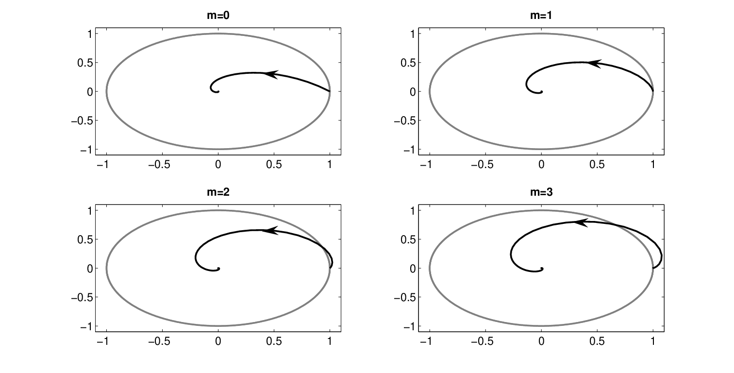
First, we derive the uniform bound (6.19). Using formula (6.22), we calculate
| (6.24) |
and thus , for all . Recalling that , we conclude that all of the eigenvalues lie in the unit disk (equivalently, the th algorithm is stable) for all values of greater than , irrespective of the values of . This is demonstrated in Figure 3.

Next, we derive formulae which describe exactly the stability regions. For , Eq. (6.19) yields . Thus, for all positive values of and for all . As a result, the fixed point is unconditionally stable for positive, values of , see also Figure 3.
For , Eq. (6.22) becomes
Writing for the complex conjugate of , then, we calculate
| (6.25) |
Using this formula, we recast the stability condition (6.23) into the form
In particular, the boundary of the stability region can be obtained by equating the expression in the left member of this inequality to one and solving for , to obtain
Here, and the branch of is chosen so that . We have plotted the stability region in Figure 3. We also note here that the boundary of the stability region close to and to has fine structure, see Figure 4.

6.3 Stability of the fixed point for
In this section, we determine the stability of the fixed point for . We define the function
| (6.29) |
Our results are summarized in the following theorem.
Theorem 6.2
Fix . For each , the functional iteration scheme defined by is stable if and only if, for each , the pair lies in the stability region the boundary of which is given by the implicit equation
where
.
Here,
the branch of
is chosen so that
.
In particular:
(i)
Assume that
,
for all
.
If
,
then
the functional iteration
is unconditionally stable.
If
,
then
the functional iteration
is stable
if and only if
| (6.41) |
(ii) Assume that at least one of is nonzero. If , then a sufficient and uniform (in ) condition for stability is
| (6.42) |
If , the functional iteration is unstable for any and for all
| (6.43) |
As in Section 6.2, we determine when the stability condition (6.20) holds. The analogue of Eqs. (6.21) and (6.22) in this case is, to leading order and for ,
| (6.44) |
The stability condition (6.20) becomes, then,
| (6.45) |
Here also, we distinguish two cases.
Case 1: All of the eigenvalues of are real.
Then, for all , and hence Eq. (6.45) becomes
Plainly, the condition is satisfied for all positive and . Next, solving this equation for , we obtain an equation for the level curve ,
For and for all and positive values of , we obtain (and thus the eigenvalue is stable), see Fig. 5. Therefore, , and the fixed point is unconditionally stable.
For , we obtain the condition , and Eq. (6.41) follows directly. Finally, we note that, for a fixed value of and as , the spectrum clusters around . Thus, the choice is optimal in the sense that large values of bring the spectrum closer to zero.

Case 2: Some of the eigenvalues of have nonzero imaginary parts.
In this case, some of the eigenvalues may become unstable for certain combinations of and , as our analysis in Section 6.2 also showed.
First, we consider the case and derive the uniform bound (6.42). Using formula (6.44) and working as in Eq. (6.24), we estimate
Hence
Combining these inequalities with the stability condition , we obtain the sufficient condition , where is the uniform bound (6.29) (see also Fig. 6). Recalling that , we conclude that, if condition (6.42) is satisfied, then , and hence the th algorithm is stable.
Next, we consider the case and derive the uniform bound (6.43). Equation (6.44) yields
Thus, , for and , and therefore
Hence, is unstable.


Remark.
7 Conclusions and Discussion
In this article, we characterized the accuracy and convergence properties of the class of iterative algorithms introduced in [4] for explicit fast-slow systems (1.2). The -th member of the class corresponds to a functional iteration scheme to solve the st derivative condition (1.10). We showed that this condition has an isolated solution, which corresponds to a fixed point of this -th member and which is accurate up to and including terms of , see Theorem 2.1. Also, we derived explicit formulae for the domain of convergence of the functional iteration, both in the case where analytical formulae for the st derivative are used (see Theorem 3.1) and in the case where the st derivatives are estimated through a forward difference scheme (see Theorem 6.1). These convergence results are illustrated in Figures 1, 3, and 4. Further, we demonstrated how the Recursive Projection Method may be used to stabilize the functional iteration in all cases when it is unstable or to accelerate its convergence in those cases where the convergence is slow.
An extension of the analysis presented here to more general multiscale systems (1.1) will be presented in a subsequent article. The analysis of the accuracy of the st derivative condition presented in Section 2 carries through, essentially (modulo a number of technicalities), in the more general case as well. The analysis of the stability of the functional iteration, on the other hand, is far more involved. The reason for that is that, although the hyperplane and the space tangent to the fast fibration over the slow manifold coincide to leading order for explicit fast–slow systems (1.2), this is not the case for the more general systems (1.1). The absence of this feature makes the stability question for the functional iteration far more difficult to answer in the general case.
In addition, we are in the process of generalizing the results of this article to other maps that may be used in the context of the functional iteration scheme developed in [4]. In particular, it is of interest to use maps which are implicitly defined (as opposed to the explicitly defined ones presented in [4] and in this article). Preliminary analytical results for and indicate that one may construct functional iteration schemes based on implicit maps which not only retain the accuracy of the functional iteration scheme presented in this article but which are also unconditionally stable. Moreover, we think that this analysis may be extended to higher values of , and we note that it is also possible to carry out the functional iteration with implicitly defined maps even when one only has a legacy code as a timestepper.
Appendix A The one-higher-order proposition
In this appendix, we state and prove a technical proposition – called the one-higher-order proposition – about the asymptotic accuracy of approximations of given an approximation of the normal space to . This result is instrumental in the proof of the technical lemmas contained in the next appendix.
We begin by recalling the useful formulation, Eq. (1.15), of the invariance equation that defines the function , whose graph is the invariant, slow manifold . This formulation revealed that the matrix forms a basis for , the space normal to the slow manifold at the point .
The function admits an asymptotic expansion in ,
| (A.1) |
where the coefficients , , are determined by expanding asymptotically the left member of Eq. (1.14) and setting the coefficient of equal to zero to obtain
where the sum is understood to be empty for . The first few equations are
| (A.2) | |||
| (A.3) |
Here, Eq. (A.2) is satisfied identically, Eq. (A.3) yields the coefficient , and so on.
The one-higher-order proposition, which we now state and prove, establishes a connection between the order in to which a set of row vectors approximates and the order to which the solution to the condition approximates .
Proposition A.1
Let be an matrix with the property that its rows span up to and including terms of , for some . That is, is of the form
| (A.4) |
where is a non-singular matrix and , for , in general. Then, the condition
| (A.5) |
can be solved for to yield a function , the asymptotic expansion of which agrees with that of up to and including terms of ,
| (A.6) |
This proposition is called the one-higher-order proposition, because it states that the order to which approximates the full slow manifold is of one higher than that to which approximates the normal space.
Proof of Proposition A.1.
We recall that , by Eq. (A.1), and that is determined from the terms of the invariance equation (1.15). Similarly, is determined from the terms of Eq. (A.5). Thus, to establish Eq. (A.6), it suffices to compare the terms of these two equations from up through and including and to show that they are equal.
First, for each the invariance equation (1.15) at is
| (A.7) |
Second, to derive the terms for the condition , we substitute the hypothesis (A.4) in Eq. (A.5) and left-multiply by to obtain
| (A.8) |
Thus, for each , this condition at is
Plainly, this equation is identical to Eq. (A.7). Thus, , for .
Finally, we look at the terms of the two equations. Eq. (A.7) with is
| (A.9) |
Also, Eq. (A.8) at is
| (A.10) |
We note that , in general. However, , since the terms appearing in Eqs. (A.9)–(A.10) are evaluated at . Thus, Eqs. (A.9) and (A.10) also agree, and hence . This completes the proof of the proposition.
Appendix B Proofs of Lemmata 2.1 and 2.2
In this appendix, we prove lemmata 2.1 and 2.2 characterizing the asymptotic accuracy of the approximation to obtained from the st derivative condition (2.10).
Proof of Lemma 2.1.
We write for and for . The strategy is as follows: We will show that the rows of span up to and including terms of . Then, we will apply Proposition A.1 to establish Eq. (2.12).
The manifold is the graph of the function , and thus it coincides exactly with the zero level set of the function . As a result, the rows of the gradient matrix form a basis for . Second, the function is defined through the st derivative condition . Therefore, also coincides with (a connected component of) the zero level set of the function . Thus, the rows of the gradient matrix also form a basis for . It follows from the existence of these two bases that there exists a non-singular matrix such that
| (B.1) |
Next, the induction hypothesis implies that the asymptotic expansions of and agree up to and including terms of ,
| (B.2) |
Since the vector field is assumed to be sufficiently smooth, we may differentiate both sides of this equation with respect to to obtain
| (B.3) |
Combining Eqs. (B.1) and (B.3), then, we find
This equation shows that the rows of span up to and including terms of . Hence, application of the one-higher-order proposition, Proposition A.1, completes the proof of this lemma.
Before we proceed with the proof of Lemma 2.2, we prove the following result which will be needed therein.
Lemma B.1
For , for , and for a general point , the function is written as
where the notation “” stands for . The Jacobian is written as
| (B.4) |
Proof. For this proof, we write instead of for the sake of brevity. The proof is by induction on . For , we recall Eq. (2.4),
and hence, expanding in powers of , we find
This is the desired formula for . Differentiating both members of this formula with respect to , we obtain
This is the desired formula for .
Next, we carry out the induction step for general , namely we assume that
| (B.5) | |||||
| (B.6) |
and show that
| (B.7) | |||||
| (B.8) |
By Eq. (2.9),
Then, we substitute the induction hypothesis (B.5) into this expression. Application of the differential operator on the remainder does not alter its asymptotic magnitude. Moreover, the term is and, hence, can be absorbed also in the remainder. Therefore, we are left with the term . Substituting into this expression from the induction hypothesis (B.6), we arrive at the desired formula (B.7).
Finally, we prove the leading order formula (B.8). First, we differentiate both members of the leading order formula (B.7) with respect to and use the product rule derivative to evaluate the right member. The second term from the product rule is precisely the leading order term in Eq. (B.4). The other term from the product rule,
may be absorbed in the remainder since it is linear in . Thus, we have obtained the desired formula (B.8) and completed the proof of the lemma.
Proof of Lemma 2.2.
We first use [2, Theorem 3] to establish that condition (2.10) has a solution which is close to . According to that theorem, it suffices to show that
By the definition of ,
Thus, we may write
| (B.9) | |||||
Next, we have the following estimates of the asymptotic magnitudes of the two terms in the right member of Eq. (B.9):
by Lemma 2.1, and also
by the induction hypothesis. Thus,
and hence Taylor’s Theorem with remainder yields
| (B.10) |
since and its derivatives are . This is the desired estimate of the first term in the right member of Eq. (B.9).
It remains to estimate the second term, in the right member of Eq. (B.9). We recall that , where and are in general. Hence, the first component of is plainly . The second component is as well, since Lemma 2.1 implies that and hence that , also. Therefore,
| (B.11) |
Combining the estimates (B.10) and (B.11), we see that the right member of Eq. (B.9) is , which is the desired result.
Finally, the solution of the condition yields an dimensional manifold , as may be shown using the Implicit Function Theorem and [14, Theorem 1.13]. It suffices to show that
Lemma B.1 yields a leading order formula for ,
Here, is a general point and . Next, we showed above that . Recalling, then, Eq. (2.5), we obtain
where . Thus,
by normal hyperbolicity and the proof is complete.
References
- [1] G. Browning, H.-O. Kreiss, Problems with different time scales for nonlinear partial differential equations, SIAM J. Appl. Math. 42(4) (1982) 704–718
- [2] J. Carr, Applications of Centre Manifold Theory, Applied Mathematical Sciences, 35, Springer–Verlag, New York, 1981
- [3] J. Curry, S. E. Haupt, M. E. Limber, Low-order modeling, initializations, and the slow manifold, Tellus 47A (1995) 145–161
- [4] C. W. Gear, T. J. Kaper, I. G. Kevrekidis, and A. Zagaris, Projecting to a Slow Manifold: Singularly Perturbed Systems and Legacy Codes, SIAM J. Appl. Dyn. Syst. 4 (2005) 711–732
- [5] C. W. Gear and I. G. Kevrekidis, Constraint-defined manifolds: a legacy-code approach to low-dimensional computation, J. Sci. Comp., 25(1) (2005), 17–28
- [6] S. S. Girimaji, Reduction of large dynamical systems by minimization of evolution rate, Phys. Rev. Lett., 82 (1999), 2282–2285
- [7] C. K. R. T. Jones, Geometric singular perturbation theory, in: Dynamical Systems, Montecatini Terme, L. Arnold, Lecture Notes in Mathematics, 1609, Springer-Verlag, Berlin, 1994, pp. 44–118
- [8] H. G. Kaper and T. J. Kaper, Asymptotic analysis of two reduction methods for systems of chemical reactions, Physica D 165 (2002), 66–93
- [9] C. T. Kelley, Iterative Methods for Linear and Nonlinear Equations, Frontiers In Applied Mathematics, 16, SIAM Publications, Philadelphia, 1995
- [10] I. G. Kevrekidis, C. W. Gear, J. M. Hyman, P. G. Kevrekidis, O. Runborg, and C. Theodoropoulos, Equation-free, coarse-grained multiscale computation: enabling microscopic simulators to perform system-level analysis, Commun. Math. Sci. 1 (2003) 715–762
- [11] H.-O. Kreiss, Problems with different time scales for ordinary differential equations, SIAM J. Numer. Anal. 16(6) (1979) 980–998
- [12] H.-O. Kreiss, Problems with Different Time Scales, in Multiple Time Scales, J. H. Brackbill and B. I. Cohen, eds., Academic Press, 1985, pp. 29-57
- [13] E. N. Lorenz, Attractor sets and quasi-geostrophic equilibrium, J. Atmos. Sci. 37 (1980) 1685–1699
- [14] P. J. Olver, Applications of Lie Groups to Differential Equations, Graduate Texts in Mathematics, 107, Springer–Verlag, New York, 1986
- [15] G. M. Shroff and H. B. Keller, Stabilization of unstable procedures: A recursive projection method, SIAM J. Numer. Anal. 30 (1993) 1099–1120
- [16] P. van Leemput, W. Vanroose, and D. Roose, Initialization of a Lattice Boltzmann Model with Constrained Runs, Report TW444, Catholic University of Leuven, 2005
- [17] P. van Leemput, C. Vandekerckhove, W. Vanroose, and D. Roose, Accuracy of hybrid Lattice Boltzmann/Finite Difference schemes for reaction-diffusion systems, Multiscale Model. Sim., to appear
- [18] A. Zagaris, H. G. Kaper, and T. J. Kaper, Analysis of the Computational Singular Perturbation reduction method for chemical kinetics, J. Nonlin. Sci. 14 (2004) 59–91
- [19] A. Zagaris, H. G. Kaper, and T. J. Kaper, Fast and slow dynamics for the Computational Singular Perturbation method, Multiscale Model. Sim. 2 (4) (2004) 613–638