Constraints on Neutralino masses and mixings
from Cosmology and Collider Physics
Dissertation
zur
Erlangung des Doktorgrades (Dr. rer. nat.)
der
Mathematisch-Naturwissenschaftlichen Fakultät
der
Rheinischen Friedrich-Wilhelms-Universität
zu Bonn
vorgelegt von
Ulrich Langenfeld
geb. in
Neuwied
Bonn 2007
Angefertigt mit Genehmigung der Mathematisch-Naturwissenschaftlichen Fakultät der Universität Bonn.
Referent: Prof. Herbert Dreiner Korreferent: Prof. Manuel Drees Tag der Promotion:
Ich versichere, daß ich diese Arbeit selbständig verfaßt und keine anderen als die angegebenen Quellen und Hilfsmittel benutzt sowie die Zitate kenntlich gemacht habe.
Referent: Prof. Herbert Dreiner Korreferent: Prof. Manuel Drees
To my parents
Acknowledgements
First I would like to express my gratitude to my supervisor Herbi Dreiner for his help and support with this work.
Furthermore I thank Manuel Drees for enlightening discussions on dark matter and acting as second referee for this thesis.
I also thank I. Brock, K. Desch, G. Moortgat-Pick, M. Schumacher, X. Tata and G. Weiglein for helpful discussions.
I am also grateful to my collaborator as well as room mate Olaf Kittel for the effective and also fun research, he provided the Fortran code for the neutralino pair production to me and read parts of the manuscript.
I have always enjoyed the friendly atmosphere in our group and the enspiring discussions with Olaf Kittel, Federico von der Pahlen, Markus Bernhardt, Jong Soo Kim, Sebastian Grab, Anja Marold and Chung-Lin Shan.
In addition I would like to thank our always helpful secretaries of the Bonn theory group, namely D. Fassbender, P. Zündorf, and S. Heidbrink and our computer and allround specialist A. Wisskirchen.
My parents supported me during the time this work was being done. I am very grateful to them.
Chapter 0 Abstract
Bounds on cross section measurements of chargino pair production at LEP yield a bound on the chargino mass. If the GUT relation is assumed, then the lightest neutralino must be heavier than . If is considered as a free parameter independent of there is no bound on the mass of the lightest neutralino. In this thesis, I examine consequences of light, even massless neutralinos in cosmology and particle physics.
In Chapter 2, I discuss mass bounds on the lightest neutralino from relic density measurements. The relic density can be calculated by solving the Boltzmann equation. If the relic density is considered as a function of the particle mass then there are two mass regions where the relic density takes on realistic values. In the first region the neutralino is relativistic and its mass must be lower than , in the second region the neutralino is nonrelativistic and must be heavier than . I compare the Cowsik-McClelland bound, the approximate solution of a relativistic particle for the Boltzmann equation, and the Lee-Weinberg bound, the non-relativistic approximation, with the full solution and I find that the approximation and the full solution agree quite well.
In Chapter 3, I derive bounds on the selectron mass from the observed limits on the cross section of the reaction at LEP, if the lightest neutralino is massless. If , the selectron must be heavier than .
In Chapter 4, I study radiative neutralino production at the linear collider with longitudinally polarised beams. I consider the Standard Model background from radiative neutrino production , and the supersymmetric radiative production of sneutrinos , which can be a background for invisible sneutrino decays. I give the complete tree-level formulas for the amplitudes and matrix elements squared. In the Minimal Supersymmetric Standard Model, I study the dependence of the cross sections on the beam polarisations, on the parameters of the neutralino sector, and on the selectron masses. I show that for bino-like neutralinos longitudinal polarised beams enhance the signal and simultaneously reduce the background, such that search sensitivity is significantly enhanced. I point out that there are parameter regions where radiative neutralino production is the only channel to study SUSY particles at the ILC, since heavier neutralinos, charginos and sleptons are too heavy to be pair-produced in the first stage of the linear collider with .
In Section 7, I focus on three different mSUGRA scenarios in turn at the Higgs strahlung threshold, the top pair production threshold, and at . In these scenarios at the corresponding , radiative neutralino production is the only supersymmetric production mechanism which is kinematically allowed. The heavier neutralinos, and charginos as well as the sleptons, squarks and gluinos are too heavy to be pair produced. I calculate the signal cross section and also the Standard Model background from radiative neutrino production. For my scenarios, I obtain significances larger than and signal to background ratios between and , if I have electron beam polarization and positron beam polarization . If I have electron beam polarization of , then the signal is observable with but both the significance and the signal to background ratio are significantly improved for .
In Chapter 5, I present a method to determine neutralino couplings to right and left handed selectrons and bosons from cross section measurements of radiative neutralino production and neutralino pair production , at the ILC. The error on the couplings is of order . From the neutralino couplings the neutralino diagonalisation matrix can be calculated. If all neutralino masses are known, , , and can be calculated with an error of the order . If also the cross sections of the reactions can be measured the error of , , and reduces to .
Chapter 1 The Gaugino sector in the MSSM
The Standard Model (SM) has been tested to high precision. But many problems remain unsolved. The SM does not include gravity. The electro-weak couplings and the strong coupling do not unify in a point at the GUT scale . The SM model cannot explain why there is so much more matter than antimatter in the universe and it does not provide a dark matter candidate.
One solution to these problems is supersymmetry [1, 2, 3, 4, 5]. In supersymmetric theories, each fermion is mapped onto a boson and vice versa. The spin of the fermion and its partner boson differ by half a unit, the other quantum numbers are unchanged.
The superpartners of leptons, quarks, gauge bosons, and Higgs bosons are called sleptons, squarks, gauginos, and higgsinos, respectively. The two neutral gauginos , and the two neutral higgsinos , have the same quantum numbers and mix. The physical mass eigenstates are obtained by diagonalisation of the mass matrix. These neutral particles are called neutralinos. They are Majorana fermions. The two charged gauginos and two charged higgsinos mix to charginos.
At low energies no SUSY particles have been observed, so SUSY must be broken. The most common way is introducing explicitly soft SUSY breaking terms.
The part of the Lagrangian which describes the neutralino mixing is given by [4]
| (1) | |||||
| with | |||||
| (2) | |||||
| (3) |
and are the and the gaugino mass parameters, respectively. They break SUSY explicitly. is the higgsino mass parameter and is the ratio of the two vacuum expectation values of the Higgs fields, the boson mass, and the weak mixing angle.
, , and are real parameters, if is conserved, in general they are complex:
| (4) |
The matrix is symmetric, even for complex. The reason for this fact is that in Eq. 1 there appear no hermitian conjugated fields. The matrix can be diagonalised by an unitary matrix using Takagi’s factorization theorem [6]
| (5) |
The diagonal elements are non-negative and are the square roots of the eigenvalues of . The transformation Eq. (5) is not a similarity transformation, if is complex.
If is a real matrix it can also be diagonalised by an orthogonal matrix. From the lower right submatrix one can see that at least one eigenvalue is negative. This sign is interpreted as the eigenvalue of the neutralino. The masses of the neutralinos are , . The sign can be absorbed in a phase of the corresponding eigenvector, leading back to Eq. (5).
The eigenvalues of and the diagonalisation Matrix can be obtained algebraically, see Ref. [7] or numerically. The algebraic method is problematic because it is numerically unstable. Gunion and Haber present in [8] approximate solutions to the eigenvalues of and the diagonalisation matrix , if .
Without loss of generality can be chosen positive. Proof: Let . The phase of can be removed by the transformations:
| (6) |
The parameters and transform as
| (7) | |||||
| (8) |
It is not necessary to transform the higgsino fields. Alternatively, the vacuum expectation values can be transformed as leaving invariant.
If then the signs of and are interchanged. This transformation reverses also the sign of the eigenvalues of .
In GUT theories, and are related by
| (9) |
It follows that and can be chosen positive.
can have zero eigenvalues. From it follows in the conserving case, see Ref. [9],
| (10) | |||||
The solution is excluded due to experimental constraints from the -widths measured at LEP [10].
In the violating case, substitute , with , . This yields two equations, which must be separately fulfilled:
| (11) | |||||
| (12) |
or
| (13) |
or
| (14) |
It follows immediately that and must hold. Also in the violating case one can always find parameters , and to get .
The chargino mixing is described by the following matrix:
| (15) | |||||
| (16) | |||||
| (17) |
is not symmetric, so it must be diagonalised by a biunitary transformation:
| (18) |
with , unitary matrices. The matrices and are obtained by solving
| (19) |
The eigenvalues can be obtained analytically, see Ref. [1, 2]. In practical use it is easier to diagonalize the matrix numerically but using the analytical formulae.
The lower experimental bound on the lightest chargino mass is [11]. This bound leads to lower bounds on and : . If Eq. (9) is assumed, then depends on and from this fact follows a lower bound on the mass of the lightest neutralino: [12]. But up to now there is no evidence that Eq. (9) holds. So I consider as a free parameter. In the following I study implications of massless and light neutralinos. In Chapter 2, I discuss bounds on the neutralino mass from dark matter density measurements. In Chapter 3, I derive bounds on the selectron mass from the observed cross section limits from production at LEP, if is massless. In Chapter 4, I calculate the cross section for radiative neutralino production and its neutrino and sneutrino background at a future linear collider. I discuss the influence of beam polarisation on radiative neutralino production and consequences of SUSY searches at a future linear collider. Finally, in Chapter 5, I present a method how to determine neutralino couplings to the right and left handed selectron and the boson.
Chapter 2 Cosmological bounds on neutralino masses
1 The Cowsik-McClelland-bound
I derive bounds on the mass of the lightest neutralino through cosmological considerations. Neutralinos are neutral and interact only weakly. If they are (pseudo-)stabile, they are dark - matter (DM) candidates. The dark matter density has been measured by the WMAP collaboration [13]. This constrains the mass(es) of the particle(s) which constitute the dark matter.
In Ref. [14], Kolb and Turner describe the thermal evolution of the Universe and its impact on particle physics. I give a short summary in order to clarify the subsequent section.
1.1 The Expansion of the Universe
The expansion of the Universe is described by the Einstein field equations with the Robertson-Walker (RW) metric. In the RW metric, the Universe is assumed to be homogeneous and isotropic.
| (20) | |||||
| (21) | |||||
| (22) |
Here is the cosmic scale factor, and denote the pressure and the density, respectively, and is Newton’s constant. Eq. (20) is called the Friedmann equation, Eq. (22) is the 1st law of thermodynamics. The parameter can be chosen as or to describe spaces with constant positive or negative curvature, or flat geometry, respectively. Eq. (20) and Eq. (21) can be subtracted to yield an equation for the acceleration of the scale factor
| (23) |
The Hubble parameter determines the expansion of the Universe. It is defined as . The present day value is called the Hubble constant. With this definition the critical density —the density, where the geometry of the Universe is flat— follows as . To solve Eqs. (20) - (22) we need an additional ingredient: an equation of state, that describes the connection between density and pressure of the matter content of the Universe (i.e. radiation, baryonic matter or dark energy). At the beginning, the Universe was dominated by radiation, after recombination the photons decoupled and the Universe was matter dominated. Today the dark energy contributes most of the density of the Universe. The equations of state are
| (24) | |||||
| (25) | |||||
| (26) |
The Eqs (24)-(26) can be summarized to
| (27) |
for radiation, matter, and dark energy, respectively. The dark energy is connected to the cosmological constant in the Einstein field equation.
1.2 Basic Thermodynamics
The particle density, the energy density and the pressure of a particle species in the Universe are given by
| (28) | |||||
| (29) | |||||
| (30) |
where the phase space distribution (or occupancy) is given by
| (31) |
The sign holds for fermions, the for bosons, and is the chemical potential of the particles species. The energy of a relativistic particle is given by . The entropy follows from
| (32) |
1.3 Particles in the Universe
I consider the behaviour of a class of particles , (f. e. sparticles in the MSSM) in the thermal bath of the early Universe. Griest and Seckel discuss in [15] the mechanisms that are important in order to determine the number density of these new particles. They assume that the have a multiplicatively conserved quantum number which distinguish them from Standard Model (SM) particles. In the MSSM, parity [16] is such a quantum number. The subsequent reactions appear:
| (33a) | ||||
| (33b) | ||||
| (33c) | ||||
where , denote SM particles. Examples in the MSSM for these three reaction types are:
| (34a) | ||||
| (34b) | ||||
| (34c) | ||||
respectively. One of these particles is stabile due to the conserved quantum number. In the MSSM with conserved R-parity, it is the . Griest and Seckel classify the reaction types, see Eq. (33), further. If the lightest is nearly mass degenerate to the next to lightest particle , then the number density of is also determined by annihilations of which decays later into . This is called coannihilation. The masses of annihilation products can be heavier than the masses of the ingoing particles, if the energy of the ingoing particles is large enough. Griest and Seckel call this ”forbidden” channels. If annihilation occurs at a pole in the cross section it is called annihilation near a pole or resonant annihilation.
For the further discussion, I exclude coannihilation and resonant annihilation for simplicity.
The time evolution of a particle with total cross section is described by the Boltzmann equation:
| (35) |
with the the particle velocity . The second term accounts for the dilution of the species due to the expansion of the Universe, the third term for the decrease by annihilation into other particles or coannihilation with other particles. If we define
| (36a) | ||||
| (36b) | ||||
| (36c) | ||||
| (36d) | ||||
| (36e) | ||||
| (36f) | ||||
then Eq. (35) can be cast into
| (37) |
or
| (38) |
is the number of massless degrees of freedom at , where the particle temperature accounts for the possibility that it is different from the photon temperature . The thermal averaged cross section is defined as
| (39) |
If , then does not change with time, so it is constant as expected, c. f. Eq. (39). If , then the relative change of is small and the annihilation processes stop, which means that the number of that particle species remains constant within a comoving volume.
1.4 Application to Massless Neutralinos
In the MSSM with -parity conservation, the lightest neutralino is stabile and can be the lightest supersymmetric particle. Therefore it is a dark matter candidate. I discuss the case when the neutralino is (nearly) massless, . The width allows a higgsino contribution of about , see Choudhury et al. [10]. , the bino-mass, is normally chosen smaller than and , and so the lightest neutralino is almost bino. For simplicity, I assume that it is purely bino. The neutralino freezes out at , and at freeze out it is still relativistic. From that it follows .
| (40) |
where and are given by Eq. (28) and (36a), is the present entropy density, and denotes the Riemannian Zeta function. It is assumed that the entropy per comoving volume is conserved. counts the degrees of freedom of the neutralino field multiplied with to correct for the fermionic nature of the field, counts the number of relativistic fields at freeze out, whereby fermionic fields are corrected with :
| (41) | |||||
The neutralino density is obtained by
| (45) | |||||
| (46) |
In Eq. (46) I relate the relic density to the photon temperature by using and to the critical density. The constraint on the density is chosen such that the lightest neutralino does not disturb structure formation, so they cannot form the dominant component of the dark matter.
Light neutralinos decouple at . This temperature is somewhat higher than the temperature, when the neutrinos decouple. This is due to the selectron mass which can be larger than the mass, leading to smaller cross sections. But the temperature is below the muon mass so that it is not necessary to know the exact value. Nevertheless we have 2 bosonic and 12 fermionic relativistic degrees of freedom (one Dirac electron, three left handed neutrino species, one photon, one light Majorana neutralino) leading to and . If I demand (value of taken from WMAP [13])
| (47) |
then it follows
| (48) |
This idea is due to Gershtein and Zel’dovich [17] and Cowsik and McClelland [18] to derive neutrino mass bounds.
2 The Lee - Weinberg bound
In this section, I discuss mass bounds for heavy nonrelativistic neutralinos with . I use the same method as proposed by various authors independently in [19, 20, 21, 22] to constrain heavy neutrinos. This bound is now referred as Lee - Weinberg bound.
This case is not as easy, the thermal averaged cross section and the freeze out temperature have to be calculated to yield an approximate solution of the Boltzmann equation.
For simplicity, I consider only the neutralino annihilation into leptons
| (49) |
The is considered as massless 11 1 For a lower mass bound of about , this is a good approximation, but not for neutralino masses of the order [23]., all sleptons have common mass (not to be confused with the common scalar mass parameter ), so the cross sections are related by
| (50) |
The thermal averaged cross section Eq. (39) can be calculated using the techniques described in [24]. This leads to a parametrisation of the form . In the case of a bino the thermal averaged cross section reads
| (51) |
with defined in Eq. (36c). The Boltzmann Equation can be cast into the form
| (52) |
Let the difference denote the deviation of the particle density of the bino from equilibrium density . Shortly after the Big Bang, the deviation and its derivative are small. Therefore, a good approximation is setting , and one gets:
| (53) |
Later after decoupling, the neutralinos are no longer in thermal equilibrium, and the terms involving can be neglected. So one gets the following differential equation:
| (54) |
To solve Eq. (54), we have to integrate from to . Recall, that we transformed the time dependence of the Boltzmann equation into an -dependence by the transformations Eq. (36c-36f). The solutions for Eqs (53) and (54) are
Eq. (2) requires the knowledge of the freeze out temperature or, equivalently, . The decoupling temperature is the temperature, when the deviation has grown to order . One sets , , and solves Eq. (53) for , yielding
| (58) | |||||
| (59) | |||||
| (60) | |||||
| (61) |
The choice [14] has been implemented and yields the best fit to the relic density. There is a remarkable feature of Eq. (61): The lower the cross section the larger the relic density. This can be understood: The particle density distribution is a Boltzmann distribution. If the cross section is large the particles stay longer in thermal equilibrium, and the particle density decreases stronger with falling temperature.
In Fig. 1(a), I show contours of constant relic density in the - -plane. The lower right hand triangle of the figure is excluded since the sleptons are lighter than the neutralino. In Fig. 1(b), I show the contours limiting the area ([25]), denotes the absolute error on . The horizontal line indicates the approximate lower bound on the slepton masses of about . If we demand that the neutralinos constitute the whole dark matter and that the sleptons are heavier than , we find a lower mass bound of the neutralinos of about . The masses of the slepton cannot exceed . If the next to lightest supersymmetric particle is heavier than , the neutralino mass bounds are
| (62) |


The result shows the advantage of estimating the neutralino mass from the dark matter density form an approximation rather than doing the full calculation: There are only two (or three) parameters (, , or ), which can be plotted in a two dimensional figure.
3 Numerical solution of the full Boltzmann equation
In the previous section, I derived from an approximate solution of the Boltzmann equation an upper and lower bound on the neutralino mass and – with caution – for the slepton mass. Now I compare these results with the exact solution. For this purpose I use the program micrOMEGAs [27].
The estimation does not take into account coannihilation and resonant annihilation. Near the threshold where the neutralino is almost mass degenerate with the sleptons there is coannihilation. And even for a small Higgsino component, there is large resonant annihilation if the neutralino mass is half of the -mass or half of the -mass.


In Fig. 2, I show contour lines of the relic density for the following scenario: , , = , , , , . The masses of the sleptons and of the lightest neutralino are varied. The masses of the particles other than sleptons are kept constant, so one can directly see the influence of the particle masses on the relic density. Electron and muon are considered as massless, and the choice of leads to equal slepton masses. The corner at the bottom right is excluded since the neutralino is heavier than the sleptons. Contrary to the Lee-Weinberg-approximation, the exact solution includes coannihilation near the line . Fig. 2(a) shows also the influence of a (small) Higgsino component, leading to resonant annihilation due to and bosons. The resonance increases the cross section dramatically. This allows for larger slepton masses. The two resonances appear in Fig. 2(a) as two valleys in the - plane at and . From this I conclude that in realistic models no bound can be set on the slepton mass by relic density calculations. As lower bound on the neutralino mass I get
| (63) |
This agrees with the lower bound from the approximation. The upper bound is given by the mass of the next to lightest supersymmetric particle (nlsp). For comparison Fig. 2(b) shows the approximate and the exact solution overlayed in one plot. Apart from the valleys both plots agree quite well.
If non-relativistic neutralinos constitute the whole dark matter, they cannot be completely annihilated due to resonant annihilation. This means that the mass of the neutralino is sufficiently far away from the relations or .
Fig. 2(c) shows for one parameter set (, , , as common slepton mass, as common squark mass, , and ) the relic density as a function of the neutralino mass. has been increased from to to vary the neutralino mass. The two spikes at the end of the curve stem from resonant annihilation due to the and the resonance. The nlsp has a mass of about . The qualitative shape of the curve is similar to the curve published in [14].
The horizontal red dashed lines are lines with with , . The black curve crosses the allowed ribbon twice: at very light neutralinos with mass and at massive neutralinos with mass . In the first case the particles which constitute the dark matter cannot only be neutralinos because too many relativistic particles disturb structure formation in the early Universe. To avoid this constraint the neutralinos are only allowed to contribute as much as the neutrinos. This lowers the neutralino mass bound a little bit. The bound for relativistic neutralinos agrees very well with the predictions of the Cowsik-McClelland-bound.
The exact value of the lower mass bound in the nonrelativistic case depends on the parameters of the model (slepton and squark masses, mass difference to the nlsp, resonant annihilation). The upper bound is rather trivial, it is the next to lightest supersymmetric particle. Such searches need a lot of CPU time and have recently been done by Hooper and Plehn [28], Bottino and al. [23] and Belanger et al. [29]. Hooper and Plehn found a lower bound of about for a nonrelativistic neutralino, Bottino et al. found a lower bound of about , and Belanger et al. found a lower neutralino mass bound of about in models with a light pseudoscalar Higgs with mass .
Chapter 3 --production at LEP
In this chapter, I derive mass bounds on the selectron mass from upper limits on the cross section measured by the OPAL collaboration at LEP [30], if the lightest neutralino is assumed as massless. These bounds on the cross section translate into bounds on the selectron mass. I assume equal right and left handed selectron masses.
The Delphi [12] and the Opal collaboration [30] have searched for SUSY particles. For neutralino pair production
| (64) |
they present upper bounds on the cross sections in the - plane. Their analysis assumes that the hadronic channels have a . The selectron mass is assumed to be . So the two body decays into selectrons is not possible. The production of in collision occurs either by channel exchange of a boson or via and channel selectron exchange. For massless neutralinos, the is nearly pure bino (), so it couples preferably to , the is mostly wino and couples stronger to . Due to the large selectron mass the and channel contributions to the cross section are suppressed, so the dominant contribution comes from the channel. The interference between and selectron exchange is positive. If I denote the total cross section as then the contribution becomes larger, if the selectron is lighter, . This ensures that the experimental limits on the cross section are also applicable for selectrons with mass . Therefore, the reported bounds on the cross section are absolute upper bounds.
In Fig. 3(a), I show contour lines for the cross section with and in the - plane for chosen such that is massless. The cross section reaches values up to . There is a large parameter region where the cross section exceeds . From Fig. 3(d), taken from [30], one reads off that for a massless the maximally allowed cross section is about at (At , there are dark grey spots, indicating that the allowed cross section is . They are most likely due to fluctuations in the data, I ignore them for simplicity). Within the contour line and the contour line the cross section is larger than and so this part of the parameter space is ruled out (note that and are nearly mass degenerate).
In Fig. 3(b), I show contour lines of the minimal selectron mass so that the limits from Fig. 3(d), , are fulfilled. The upper black line indicates the kinematical limit. Below the lower black line, the is lighter than , which is experimentally excluded [11]. Along the blue contour the and the selectrons have equal masses at about . Above the blue line the selectrons are lighter than and the two body decay is allowed. For no part of the parameter space can be excluded. In Fig. 3(c), I show contour lines for the mass of in the - plane.
For the OPAL bound is only fulfilled if the selectrons are heavier than . For , as in the SPS1a scenario, the right handed selectron must be heavier than .
Conclusion: The experimental limits on the cross section by OPAL set severe bounds on the selectron mass if and .


Chapter 4 Radiative Neutralino Production
4 Introduction
Supersymmetry (SUSY) is an attractive concept for theories beyond the Standard Model (SM) of particle physics. SUSY models like the Minimal Supersymmetric Standard Model (MSSM) [1, 31, 5] predict SUSY partners of the SM particles with masses of the order of a few hundred GeV. Their discovery is one of the main goals of present and future colliders in the TeV range. In particular, the international linear collider (ILC) will be an excellent tool to determine the parameters of the SUSY model with high precision [32, 33, 34, 35, 36]. Such a machine provides high luminosity , a center-of-mass energy of in the first stage, and a polarised electron beam with the option of a polarised positron beam [37].
The neutralinos are the fermionic SUSY partners of the neutral gauge and CP-even Higgs bosons. Since they are among the lightest particles in many SUSY models, they are expected to be among the first states to be observed. At the ILC, they can be directly produced in pairs
| (65) |
which proceeds via boson and selectron exchange [38, 39]. At tree level, the neutralino sector depends only on the four parameters , , , and , which are the and gaugino masses, the higgsino mass parameter, and the ratio of the vacuum expectation values of the two Higgs fields, respectively. These parameters can be determined by measuring the neutralino production cross sections and decay distributions [35, 40, 41, 42, 43]. In the MSSM with R-parity (or proton hexality, , [26]) conservation, the lightest neutralino is typically the lightest SUSY particle (LSP) and as such is stable and a good dark matter candidate [44, 45]. In collider experiments the LSP escapes detection such that the direct production of the lightest neutralino pair
| (66) |
is invisible. Their pair production can only be observed indirectly via radiative production
| (67) |
where the photon is radiated off the incoming beams or off the exchanged selectrons. Although this higher order process is suppressed by the square of the additional photon-electron coupling, it might be the lightest state of SUSY particles to be observed at colliders. The signal is a single high energetic photon and missing energy, carried by the neutralinos.
As a unique process to search for, the first SUSY signatures at colliders, the radiative production of neutralinos has been intensively studied in the literature [46, 47, 48, 49, 50, 51, 52, 53, 54, 55, 56, 57, 58, 59, 60, 61, 62].22 2 In addition I found two references [63, 64], which are however almost identical in wording and layout to Ref. [58]. Early investigations focus on LEP energies and discuss special neutralino mixing scenarios only, in particular the pure photino case [46, 47, 48, 49, 50, 51, 52, 53]. More recent studies assume general neutralino mixing [54, 55, 56, 57, 58, 59, 60, 61, 62] and some of them underline the importance of longitudinal [54, 55, 56, 57] and even transverse beam polarisations [54, 57]. The transition amplitudes are given in a generic factorised form [55], which allows the inclusion of anomalous couplings. Cross sections are calculated with the program CompHEP [56], or in the helicity formalism [57]. Some of the studies [58, 59, 60, 61, 62] however do not include longitudinal beam polarisations, which might be essential for measuring radiative neutralino production at the ILC. Special scenarios are considered, where besides the sneutrinos also the heavier neutralinos [59, 60, 61], and even charginos [65, 66, 67] decay invisibly or almost invisibly. However, a part of such unconventional signatures are by now ruled out by LEP2 data [59, 66, 68]. For the ILC, such “effective” LSP scenarios have been analysed [60], and strategies for detecting invisible decays of neutralinos and charginos have been proposed [65, 67]. Moreover, the radiative production of neutralinos can serve as a direct test to see, whether neutralinos are dark matter candidates. See for example Ref. [69], which presents a model independent calculation for the cross section of radiatively produced dark matter candidates at high-energy colliders, including polarised beams for the ILC.
The signature “photon plus missing energy” has been studied intensively by the LEP collaborations ALEPH [70], DELPHI [71], L3 [72], and OPAL [68, 73]. In the SM,
| (68) |
is the leading process with this signature. Since the cross section depends on the number of light neutrino generations [74], it has been used to measure consistent with three. In addition, the LEP collaborations have tested physics beyond the SM, like non-standard neutrino interactions, extra dimensions, and SUSY particle productions. However, no deviations from SM predictions have been found, and only bounds on SUSY particle masses have been set, e.g. on the gravitino mass [70, 71, 72, 73]. This process is also important in determining collider bounds on a very light neutralino [75]. For a combined short review, see for example Ref. [76].
Although there are so many theoretical studies on radiative neutralino production in the literature, a thorough analysis of this process is still missing in the light of the ILC with a high center-of-mass energy, high luminosity, and longitudinally polarised beams. As noted above, most of the existing analyses discuss SUSY scenarios with parameters which are ruled out by LEP2 already, or without taking beam polarisations into account. In particular, the question of the role of the positron beam polarisation has to be addressed. If both beams are polarised, the discovery potential of the ILC might be significantly extended, especially if other SUSY states like heavier neutralino, chargino or even slepton pairs are too heavy to be produced at the first stage of the ILC at GeV. Moreover, the SM background photons from radiative neutrino production have to be included in an analysis with beam polarisations. Proper beam polarisations could enhance the signal photons and reduce those from the SM background at the same time, which enhances the statistics considerably. In this respect also the MSSM background photons from radiative sneutrino production
| (69) |
have to be discussed, if sneutrino production is kinematically accessible and if the sneutrino decay is invisible.
Finally, the studies which analyse beam polarisations do not give explicit formulas for the squared matrix elements, but only for the transition amplitudes [54, 55, 57]. Other authors admit sign errors [61] in some interfering amplitudes in precedent works [60], however do not provide the corrected formulas for radiative neutrino and sneutrino production. Additionally, I found inconsistencies and sign errors in the exchange terms in some works [54, 57], which yield wrong results for scenarios with dominating exchange. Thus I will give the complete tree-level amplitudes and the squared matrix elements including longitudinal beam polarisations, such that the formulas can be used for further studies on radiative production of neutralinos, neutrinos and sneutrinos.
In Sec. 5, I discuss my signal process, radiative neutralino pair production, as well as the major SM and MSSM background processes. In Sec. 6, I define cuts on the photon angle and energy, and define a statistical significance for measuring an excess of photons from radiative neutralino production over the backgrounds. I analyse numerically the dependence of cross sections and significances on the electron and positron beam polarisations, on the parameters of the neutralino sector, and on the selectron masses. I summarise and conclude in Sec. 8. In the Appendix, I define neutralino mixing and couplings, and give the tree-level amplitudes as well as the squared matrix elements with longitudinal beam polarisations for radiative production of neutralinos, neutrinos and sneutrinos. In addition, I give details on the parametrisation of the phase space.
5 Radiative Neutralino Production and Backgrounds
5.1 Signal Process
Within the MSSM, radiative neutralino production [46, 47, 48, 49, 50, 51, 52, 53, 54, 55, 56, 57, 58, 59, 60, 61, 62]
| (70) |
proceeds at tree-level via - and -channel exchange of right and left selectrons , as well as boson exchange in the -channel. The photon is radiated off the incoming beams or the exchanged selectrons; see the contributing diagrams in Fig. 4. I give the relevant Feynman rules for general neutralino mixing, the tree-level amplitudes, and the complete analytical formulas for the amplitude squared, including longitudinal electron and positron beam polarisations, in Appendix 6. I also summarise the details of the neutralino mixing matrix there. For the calculation of cross sections and distributions I use cuts, as defined in Eq. (77). An example of the photon energy distribution and the dependence of the cross section is shown in Fig. 5.
1.0 \SetWidth0.7
5.2 Neutrino Background
Radiative neutrino production [60, 74, 78, 79, 80]
| (71) |
is a major SM background. Electron neutrinos are produced via -channel boson exchange, and via -channel boson exchange. I show the corresponding diagrams in Appendix 7, where I also give the tree-level amplitudes and matrix elements squared including longitudinal beam polarisations.
5.3 MSSM Backgrounds
Next I consider radiative sneutrino production [60, 81, 82]
| (72) |
I present the tree-level Feynman graphs as well as the amplitudes and amplitudes squared, including beam polarisations, in Appendix 8. The process has -channel contributions via virtual charginos for -production, as well as -channel contributions from boson exchange for -production, see Fig. 20. Radiative sneutrino production, Eq. (72), can be a major MSSM background to neutralino production, Eq. (70), if the sneutrinos decay mainly invisibly, e.g., via . This leads to so called “virtual LSP” scenarios [59, 60, 61]. However, if kinematically allowed, other visible decay channels like reduce the background rate from radiative sneutrino production. For example in the SPS 1a scenario [83, 84], I have , see Table 1.
In principle, also neutralino production followed by the subsequent radiative neutralino decay [85] is a potential background. However, significant branching ratios are only obtained for small values of and/or [62, 86, 87]. Thus I neglect this background in the following. For details see Refs. [86, 87, 88].
6 Numerical Results
I present numerical results for the tree-level cross section for radiative neutralino production, Eq. (70), and the background from radiative neutrino and sneutrino production, Eqs. (71) and (72), respectively. I define the cuts on the photon energy and angle, and define the statistical significance. I study the dependence of the cross sections and the significance on the beam polarisations and , the supersymmetric parameters and , and on the selectron masses. In order to reduce the number of parameters, I assume the SUSY GUT relation
| (73) |
Therefore the mass of the lightest neutralino is [89]. I also use the approximate renormalisation group equations (RGE) for the slepton masses [90, 91, 92],
| (74) | |||||
| (75) | |||||
| (76) |
with the common scalar mass parameter. Since in my scenarios the dependence on is rather mild, I fix .
| GeV | GeV | GeV | |
|---|---|---|---|
| GeV | GeV | GeV | GeV |
| GeV | GeV | GeV |
6.1 Cuts on Photon Angle and Energy
To regularise the infrared and collinear divergencies of the tree-level cross sections, I apply cuts on the photon scattering angle and on the photon energy
| (77) |
with the beam energy . The cut on the scattering angle corresponds to , and reduces much of the background from radiative Bhabha scattering, , where both leptons escape close to the beam pipe [71, 70]. The lower cut on the photon energy is for . The upper cut on the photon energy is the kinematical limit of radiative neutralino production. At and for , this cut reduces much of the on-shell boson contribution to radiative neutrino production, see Refs. [56, 59, 82, 93] and Fig. 5(a). I assume that the neutralino mass is known from LHC or ILC measurements [35]. If is unknown, a fixed cut, e.g., GeV at , could be used instead [93].
6.2 Theoretical Significance
In order to quantify whether an excess of signal photons from neutralino production, , for a given integrated luminosity , can be measured over the SM background photons, , from radiative neutrino production, I define the theoretical significance and the signal to background ratio (or reliability)
| (78) | |||||
| (79) |
A theoretical significance of, e.g., implies that the signal can be measured at the statistical 68% confidence level. Also the the signal to background ratio should be considered to judge the reliability of the analysis. For example, if the background cross section is known experimentally to 1% accuracy, I should have .
I will not include additional cuts on the missing mass or on the transverse momentum distributions of the photons [56, 93]. Detailed Monte Carlo analyses, including detector simulations and particle identification and reconstruction efficiencies, would be required to predict the significance more accurately, which is however beyond the scope of the present work. Also the effect of beamstrahlung should be included in such an experimental analysis [93, 94, 95]. Beamstrahlung distorts the peak of the beam energy spectrum to lower values of , and is more significant at colliders with high luminosity. In the processes I consider, the cross sections for and depend significantly on the beam energy only near threshold. In most of the parameter space we consider, for the cross sections are nearly constant, see for example Fig. 5(b), so I expect that the effect of beamstrahlung will be rather small. However, for , is the only SUSY production process, which is kinematically accessible, see Fig. 7. In order to exactly determine the kinematic reach, the ILC beamstrahlung must be taken into account.
6.3 Energy Distribution and Dependence


In Fig. 5(a), I show the energy distributions of the photon from radiative neutralino production, neutrino production, and sneutrino production for scenario SPS 1a [83, 84], see Table 1, with , beam polarisations , and cuts as defined in Eq. (77). The energy distribution of the photon from neutrino production peaks at GeV due to radiative return, which is possible for . Much of this photon background from radiative neutrino production can be reduced by the upper cut on the photon energy , see Eq. (77), which is the kinematical endpoint GeV of the energy distribution of the photon from radiative neutralino production, see the solid line in Fig. 5(a). Note that in principle the neutralino mass could be determined by a measurement of this endpoint
| (80) |
For this one would need to be able to very well separate the signal and background processes. This might be possible if the neutralino is heavy enough, such that the endpoint is sufficiently removed from the -peak of the background distribution.
In Fig. 5(b) I show the dependence of the cross sections. Without the upper cut on the photon energy , see Eq. (77), the background cross section from radiative neutrino production , see the dot-dashed line in Fig. 5(b), is much larger than the corresponding cross section with the cut, see the dashed line. However with the cut, the signal cross section from radiative neutralino production, see the solid line, is then only about one order of magnitude smaller than the background.
6.4 Beam Polarisation Dependence
In Fig. 6(a) I show the beam polarisation dependence of the cross section for the SPS 1a scenario [83, 84], where radiative neutralino production proceeds mainly via right selectron exchange. Since the neutralino is mostly bino, the coupling to the right selectron is more than twice as large as to the left selectron. Thus the contributions from right selectron exchange to the cross section are about a factor 16 larger than the contributions. In addition the contributions are suppressed compared to the contributions by a factor of about 2 since , see Eqs. (74)-(75). The boson exchange is negligible. The background process, radiative neutrino production, mainly proceeds via boson exchange, see the corresponding diagram in Fig. 19. Thus positive electron beam polarisation and negative positron beam polarisation enhance the signal cross section and reduce the background at the same time, see Figs. 6(a) and 6(c), which was also observed in Refs. [55, 93]. The positive electron beam polarisation and negative positron beam polarisation enhance exchange and suppress exchange, such that it becomes negligible. Opposite polarisations would lead to comparable contributions from both selectrons. In going from unpolarised beams to polarised beams, e.g., , the signal cross section is enhanced by a factor , and the background cross section is reduced by a factor . The signal to background ratio increases from to , such that the statistical significance , shown in Fig. 6(b), is increased by a factor to . If only the electron beam is polarised, , I still have and , thus the option of a polarised positron beam at the ILC doubles the significance for radiative neutralino production, but is not needed or essential to observe this process at and for the SPS 1a scenario.
In contrast, the conclusion of Ref. [56] is, that an almost pure level of beam polarisations is needed at the ILC to observe this process at all. The authors have used a scenario with , leading to a lightest neutralino, which is mostly a wino. Thus larger couplings to the left selectron than to the right selectron are obtained. In such a scenario, one cannot simultaneously enhance the signal and reduce the background. Moreover their large selectron masses lead to an additional suppression of the signal, see also Sec. 6.6.
Finally I note that positive electron beam polarisation and negative positron beam polarisation also suppress the cross section of radiative sneutrino production, see Fig. 6(d). Since it is the corresponding SUSY process to radiative neutrino production, I expect a similar quantitative behaviour.
6.5 & Dependence
In Fig. 7(a), I show contour lines of the cross section in fb in the -plane. For the signal and the background cross sections are nearly independent of , and consequently also the significance, which is shown in Fig. 7(b). In addition, the dependence of the neutralino mass on is fairly weak for , as can be seen in Fig. 7(d). Also the couplings have a rather mild -dependence in this parameter region.
The cross section of the SM background process due to radiative neutrino production, shown in Fig. 7(c), can reach more than and is considerably reduced due to the upper cut on the photon energy , see Eq. (77). Without this cut I would have . Thus the signal can be observed with high statistical significance , see Fig. 7(b). Due to the large integrated luminosity of the ILC, I have with for . For , I get similar results for the cross sections in shape and size, since the dependence of on the sign of , see Eq. (123), is weak due to the large value of .
In Fig. 7, I also indicate the kinematical limits of the lightest observable associated neutralino production process, (dashed), and those of the lightest chargino production process, (dot-dashed). In the region above these lines , heavier neutralinos and charginos are too heavy to be pair-produced at the first stage of the ILC with . In this case radiative neutralino production will be the only channel to study the gaugino sector. Here significances of can be obtained for , see Fig. 7(b). Note that the production of right sleptons , , and in particular the production of the lighter staus , due to mixing in the stau sector [96], are still open channels to study the direct production of SUSY particles for in our GUT scenario with .
6.6 Dependence on the Selectron Masses
The cross section for radiative neutralino production proceeds mainly via selectron exchange in the and -channels. Besides the beam polarisations, which enhance or exchange, the cross section is also very sensitive to the selectron masses. In the mSUGRA universal supersymmetry breaking scenario [97], the masses are parametrised by and , besides , which enter the RGEs, see Eqs. (74) and (75). I show the contour lines of the selectron masses in the - plane in Fig. 8(c) and 8(d), respectively. The selectron masses increase with increasing and .
For the polarisations , the cross section is dominated by exchange, as discussed in Sec. 6.4. In Fig. 8(a) and 8(b), I show the and dependence of the cross section and the significance , Eq. (78). With increasing and the cross section and the significance decrease, due to the increasing mass of . In Fig. 7(d), I see that for , the neutralino mass is practically independent of and rises with . Thus for increasing , and thereby increasing neutralino mass, the cross section reaches the kinematical limit at GeV for GeV. A potential background from radiative sneutrino production is only relevant for , . For larger values the production is kinematically forbidden.
In Fig. 8, I also indicate the kinematical limit of associated neutralino pair production GeV, reached for GeV. If in addition GeV, also selectron and smuon pairs cannot be produced at due to . Thus, in this parameter range where GeV and , radiative production of neutralinos will be the only possible production process of SUSY particles, if I neglect stau mixing. A statistical significance of can be obtained for selectron masses not larger than GeV, corresponding to GeV and GeV. Thus radiative neutralino production extends the discovery potential of the ILC in the parameter range GeV and GeV. Here, the beam polarisations will be essential, see Fig. 9. I show contour lines of the statistical significance for three different sets of . The first set has both beams polarised, , the second one has only electron beam polarisation, , and the third has zero beam polarisations . The beam polarisations significantly enhance the discovery potential of the ILC. At least electron polarisation is needed to extend an exploration of the - parameter space.
6.7 Note on LEP2
I have also calculated the unpolarised cross sections and the significances for radiative neutralino production at LEP2 energies , for a luminosity of . I have used the cuts and , cf. Eq. (77). Even for rather small selectron masses , the cross sections are not larger than . Even if I alter the GUT relation, Eq. (73), to , and vary within the range , I only obtain statistical significances of . These values have also been reported by other theoretical studies at LEP2 energies, see for example Ref. [62].
If I drop the GUT relation, is a free parameter. For
| (81) |
the neutralino is massless [9] at tree-level and is apparently experimentally allowed [75]. A massless neutralino should enlarge the cross section for radiative neutralino production due to the larger phase space, although the coupling is also modified to almost pure bino. However, I still find at most. This is in accordance with the experimental SUSY searches in photon events with missing energy at LEP [68, 70, 71, 72, 73], where no evidence of SUSY particles was found.
7 The Role of Beam polarization for Radiative Neutralino Production at the ILC
7.1 Introduction
Detailed measurements of the masses, decay widths, couplings, and spins of the discovered particles are only possible at the international linear collider (ILC) [35, 32, 33, 34]. In the first stage of the ILC, the center-of-mass energy will be and the luminosity, , will be per year.
In preparing for the ILC, there is an on-going debate over the extent of beam polarization to be included in the initial design [98, 37, 99, 100]. It is clear that there will be at least 80% polarization of the electron beam, possibly even 90% [101]. A polarized positron beam is technically and financially more involved. However, it is possible to achieve 30% polarization already through the undulator based production of the positrons [100]. In light of this discussion, it is the purpose of this section to reconsider the effect of various degrees of electron and positron polarization on a particular supersymmetric production process, namely the radiative production of the lightest neutralino mass eigenstate
| (82) |
I shall focus on specific regions of the supersymmetric parameter space. The signal is a single, highly energetic photon and missing energy, carried by the neutralinos.
The process (82) was previously studied within the MSSM and with general neutralino mixing in Refs. [59, 60, 61, 62]. The additional effect of polarized beams was considered in Refs. [55, 56, 102]. In Ref. [102], it was shown that polarized beams significantly enhance the signal and simultaneously suppress the main SM photon background from radiative neutrino production,
| (83) |
Moreover, it was pointed out that for certain regions of the MSSM parameter space, the process (82) is kinematically the only accessible SUSY production mechanism in the first stage of the ILC at [102]. Here the heavier electroweak gauginos and the sleptons are too heavy to be pair produced, i.e. their masses are above 250 GeV.
Other than the standard center-of-mass energy, , at the ILC, also lower energies are of particular interest, namely for Higgs and top physics. Higgs strahlung,
| (84) |
can be well studied at the threshold energy , which is , for a Higgs boson mass of . The CP-quantum number and the spin of the Higgs boson can be determined from an energy scan of the production cross section near the threshold [103].
From a scan at the threshold energy of top pair production, , the top mass can be determined with an error [104]. Thus the present error on the top mass, [11], and the foreseen error from LHC measurements, [105], can be reduced by one order of magnitude. Also the top width, , and the strong coupling constant, , can be precisely determined by a multi parameter fit of the cross section, top momentum distribution, and forward-backward charge asymmetry near threshold [106].
In this section, I take these physics questions as a motivation to study the role of polarized beams in radiative neutralino production at the energies , , and at the ILC. For each beam energy, I shall focus on a specific supersymmetric parameter set within the context of minimal supergravity grand unification (mSUGRA) [107]. I thus consider three mSUGRA scenarios, which I label A, B and C, respectively, and which are listed below in Table 2 together with the resulting spectra in Table 3. I restrict myself to mSUGRA scenarios, in order to reduce the number of free parameters and since I find it suffcient to illustrate my point. The specific scenarios are chosen such that radiative neutralino production is the only supersymmetric production mechanism which is kinematically accessible at the given center-of-mass energy. It is thus of particular interest to learn as much about supersymmetry as is possible through this mechanism. As I shall see, beam polarization is very helpful in this respect.
In Sect. 6.1, I define the significance, the signal to background ratio and define a first set of experimental cuts. In Sect. 7.2, I study numerically the dependence of the signal cross section and the SM background, the significance, and the signal to background ratio on the beam polarization. In particular, I compare the results for different sets of beam polarizations, , , , , and . I summarize and conclude in Sect. 7.3.
7.2 Numerical results
I choose the three scenarios in such a way, that only the lightest neutralinos can be radiatively produced for each of the values, respectively. The other SUSY particles, i.e. the heavier neutralinos and charginos, as well as the sleptons and squarks are too heavy to be pair produced at the ILC. It is thus of paramount interest to have an optimal understanding of the signature (82), in order to learn as much as possible about SUSY at a given ILC beam energy. Note that in the three scenarios (A,B,C) the squark and gluino masses are below GeV, respectively and should be observable at the LHC [35].
Scenario A is related to the Snowmass point SPS1a [36, 84, 83] by scaling the common scalar mass , the unified gaugino mass , and the common trilinear coupling by . Thus the slope remains unchanged. For scenarios B and C, I also choose , however I change the slopes to in scenario B, and in scenario C. For all scenarios, I fix the ratio of the vacuum expectation values of the two neutral Higgs fields. In Table 2, I explicitly give the relevant low energy mSUGRA parameters for all scenarios. These are the and gaugino mass parameters and , respectively, and the Higgsino mass parameter . The masses of the light neutralinos, charginos, and sleptons are given in Table 3. All parameters and masses are calculated at one-loop order with the computer code SPheno [108].
Note that the lightest neutralino, , is mostly bino in all three scenarios; in scenario A, in scenario B, and in scenario C. Thus in my scenarios, radiative neutralino production proceeds mainly via right selectron exchange in the and channel. Left selectron exchange and boson exchange are severely suppressed [102]. The background process mainly proceeds via boson exchange. Thus positive electron beam polarization and negative positron beam polarization should enhance the signal rate and reduce the background at the same time [55, 102]. This effect is clearly observed in Figs. 10, 11, and 12 for all scenarios. The signal cross section and the background vary by more than one order of magnitude over the full polarization range.
| scenario | |||||||
|---|---|---|---|---|---|---|---|
| A | |||||||
| B | |||||||
| C |
| scenario | ||||||||
|---|---|---|---|---|---|---|---|---|
| A | ||||||||
| B | ||||||||
| C |
| Scenario A | ||||||
|---|---|---|---|---|---|---|
| Scenario B | ||||||
|---|---|---|---|---|---|---|
| Scenario C | ||||||
|---|---|---|---|---|---|---|
For scenario A, I show the beam polarization dependence of the signal cross section in Fig. 10(a), and the dependence of the background cross section in Fig. 10(b). In both cases I have implemented the cuts of Eq. (77). The cont lines in the - plane of the significance , Eq. (78), and the signal to background ratio , Eq. (79), are shown in Figs. 10(c) and 10(d) respectively. The results for scenario B are shown in Fig. 11, and those for scenario C are shown in Fig. 12.
In order to quantify the behaviour, I give the values for the signal and background cross sections, the significance and the signal to background ratio for a specific set of beam polarizations , , , , , and in Tables 4, 5, 6 for the scenarios A, B, and C, respectively. I find that an additional positron polarization enhances the significance by factors in scenarios , respectively, compared to beams with only polarization , and by factors in scenarios , respectively, for compared to . The signal to background ratio is enhanced by for compared to and by for compared to . If the positron beams would be polarized by , the enhancement factors for are , and for they are . For , it is only with positron polarization that I obtain values of clearly above 1%. If I have , then exceeds without positron beam polarization.
Since the neutralinos are mainly bino, the signal cross section also depends sensitively on the mass of the right selectron. In scenarios the masses are GeV, respectively, see Table 3. For larger masses, the signal to background ratio drops below . With , this happens for GeV, and the significance would be . These selectron masses correspond to the mSUGRA parameter GeV.
7.3 Summary and Conclusions
I have studied radiative neutralino production at the ILC with longitudinally polarized beams. For the center-of-mass energies , , and , I have considered three specific mSUGRA inspired scenarios. In my scenarios, only radiative neutralino production is kinematically accessible, since the other supersymmetric particles are too heavy to be pair produced. I have investigated the beam polarization dependence of the cross section from radiative neutralino production and the background form radiative neutrino production .
I have shown that polarized beams enhance the signal and suppress the background simultaneously and significantly. In my scenarios, the signal cross section for is larger than , the significance , and the signal to background ratio is about . The background cross section can be reduced to . Increasing the positron beam polarization to , both the signal cross section and the significance increase by about , in my scenarios. For the radiative neutralino production signature is observable at the ILC but both the significance and the signal to background ratio are considerable improved for , making more detailed investigations possible. The electron and positron beam polarization at the ILC are thus essential tools to observe radiative neutralino production. For unpolarized beams this process cannot be measured.
I conclude that radiative neutralino production can and should be studied at , as well as at the lower energies and , which are relevant for Higgs and top physics. I have shown that for these energies there are scenarios, where other SUSY particles like heavier neutralinos, charginos and sleptons are too heavy to be pair produced. In any case, a pair of radiatively produced neutralinos is the lightest accessible state of SUSY particles to be produced at the linear collider.


8 Summary and Conclusions
I have studied radiative neutralino production at the linear collider with polarised beams. I have considered the Standard Model background process and the SUSY background , which also has the signature of a high energetic photon and missing energy, if the sneutrinos decay invisibly. For these processes I have given the complete tree-level amplitudes and the full squared matrix elements including longitudinal polarisations from the electron and positron beam. In the MSSM, I have studied the dependence of the cross sections on the beam polarisations, on the gaugino and higgsino mass parameters and , as well as the dependence on the selectron masses. Finally, in order to quantify whether an excess of signal photons, , can be measured over the background photons, , from radiative neutrino production, I have analysed the theoretical statistical significance and the signal to background ratio . Our results can be summarised as follows.
- •
The cross section for reaches up to in the - and the - plane at . The significance can be as large as , for a luminosity of , such that radiative neutralino production should be well accessible at the ILC.
- •
At the ILC, electron and positron beam polarisations can be used to significantly enhance the signal and suppress the background simultaneously. I have shown that the significance can then be increased almost by an order of magnitude, e.g., with compared to . In the SPS 1a scenario the cross section increases from to with polarised beams, whereas the background is reduced from to . Although a polarised positron beam is not essential to study radiative neutralino production at the ILC, it will help to increase statistics.
- •
I note that charginos and heavier neutralinos could be too heavy to be pair-produced at the ILC in the first stage at GeV. If only slepton pairs are accessible, the radiative production of the lightest neutralino might be the only SUSY process to study the neutralino sector. Even in the regions of the parameter space near the kinematical limits of - pair production I find a cross section of about and corresponding significances up to .
- •
Finally I want to remark that my given values for the statistical significance can only be seen as rough estimates, since I do not include a detector simulation. However, since I have obtained large values up to , I hope that my results encourage further experimental studies, including detailed Monte Carlo simulations.
Chapter 5 Magic Neutralino Squares
9 Introduction
If supersymmetric particles are discovered, the underlying SUSY parameters can be determined from measurements of cross sections, particle masses, decay widths, and branching ratios. Many authors developed methods and programs to extract the parameters from these measurements. In the following, I shall give an overview over the methods, concentrating on the gaugino sector.
Choi et al. analyse in [109] the chargino system. They present an analytical method to extract the parameters , , and of the chargino mixing matrix from chargino pair production in annihilation with polarized beams. The absolute errors on and are of the order of , and the error on is if is not too large.
In [40] the analysis has been extended to the neutralino system to obtain the bino mass parameter . As I shall demonstrate later, this method demands chargino parameters and neutralino masses measured with an accuracy , which is not feasible in the first run of the ILC.
Desch et al. present in [110, 111, 112] a study to determine the parameters , , , and from a fit of the light and heavy neutralino and chargino masses to LHC and LC33 3 In 2002, the terminology was ”LC”. Today, we are talking about the ”ILC”. data. They present formulae to determine , , and from the chargino masses and from cross sections with left and right longitudinally polarised beams. is obtained from the polarised cross sections and . They simulated the parameter determination with an LC measurement at the SPS1a point [83, 84]. They could recover the input data with absolute errors for and , for , and for . Combining the analysis with LHC data reduces the errors on these parameters by a factor of about .
Bechtle et al. present in [113] the program Fittino. It performs non-linear fits to observables such as masses, cross sections, branching fractions, widths and edges in mass spectra to determine the SUSY parameters. More about non-linear fits can be found in Ref. [114]. The authors implemented an iterative fitting technique and the simulated annealing algorithm to obtain the fit parameters. In [112] they present an example calculation using the SPS1a point. They recovered the input data with errors of about for and , for , and for .
In [115] the authors discuss the parameter determination in a focus point inspired scenario. The slepton and squark masses are about , which is even heavier than the particle spectrum of the SPS2 point. The determination of and succeeds with an error of , but the errors on and are and , respectively.
Sfitter [116] is another program to extract SUSY parameters from particle masses using a fit or multi-dimensional grid or both. The fit is performed assuming the mSUGRA parameters. In a simulation with the SPS1a point they get errors of about for , , and ; the error on is .
In [117] the authors use Markov chain techniques to determine SUSY mass measurements from simulated ATLAS data.
The Supersymmetry Parameter Anaylsis project (SPA) [36] provides a common framework for parameter determination. The authors present a list of computational tools to perform the required calculation: These are tools to translate between calculational schemes, spectrum calculators, calculators for cross sections, decay widths etc., and event generators, parameter analysis programs, RGE programs, and auxiliary programs. The authors define the tasks of the SPA project as follows: promoting higher order SUSY calculation, improving the understanding of the scheme, improving experimental and theoretical precision, improving coherent analyses from LHC and future ILC data and determining SUSY parameters, determining and clarifying the nature of dark matter, and the study of extended SUSY scenarios.
Allanach et al. [118] use genetic algorithms to distinguish between different SUSY models.
All the methods above determine mass parameters and fundamental SUSY parameters such as , , , and . The errors on the gaugino parameters are small, the errors on the higgsino mass parameter and on are somewhat larger.
I present a method that determines the couplings of the lightest neutralino. From theses couplings, I calculate the corresponding elements of the neutralino diagonalisation matrix, assuming unitarity. The absolute errors on the elements of the diagonalisation matrix are of order . With the knowledge of the neutralino masses, I then obtain the values of , , , and . The errors are , , , and , respectively. This method is complementary to the methods described above. This allows for cross checks.
10 The circle method
The authors of [40] present a method to calculate and for the violating extension of the MSSM from the characteristic polynomial of the matrix (2). and are here complex parameters, cf Eq. (4):
| (85) |
with the polynomial coefficients given by
| (86) | |||||
| (87) | |||||
| (88) | |||||
| (89) | |||||
Note that the matrix is symmetric but not hermitian. So one has to diagonalise to get the singular values of which are the physical masses. Eq. (85) is quadratic in and for fixed , , and for fixed parameters , , and . So it describes four circles in the - -plane, which should intersect in one point . In general, four circles do not intersect in only one point. There may be no solution or even two solutions, in which case all midpoints have to be located on a straight line. From the coordinates of this point one can calculate and :
| (90) | |||||
with , . The radii and the midpoints of the circles described by Eq. (90) are given by
| (91) | |||||
| (92) |
In Fig. 13(a), I show the four circles for all neutralino mass . As input data I have taken the RP” model of Ref. [40]:
| (93) |
leading to the following neutralino masses
| (94) |
It is clear that the four circles intersect in one point: , . This yields and . These two values agree with the input data (93).


The algebraic form of the coefficients , , , and follow from the Eqs (85)-(89). For their numerical values one needs the values of the parameters , , , and , which can be determined from the chargino system, see Ref [109, 40], and at least three neutralino masses form LHC/ILC measurements.
Measurements of masses and cross sections have unavoidable errors. These errors influence the radii and the midpoints of the circles Eq. (90). I have analysed how errors in the parameters , , , and and the neutralino masses influence the circles of the example given in [40] and found that the circles belonging to the neutralinos - drift away considerably from their exact position even for small errors. This behaviour is due to zeros and poles of the coefficients , , , and which determine the radius and the midpoint of the neutralino circles. In Fig. 14(a)-14(d), I illustrate this behaviour of the radius for the neutralino mass circles of .


The poles and the zeros are located very close to each other and close to the neutralino masses. This leads to the messy situation that small errors in the input data blow up to large errors in the radii and coordinates of the midpoints. The neutralino mass matrix (2) can be decomposed in main diagonal and off-diagonal blocks. The off-diagonal blocks are proportional to . Then, at zeroth order in , the eigenvalues of are given by , , and , these eigenvalues are not necessarily mass ordered. This relation helps to understand why the mass circle of the fourth neutralino reacts so strongly on the errors on and .
In Fig. 13(b) I show for the RP” model [40] how the circles drift away if the measured value of is larger than the “true” value. This corresponds to a error! There is neither an intersection point nor a small region where all possible pairs of neutralino circles intersect.
In Fig. 15 and Fig. 16, I show how the circle of the fourth neutralino is disturbed by errors in the values of , , , , and . One of these five parameters is varied, the others are kept at their exact values.
In each picture of Fig. 15 and Fig. 16, I show three circles: two perturbed circles and one unperturbed (black) circle. In one case the parameter is a little bit too large (green circle) , in the other case a little bit too low (red circle). The other parameters are not varied. The unperturbed circle (black) is thus the same in all Figs (note however the scale change).
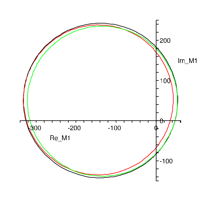


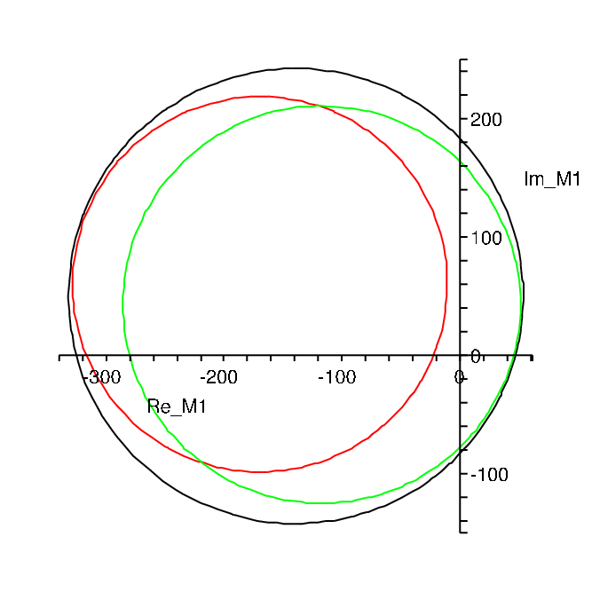


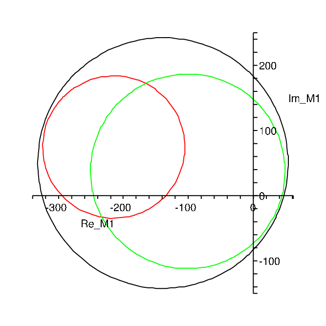


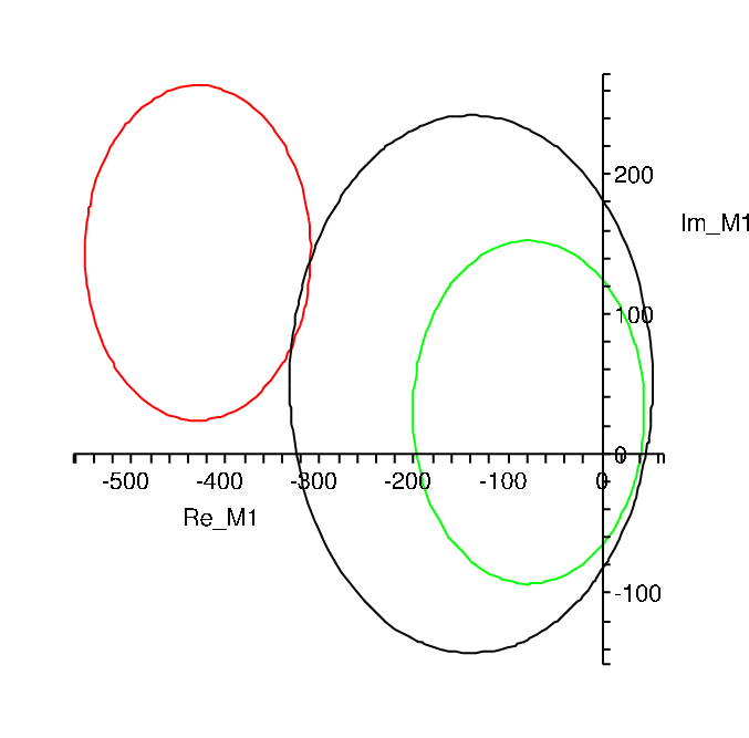


From these figures I conclude for the circle of the fourth neutralino:
- •
must be measured very precisely, small errors lead to large deviations from the unperturbed circle. The upper bound on this error is .
- •
The dependence on is weaker. A maximal error on about is allowed. The reason for the weak dependence is that does not depend on to zeroth order.
- •
The experimental error on should be small: . This is due to the strong dependence of on . For the error on its phase, I find: .
- •
For the error on , I find .
- •
The situation is similar or worse for the circles of the neutralinos and . For the circles of the second neutralino the influence of the error on is disastrous. I conclude that it is not possible to determine and with the circle method from Ref [40]. In the following section I propose an alternative method.
11 Determining Neutralino Couplings
I will show in this sections how radiative neutralino production together with neutralino pair production
| (95) |
can be used to determine the couplings of the neutralinos to the boson and to . My method is not only designed for the MSSM, it is applicable to every model with measurable cross sections. The idea is as follows: Write the cross section of an arbitrary process as
| (96) |
where the are functions of the unknown couplings , , and , the functions are not necessarily linear. The are calculable factors, depending only on the neutralino and selectron masses. If there are cross section measurements, number of couplings, then one can perform a least square fit to determine the couplings , , and . If the Eq. (96) is non-linear in the couplings one can either linearize Eq. (96) and use the custom linear least square functions provided by Maple or Mathematica or one can use techniques for non-linear fits like Minuit[119]. I have chosen the first approach because the linearized equations are not too complicated. The method is best illustrated by an example.
11.1 Mathematical Structure of the cross section and the couplings
To determine the couplings of the neutralinos to the selectrons and the -boson, I use the cross sections of the following reactions:
| (97a) | ||||
| (97b) | ||||
| (97c) | ||||
It is straightforward to include further reactions , , if they are measurable. Their cross sections can be decomposed as follows:
| (98a) | ||||
| (98b) | ||||
| (98c) | ||||
The factors , , are associated with the couplings to the right-selectron, left-selectron, and -boson, respectively, and are given by
| (99a) | ||||
| (99b) | ||||
| (99c) | ||||
| (99d) | ||||
appears only quadratically in Eq. (98a) and may be small, its error from a least square fit however may be large. The optimal value for can become negative, which is unphysical. Therefore, the use of instead of as a fit parameter secures the convergence of the iteration. Due to this problem, the value of is not used further. The , , are functions of the right selectron mass, left selectron mass, and -mass, respectively. They all depend on the neutralino masses, the center of mass energy and the longitudinal polarisation of the electron-positron-beam. Their explicit form can be found in [120]. They need to be calculated only once. So one does not have the problem that the iterations in the program that tries to find the minimum of does not converge due to errors occurring when integrating out the , , and by Monte Carlo integration.
This set of equations is nonlinear in the couplings parameters. The equations can be expanded in a Taylor series up to first order:
| (100) |
where is a vector, collecting the parameters , , . The linearized equations can be solved by a least square fit recursively. is a first guess of the solution.
From the parameters , , and one can determine the entries of the neutralino diagonalisation matrix .
| (101a) | ||||
| (101b) | ||||
| (101c) | ||||
| (101d) | ||||
| (101e) | ||||
| (101f) | ||||
| (101g) | ||||
| (101h) | ||||
| (101i) | ||||
| (101j) | ||||
Eqs. (101a)- (101b) are derived from Eqs. (99a)-(99b), and are obtained from the unitarity relation of the matrix ; , and are constructed in such a way, that is orthogonal to ; the elements , are calculated from and as well as the orthogonality relation . We use unitarity to calculate and , because this leads to a smaller error for these elements. The sign is choosen in such a way, that are orthogonal to .
11.2 The cross sections for Neutralino pair production
In Fig. 17, I show the cross sections for , and for cms - energies from - for three different polarisations: in Fig. 17(a), in Fig. 17(b), and in Fig. 17(c). The figures show, how suitable beam polarisation enhances cross sections. enhances , and , pair production compared to unpolarised beams, the opposite beam polarisation enhances radiative neutralino production, and and . In my example model which I will present below in detail, the is mainly bino () which couples mostly to right handed sleptons, the mainly wino () which couples preferably to left handed slepton; so cross sections with involved are enhanced by right handed beam polarisation, and cross sections with are enhanced by left handed beam polarisation.
Polarised beams are essential for the described method to determine parameters, since they enhance couplings either between right handed particles or left handed particles.


12 An example
12.1 The model
In order to demonstrate my method, I choose an example model with light neutralinos, so that at least the processes , , , and are kinematically accessible at the ILC and the cross sections exceed for both polarisations. The higgsino components of should not be too small, so that there might be a chance to determine the -- coupling.
The input data and the derived neutralino and selectron masses are listed in the first row of Tab. 7. For comparison I also list the values for the SPS1a scenario.
| my model | 165 | 82.5 | 230 | 75 | 11 | 76.3 | 136.8 | -239.2 | 273.2 | 117.3 | 171.3 |
| SPS1a | 192 | 102 | 352 | 100 | 10 | 99 | 175 | 348 | 369 | 145 | 204 |
In my model the cross section for the process is larger than for both beam polarisations and the cross section of the process is larger than for left beam polarisation. Therefore, I shall later present a study including these processes. The fairly light particle spectrum and, additionally, the large wino component in the latter process are the reasons for the large cross sections. I do not include them from the beginning.
With these values the neutralino diagonalisation matrix follows as
| (102) |
The neutralino couplings to , , and are listed in Tab. 8.
| couplings to | couplings to | couplings to |
|---|---|---|
I assume that eight cross section measurements of each process are available: Four different cms energies of the beam (, , , ) are combined with two different longitudinal beam polarisations and .
Each measurement has an error. The error on the cross sections consists of the statistical Poisson error and the systematic error. I consider only the statistical error. To simulate the statistical error on a measurement, I calculate the exact cross section and add a Gaussian distributed random number with zero mean and variance . The statistical error follows from
| (103) | |||||
| (104) |
with and denoting the integrated luminosity in and the number of events of the process, respectively. Eq. (12.1) accounts for the fact that the number of events for radiative neutralino production is calculated as the difference from all events ”photon plus missing energy” and the radiative neutrino background. Eq. (104) is the Poisson error for neutralino pair production.
The values for the cross sections and their errors are:
| (105) |
The values in brackets are not used for further calculations as they are too small. These input data from Tab. 105 lead to equations for fit parameters. The diagonalisation matrix has 16 entries, but only six of them are independent because of unitarity. There are ten relations between the matrix elements together with 13 equations from the fit parameters. The system is overdetermined. I choose the equations to determine the elements of the diagonalisation matrix such, that the error on the elements is as small as possible. In principle, unitarity can be tested by the first and the second column. So it can be tested if there is an additional singlino field.
For the couplings I get as a result of the least square fit:
| couplings to | couplings to | couplings to |
|---|---|---|
The obtained value is
| (106) |
With these data I get as a neutralino mixing matrix:
The error matrix shows that the bino and the wino components can be determined with high accuracy. The higgsino components have large(r) errors, especially the ones of the heavy neutralinos.
The parameters , , and follow from
| (116e) | ||||
| (116f) | ||||
| (116g) | ||||
I do not derive any value for because the result is not very reliable. The relative error on , , , and are about (error propagation in this sub-block), and together with the bad behaviour of the function near its poles this leads to a result with a large error.
12.2 How much does radiative neutralino production improve the measurements?
If I omit the data from the process , and repeat the calculation, then I get for the couplings the following result:
| couplings to | couplings to | couplings to |
|---|---|---|
The errors on the elements of the neutralino mixing matrix are increased by about a factor of . This leads to the following values of the gaugino parameters
| (117a) | ||||
| (117b) | ||||
| (117c) | ||||
The error on is five times larger than the error of the case that includes radiative neutralino production. The error on is enlarged only by a small amount and the error of is more than doubled.
Including the cross section of radiative neutralino production leads to smaller errors on , , and . So it is worthwhile to examine radiative neutralino production at a future linear collider.
12.3 The effect of including the production of further neutralino pairs
As I mentioned at the beginning of this section, the cross sections for
| (118) | |||||
| (119) |
can exceed , see Fig. 18.


These two processes introduce two further couplings, and , for their definition see Eq. (99c). They are not necessary for calculating the elements of the neutralino diagonalisation matrix and I do not use them for further calculations. Nevertheless, they provide useful information about signs, see the next subsection. , , and can be expressed as
| , | (120a) | |||
| , | (120b) | |||
| , | (120c) | |||
| (120d) | ||||
The additional processes reduce the errors on and , . As a consequence the errors on , , and are reduced by , respectively.
12.4 Resolving Ambiguities
The system of Eq. (97) has eight fix points. The starting point determines that fix point to which the iteration will converge. Some of these fix points do not fulfill the unitarity condition, so these points are to be discarded. The signs of is choosen as . With this choice the signs of , , are fixed, if the solution is physical. The other signs of are choosen such that the eigenvectors are orthogonal to each other.
12.5 Unitarity
Throughout this method, I assumed unitarity, which means that the neutralino system is complete. This assumption can be dropped to test if there is an additional singlino field [121]. The eigenvector of the first and the second neutralino are suitable candidates to test unitarity. But a detailed analysis is beyond the scope of this study.
12.6 Further Studies
The presented method can be extended to
- •
the MSSM with a violating gaugino sector,
- •
NMSSM to test unitarity,
- •
the chargino sector to determine the matrices.
- •
The circle method could be used for precision measurements of the chargino parameters.
13 Conclusion and Summary
In this chapter I presented a method to determine the -- and -- couplings.
- •
The method from [40] to determine does not work because the circles are too sensitive to errors of the input data.
- •
It is possible to determine the discussed couplings from the polarised cross sections of radiative neutralino production and neutralino pair production with errors . The masses of the neutralinos and the selectrons must be known from LHC/ILC measurements.
- •
From the couplings one can determine the neutralino diagonalisation matrix. The errors on the elements are about .
- •
From the neutralino diagonalisation matrix and the neutralino masses one can determine the neutralino mass matrix. The errors of , , and are about ). It is difficult to determine with my method.
- •
Omitting the cross sections of radiative neutralino productions enlarges the errors on , , and . Additional processes such as reduce the error on the corresponding couplings and on , , and .
- •
The differences to a global fit approach are as follows: In Fittino [113], the parameters , , , and are fitted directly to the data, and the couplings are obtained as a by-product. In Fittino, up to SUSY parameters can be fitted to cross sections, edge positions, branching fractions, cross sections times branching fractions and Standard Model parameters from LHC/ILC measurements. The authors recover and with absolute errors of the order , and with an absolute error of the order ( degrees of freedom).
In my method, the couplings are the fit parameters to cross sections from ILC measurements. From the couplings, I obtain , , and . The couplings enter the tree level cross sections of the considered particles, which are in my case neutralinos. I recover the input parameters of my model with absolute errors of the order ( degrees of freedom). The coupling independent terms of the cross sections need to be computed only once. The cross sections need not to be approximated as in Fittino. I do not fit all MSSM parameters to the cross sections. I assume that all masses are known from LHC/ILC measurements.
Chapter 6 Radiative Neutralino Production
Appendix 6.A Lagrangian and Couplings
Appendix 6.B Amplitudes for Radiative Neutralino Production
I define the selectron and boson propagators as
| (125) | |||||
| (126) |
The tree-level amplitudes for right selectron exchange in the -channel, see the diagrams 1-3 in Fig. 4, are
| (127) | |||||
| (128) | |||||
The amplitudes for -channel exchange, see the diagrams 4-6 in Fig. 4, are
| (130) | |||||
| (131) | |||||
In the photino limit, my amplitudes -, Eqs. (127)-(), agree with those given in Ref. [48].
The amplitudes for boson exchange, see the diagrams 7 and 8 in Fig. 4, are
Note that additional sign factors appear in the amplitudes - and -, compared to -. They stem from the reordering of fermionic operators in the Wick expansion of the matrix. For radiative neutralino production , such sign factors appear since the two external neutralinos are fermions.44 4 Note that in Ref. [54] the relative sign in the amplitudes for boson and -channel exchange is missing. For details see Refs. [38, 58]. In addition an extra factor 2 is obtained in the Wick expansion of the matrix, since the Majorana field contains both creation and annihilation operators. In my conventions I follow here closely Ref. [38]. Other authors take care of this factor by multiplying the vertex by a factor 2 already [1]. For more details of this subtlety, see Ref. [1].
The amplitudes for left selectron exchange, see the diagrams 9-14 in Fig. 4, are obtained from the amplitudes by substituting
| (135) |
For exchange in the -channel they read
| (136) | |||||
| (137) | |||||
The -channel exchange amplitudes are
| (139) | |||||
| (140) | |||||
Our amplitudes - agree with those given in Ref. [57, 58], however there is an obvious misprint in amplitude of Ref. [57]. In addition I have checked that the amplitudes for fulfill the Ward identity , as done in Refs. [54, 57]. I find for -channel exchange, for -channel exchange, for boson exchange, and analog relations for the exchange amplitudes.
Appendix 6.C Spin Formalism and Squared Matrix Elements
I include the longitudinal beam polarisations of electron, , and positron, , with in their density matrices
| (142) | |||||
| (143) |
where is the third Pauli matrix and and are the helicity indices of electron and positron, respectively. The squared matrix elements are then obtained by
| (144) | |||||
| (145) | |||||
| (146) |
where an internal sum over the helicities of the outgoing neutralinos, as well as a sum over the polarisations of the photon is included. Note that I suppress the electron and positron helicity indices of the amplitudes in the formulas (127)-(). The product of the amplitudes in Eqs. (144) and (145) contains the projectors
| (147) | |||||
| (148) |
The contraction with the density matrices of the electron and positron beams leads finally to
| (149) | |||||
| (150) |
In the squared amplitudes, I include the electron and positron beam polarisations in the coefficients
| (151) |
In the following I give the squared amplitudes , as defined in Eqs. (144) and (145), for and exchange. To obtain the corresponding squared amplitudes for exchange, one has to substitute
| (152) |
There is no interference between diagrams with and exchange, since I assume the high energy limit where ingoing particles are considered massless.
| (153) | |||||
| (154) | |||||
| (156) | |||||
| (157) | |||||
| (159) | |||||
| (160) | |||||
| (161) | |||||
| (162) | |||||
| (163) | |||||
| (164) | |||||
| (165) | |||||
| (166) | |||||
| (167) | |||||
| (168) | |||||
| (169) | |||||
| (170) | |||||
| (171) | |||||
| (172) | |||||
| (173) | |||||
| (174) | |||||
| (175) | |||||
| (176) | |||||
| (177) | |||||
| (178) | |||||
| (179) | |||||
| (180) | |||||
| (181) | |||||
| (182) | |||||
| (183) | |||||
| (184) | |||||
| (185) | |||||
| (186) | |||||
| (187) | |||||
| (188) | |||||
I have calculated the squared amplitudes with FeynCalc [122]. When integrating the squared amplitude over the phase space, see Appendix 9, the --interference terms cancel the --interference terms due to a symmetry in these channels, caused by the Majorana properties of the neutralinos [55]. Note that in principle also terms proportional to would appear in the squared amplitudes , due to the inclusion of the width to regularise the pole of the propagator . However, since this is a higher order effect which is small far off the resonance, I neglect such terms. In addition they would vanish after performing a complete phase space integration.
Chapter 7 Amplitudes for Radiative Neutrino Production
0.8 \SetWidth0.7
For radiative neutrino production
| (189) |
I define the and boson propagators as
| (190) | |||||
| (191) |
| Vertex | Factor |
|---|---|
| \SetScale1.25 \SetWidth0.7 | |
| \SetScale1.25 \SetWidth0.7 | |
| \SetScale1.25 \SetWidth0.7 |
The tree-level amplitudes for boson exchange, see the diagrams 1-3 in Fig. 19, are then
| (192) | |||||
| (193) | |||||
| (194) | |||||
with the parameter
| (195) |
The amplitudes for boson exchange, see diagrams 4 and 5 in Fig. 19, are
| (196) | |||||
| (197) |
with the parameters
| (198) |
I have checked that the amplitudes for fulfill the Ward identity . I find for exchange and for exchange.
Chapter 8 Amplitudes for Radiative Sneutrino Production
1.0 \SetWidth0.7
For radiative sneutrino production
| (214) |
I define the chargino and boson propagators as
| (215) | |||||
| (216) |
| Vertex | Factor |
|---|---|
| \SetScale1.25 \SetWidth0.7 | |
| \SetScale1.25 \SetWidth0.7 | |
| \SetScale1.25 \SetWidth0.7 |
The tree-level amplitudes for chargino exchange, see the contributing diagrams 1-3 in Fig. 20, are
| (217) | |||||
| (218) | |||||
| (219) | |||||
with the parameter defined in Eq. (195). The matrices and diagonalise the chargino mass matrix [1]
| (220) |
The amplitudes for chargino exchange, see the contributing diagrams 4-6 in Fig. 20, are
| (221) | |||||
| (222) | |||||
| (223) | |||||
The amplitudes for boson exchange, see the diagrams 7 and 8 in Fig. 20, read
| (224) | |||||
| (225) |
with the parameters , , and defined in Eq. (198). I have checked that the amplitudes , , fulfill the Ward identity , as done in Ref. [81]. I find for exchange, for exchange, and for boson exchange. Our amplitudes for chargino and boson exchange agree with those given in Refs. [81, 82], and in the limit of vanishing chargino mixing with those of Ref. [52]. However, there are obvious misprints in the amplitudes and of Ref. [82], see their Eqs. (7) and (9), respectively, and in the amplitude of Ref. [52], see their Eq. (F.3).
I then obtain the squared amplitudes and as defined in Eqs. (144) and (145):
| (226) | |||||
| (227) | |||||
| (228) | |||||
| (229) | |||||
| (230) | |||||
| (231) | |||||
| (232) | |||||
| (233) | |||||
| (234) | |||||
| (235) | |||||
| (236) | |||||
| (237) | |||||
| (238) | |||||
| (239) | |||||
| (240) | |||||
| (241) | |||||
| (242) | |||||
| (243) | |||||
| (244) | |||||
| (245) | |||||
| (246) | |||||
| (247) | |||||
| (248) | |||||
| (249) | |||||
| (250) | |||||
| (251) | |||||
| (252) | |||||
| (253) | |||||
| (254) | |||||
| (255) | |||||
| (256) | |||||
| (257) | |||||
| (258) | |||||
| (259) | |||||
| (260) | |||||
| (261) | |||||
Formulas for the squared amplitudes for radiative sneutrino production can also be found in Refs. [81, 82] for longitudinal and transverse beam polarisations. Here, I give however my calculated amplitudes for completeness. I have calculated the squared amplitudes with FeynCalc [122]. I neglect terms proportional to , see the discussion at the end of Appendix 6.
Chapter 9 Definition of the Differential Cross Section and Phase Space
I present some details of the phase space calculation for radiative neutralino production
| (262) |
The differential cross section for (262) is given by [123]
| (263) |
where and denote the final three-momenta and the final energies of the neutralinos and the photon. The squared matrix element is given in Appendix 6.
I parametrise the four-momenta in the center-of-mass (cms) system of the incoming particles, which I call the laboratory (lab) system. The beam momenta are then parametrised as
| (264) |
For the outgoing neutralinos and the photon I consider in a first step the local center-of-mass system of the two neutralinos. The photon shall escape along this -axis. I start with general momentum-vectors for the two neutralinos, boost them along their -axis and rotate them around the -axis to reach the lab system. Note that the three-momenta of the outgoing particles lie in a plane whose normal vector is inclined by an angle towards the beam axis. I parametrise the neutralino momenta in their cms frame [48]
| (265) |
with the local cms energy of the two neutralinos
| (266) |
the polar angle , the azimuthal angle and the absolute value of the neutralino three-momenta in their cms frame. These momenta are boosted to the lab system with the Lorentz transformation
| (267) |
with and the boost velocity from the cms to the lab system
| (268) |
Boosting the momenta and , see Eq. (265), at first with the Lorentz transformation Eq. (267) and then rotating with yields the neutralino and photon momenta in the lab system [48]
| (269) | |||||
| (270) | |||||
| (271) |
with
| (272) | |||||
| (273) | |||||
| (274) |
The differential cross section for now reads [48]
| (275) |
where the integration variables run over
| (276) |
Chapter 10 How to calculate helicity amplitudes for longitudinal polarisation states
Appendix 10.A Introduction
Bouchiat and Michel presented [124] formulae to perform helicity spin sums for Dirac fermions and antifermions. Haber collected in [125] mathematical tools to deal with such sums and presented example calculations. Choi et al.[126] extended these formulae to spin 1 and spin fields. In this paper I present a proof of the Bouchiat-Michel-formulae and I extend these formulae to Majorana particles. All formulae are written in a covariant manner.
Appendix 10.B Spinor calculus
The Dirac spinors and obey the Dirac equation:
| (277) |
The charge-conjugation-operator converts the spinor with positive energy into the spinor with negative energy and vice versa:
| (278) |
There are two solutions of the Dirac equations for a given 4-momentum , so there exists another good quantum number to label these states. This is the helicity . The helicity operator commutes with the Dirac operator , so the eigenvalues of are good quantum numbers.
The spinors and are normalized to ([127])
| (279) | |||||
| (280) |
When calculating cross sections or decay widths of fermions and antifermions, I sum over all spins states and average over initial spins, using the completeness relation [127]:
| (281) | |||||
| (282) |
When describing spin-polarized fermion ensemble one introduces spin vectors. The longitudinal spin vector for a particle with mass is defined by
| (283) |
is normalized to , and is orthogonal to the momentum vector : .
I have to do distinguish between massive and massless particles. The spinvector for massless particles is obtained in the limit .
10.B.1 The massive case
The operator commutes with , so both operators can be diagonalized simultaneously. Their eigenvectors are known, and the eigenvalues are obtained by [128] :
| (284) | |||||
I have used the relation to realize that is the helicity operator.
From the above calculation it follows immediately:
| (285) |
10.B.2 The massless case
The Dirac equation for a massless spin -fermion is:
| (286) |
and multiply eq. (286) with [128]:
| (287) | |||||
| (288) |
with . The chirality-operator commutes with the helicity-operator, hence they have common eigenvectors, a similar equation holds for spinors:
| (289) | |||||
| (290) |
Since , the eigenvalues of the chirality-operator are .
Appendix 10.C The Bouchiat-Michel-Formula
The Bouchiat-Michel-formulae (BMF) tell us how to contract spinors with different polarisations. The BMF is interesting if the initial state fermions have the same mass, but also in using density matrix techniques [125].
10.C.1 Spin vectors
I enlarge the set , defined in sec. 10.B with two other four-vectors and to a orthonormal basis in space-time:
| (291) | |||||
| (292) | |||||
| (293) |
with , .
The spinors , satisfy:
| (294) | |||
| (295) |
The proof of this equation can be found in/follows [129]: Define the Pauli-Lubanski-vector as
| (296) | |||||
| (297) |
where , , are the generators of the Poincare-group. In the rest frame the spin vectors take a simple form: where is the ith unit vector. I build the scalar operator , which has the eigenvalues and evaluate it in the rest frame:
| (298) |
Then, I apply on a spinor :
| (299) |
On the other hand , so
| (300) | |||||
Now eq. (294) follows. The proof for the spinor is similar.
10.C.2 BMF for massive Dirac fermions
Now I have all ingredients to formulate and prove the BMF:
| (301) | |||||
| (302) |
The sum must have the form
| (303) |
To determine the unknown coefficients , we multiply both sides with and with :
| (304) | |||||
A similar proof holds for eq. (302)
10.C.3 BMF for massless Dirac fermions
10.C.4 Majorana-Fermions
In supersymmetric (SUSY) field theories there appear Majorana fermions, for example the neutralinos, which are the SUSY partners of the neutral weak gauge and Higgs bosons. In Feynman diagrams with Majorana fermions I find often clashing arrows. So it is useful to have formulae to handle this case. I use the relations (278), and I get
Appendix 10.D Calculation of the density matrix
The methods described above can be used to compute squared matrix elements in the helicity mechanism described in [125]. The only change in the usual mechanism is the completeness relation. I consider longitudinal polarized electrons. I treat the electrons as massless. I call this matrix the reaction matrix .
| (312) |
References
- [1] H. E. Haber and G. L. Kane, Phys. Rept. 117, 75 (1985).
- [2] I. J. R. Aitchison, arXiv:hep-ph/0505105.
- [3] M. Drees, arXiv:hep-ph/9611409.
- [4] M. Drees, R. M. Godbole, and P. Roy. Theory and Phenomenology of Sparticles”. (World Scientific, 2005.)
- [5] H. P. Nilles, Phys. Rept. 110 (1984) 1.
- [6] R. A. Horn and C. R. Johnson “Matrix Analysis”. (Cambridge University Press, 1985.)
- [7] M. M. El Kheishen, A. A. Aboshousha and A. A. Shafik, Phys. Rev. D 45 (1992) 4345.
- [8] J. F. Gunion and H. E. Haber, Phys. Rev. D 37 (1988) 2515.
- [9] I. Gogoladze, J. D. Lykken, C. Macesanu and S. Nandi, Phys. Rev. D 68 (2003) 073004 [arXiv:hep-ph/0211391]; V. Barger, P. Langacker and H. S. Lee, Phys. Lett. B 630 (2005) 85 [arXiv:hep-ph/0508027].
- [10] D. Choudhury, H. K. Dreiner, P. Richardson and S. Sarkar, Phys. Rev. D 61, 095009 (2000) [arXiv:hep-ph/9911365].
- [11] W. M. Yao et al. [Particle Data Group], J. Phys. G 33 (2006) 1.
- [12] J. Abdallah et al. [DELPHI Collaboration], Eur. Phys. J. C 31 (2004) 421 [arXiv:hep-ex/0311019].
- [13] D. N. Spergel et al. [WMAP Collaboration], Astrophys. J. Suppl. 148 (2003) 175 [arXiv:astro-ph/0302209].
- [14] E. W. Kolb, M. T. Turner “The Early Universe .” (Westview Press 1990.)
- [15] K. Griest and D. Seckel, Phys. Rev. D 43 (1991) 3191.
- [16] H. K. Dreiner, arXiv:hep-ph/9707435.
- [17] S. S. Gershtein and Y. B. Zeldovich, JETP Lett. 4 (1966) 120 [Pisma Zh. Eksp. Teor. Fiz. 4 (1966) 174].
- [18] R. Cowsik and J. McClelland, Phys. Rev. Lett. 29 (1972) 669.
- [19] B. W. Lee and S. Weinberg, Phys. Rev. Lett. 39 (1977) 165.
- [20] P. Hut, Phys. Lett. B 69 (1977) 85.
- [21] K. Sato and M. Kobayashi, Prog. Theor. Phys. 58 (1977) 1775.
- [22] M. I. Vysotsky, A. D. Dolgov and Y. B. Zeldovich, JETP Lett. 26 (1977) 188 [Pisma Zh. Eksp. Teor. Fiz. 26 (1977) 200].
- [23] A. Bottino, F. Donato, N. Fornengo and S. Scopel, Phys. Rev. D 68 (2003) 043506 [arXiv:hep-ph/0304080].
- [24] P. Gondolo and G. Gelmini, Nucl. Phys. B 360 (1991) 145.
- [25] C. L. Bennett et al., Astrophys. J. Suppl. 148 (2003) 1 [arXiv:astro-ph/0302207].
- [26] H. K. Dreiner, C. Luhn and M. Thormeier, Phys. Rev. D 73 (2006) 075007 [arXiv:hep-ph/0512163].
- [27] G. Belanger, F. Boudjema, A. Pukhov and A. Semenov, Comput. Phys. Commun. 174 (2006) 577 [arXiv:hep-ph/0405253].
- [28] D. Hooper and T. Plehn, Phys. Lett. B 562 (2003) 18 [arXiv:hep-ph/0212226].
- [29] G. Belanger, F. Boudjema, A. Cottrant, A. Pukhov and S. Rosier-Lees, JHEP 0403 (2004) 012 [arXiv:hep-ph/0310037].
- [30] G. Abbiendi et al. [OPAL Collaboration], Eur. Phys. J. C 35 (2004) 1 [arXiv:hep-ex/0401026].
- [31] J. F. Gunion and H. E. Haber, Nucl. Phys. B 272 (1986) 1 [Erratum-ibid. B 402 (1993) 567].
- [32] J. A. Aguilar-Saavedra et al. [ECFA/DESY LC Physics Working Group], arXiv:hep-ph/0106315.
- [33] T. Abe et al. [American Linear Collider Working Group], arXiv:hep-ex/0106055.
- [34] K. Abe et al. [ACFA Linear Collider Working Group], arXiv:hep-ph/0109166.
- [35] G. Weiglein et al. [LHC/LC Study Group], arXiv:hep-ph/0410364.
- [36] J. A. Aguilar-Saavedra et al., Eur. Phys. J. C 46 (2006) 43 [arXiv:hep-ph/0511344].
- [37] G. A. Moortgat-Pick et al., arXiv:hep-ph/0507011.
- [38] A. Bartl, H. Fraas and W. Majerotto, Nucl. Phys. B 278 (1986) 1.
- [39] The original computations of neutralino pair production at -colliders include: with mixing, but with simplifications in the masses: J. R. Ellis, J. M. Frere, J. S. Hagelin, G. L. Kane and S. T. Petcov, Phys. Lett. B 132 (1983) 436; with pure Zino production: E. Reya, Phys. Lett. B 133 (1983) 245; with partial neutralino mixing: P. Chiappetta, J. Soffer, P. Taxil, F. M. Renard and P. Sorba, Nucl. Phys. B 262 (1985) 495 [Erratum-ibid. B 279 (1987) 824]. The first complete computation is given in Ref. [38].
- [40] S. Y. Choi, J. Kalinowski, G. A. Moortgat-Pick and P. M. Zerwas, Eur. Phys. J. C 22, 563 (2001) [Addendum-ibid. C 23, 769 (2002)] [arXiv:hep-ph/0108117].
- [41] S. Y. Choi, B. C. Chung, J. Kalinowski, Y. G. Kim and K. Rolbiecki, Eur. Phys. J. C 46 (2006) 511 [arXiv:hep-ph/0504122].
- [42] V. D. Barger, T. Han, T. J. Li and T. Plehn, Phys. Lett. B 475 (2000) 342 [arXiv:hep-ph/9907425].
- [43] J. L. Kneur and G. Moultaka, Phys. Rev. D 61, 095003 (2000) [arXiv:hep-ph/9907360].
- [44] H. Goldberg, Phys. Rev. Lett. 50 (1983) 1419.
- [45] J. R. Ellis, J. S. Hagelin, D. V. Nanopoulos, K. A. Olive and M. Srednicki, Nucl. Phys. B 238 (1984) 453.
- [46] P. Fayet, Phys. Lett. B 117 (1982) 460.
- [47] J. R. Ellis and J. S. Hagelin, Phys. Lett. B 122 (1983) 303.
- [48] K. Grassie and P. N. Pandita, Phys. Rev. D 30, 22 (1984).
- [49] T. Kobayashi and M. Kuroda, Phys. Lett. B 139 (1984) 208.
- [50] J. D. Ware and M. E. Machacek, Phys. Lett. B 142 (1984) 300.
- [51] L. Bento, J. C. Romao and A. Barroso, Phys. Rev. D 33 (1986) 1488.
- [52] M. Chen, C. Dionisi, M. Martinez and X. Tata, Phys. Rept. 159 (1988) 201.
- [53] T. Kon, Prog. Theor. Phys. 79 (1988) 1006.
- [54] M. Bayer, Diploma thesis, “Radiative Erzeugung von Neutralinos durch Vernichtung polarisierter Elektron-Positron-Strahlen”, University of Würzburg, Germany (1992).
- [55] S. Y. Choi, J. S. Shim, H. S. Song, J. Song and C. Yu, Phys. Rev. D 60 (1999) 013007 [arXiv:hep-ph/9901368].
- [56] H. Baer and A. Belyaev, “Associated neutralino neutralino photon production at NLC,” in Proc. of the APS/DPF/DPB Summer Study on the Future of Particle Physics (Snowmass 2001) ed. N. Graf, eConf C010630 (2001) P336 [arXiv:hep-ph/0111017].
- [57] M. Weidner, Diploma thesis, “Radiative Erzeugung von Neutralinos in Elektron-Positron-Kollisionen”, University of Würzburg, Germany (2003).
- [58] H. Fraas and H. Wolter, “Radiative production of the lightest neutralino in annihilation,” PRINT-91-0421 (WURZBURG).
- [59] A. Datta, A. Datta and S. Raychaudhuri, Phys. Lett. B 349 (1995) 113 [arXiv:hep-ph/9411435].
- [60] A. Datta, A. Datta and S. Raychaudhuri, Eur. Phys. J. C 1 (1998) 375 [arXiv:hep-ph/9605432].
- [61] A. Datta and A. Datta, Phys. Lett. B 578 (2004) 165 [arXiv:hep-ph/0210218].
- [62] S. Ambrosanio, B. Mele, G. Montagna, O. Nicrosini and F. Piccinini, Nucl. Phys. B 478 (1996) 46 [arXiv:hep-ph/9601292].
- [63] A. I. Ahmadov, Phys. Atom. Nucl. 69 (2006) 51.
- [64] A. I. Ahmadov, Phys. Part. Nucl. Lett. 2 (2005) 85 [Pisma Fiz. Elem. Chast. Atom. Yadra 2 (2005) 34].
- [65] C. H. Chen, M. Drees and J. F. Gunion, Phys. Rev. Lett. 76 (1996) 2002 [arXiv:hep-ph/9512230]; Erratum arXiv:hep-ph/9902309.
- [66] G. L. Kane and G. Mahlon, Phys. Lett. B 408 (1997) 222 [arXiv:hep-ph/9704450].
- [67] A. Datta and S. Maity, Phys. Rev. D 59 (1999) 055019 [arXiv:hep-ph/9808423].
- [68] G. Abbiendi et al. [OPAL Collaboration], Eur. Phys. J. C 29 (2003) 479 [arXiv:hep-ex/0210043].
- [69] A. Birkedal, K. Matchev and M. Perelstein, Phys. Rev. D 70 (2004) 077701 [arXiv:hep-ph/0403004].
- [70] A. Heister et al. [ALEPH Collaboration], Eur. Phys. J. C 28 (2003) 1.
- [71] J. Abdallah et al. [DELPHI Collaboration], Eur. Phys. J. C 38, 395 (2005) [arXiv:hep-ex/0406019].
- [72] P. Achard et al. [L3 Collaboration], Phys. Lett. B 587 (2004) 16 [arXiv:hep-ex/0402002].
- [73] G. Abbiendi et al. [OPAL Collaboration], Eur. Phys. J. C 18 (2000) 253 [arXiv:hep-ex/0005002].
- [74] K. J. F. Gaemers, R. Gastmans and F. M. Renard, Phys. Rev. D 19, 1605 (1979).
- [75] D. Choudhury, H. K. Dreiner, P. Richardson and S. Sarkar, Phys. Rev. D 61 (2000) 095009 [arXiv:hep-ph/9911365]; A. Dedes, H. K. Dreiner and P. Richardson, Phys. Rev. D 65 (2002) 015001 [arXiv:hep-ph/0106199]; H. K. Dreiner, C. Hanhart, U. Langenfeld and D. R. Phillips, Phys. Rev. D 68 (2003) 055004 [arXiv:hep-ph/0304289].
- [76] M. Gataullin [LEP Collaboration], Eur. Phys. J. C 33, S791 (2004) [arXiv:hep-ex/0311014].
- [77] E. Boos et al. [CompHEP Collaboration], Nucl. Instrum. Meth. A 534 (2004) 250 [arXiv:hep-ph/0403113].
- [78] F. A. Berends, G. J. H. Burgers, C. Mana, M. Martinez and W. L. van Neerven, Nucl. Phys. B 301, 583 (1988).
- [79] F. Boudjema et al., arXiv:hep-ph/9601224.
- [80] G. Montagna, M. Moretti, O. Nicrosini and F. Piccinini, Nucl. Phys. B 541 (1999) 31 [arXiv:hep-ph/9807465].
- [81] F. Franke, Diploma thesis, “Radiative Erzeugung skalarer Neutrinos in Elektron-Positron-Kollisionen”, University of Würzburg, Germany (1992).
- [82] F. Franke and H. Fraas, Phys. Rev. D 49 (1994) 3126.
- [83] N. Ghodbane and H. U. Martyn, in Proc. of the APS/DPF/DPB Summer Study on the Future of Particle Physics (Snowmass 2001) ed. N. Graf, arXiv:hep-ph/0201233.
- [84] B. C. Allanach et al., in Proc. of the APS/DPF/DPB Summer Study on the Future of Particle Physics (Snowmass 2001) ed. N. Graf, Eur. Phys. J. C 25 (2002) 113 [eConf C010630 (2001) P125] [arXiv:hep-ph/0202233].
- [85] H. E. Haber and D. Wyler, Nucl. Phys. B 323 (1989) 267.
- [86] S. Ambrosanio and B. Mele, Phys. Rev. D 53 (1996) 2541 [arXiv:hep-ph/9508237].
- [87] S. Ambrosanio and B. Mele, Phys. Rev. D 55, 1399 (1997) [Erratum-ibid. D 56, 3157 (1997)] [arXiv:hep-ph/9609212].
- [88] H. Baer and T. Krupovnickas, JHEP 0209, 038 (2002) [arXiv:hep-ph/0208277].
- [89] LEP SUSY Working group, LEPSUSYWG/02-06.2; G. Ganis [ALEPH Collaboration], ALEPH-2000-065 Prepared for 30th International Conference on High-Energy Physics (ICHEP 2000), Osaka, Japan, 27 Jul - 2 Aug 2000
- [90] L. E. Ibanez and C. Lopez, Nucl. Phys. B 233 (1984) 511.
- [91] L. E. Ibanez, C. Lopez and C. Munoz, Nucl. Phys. B 256 (1985) 218.
- [92] L. J. Hall and J. Polchinski, Phys. Lett. B 152 (1985) 335.
- [93] A. Vest, LC-TH-2000-058, in 2nd ECFA/DESY Study 1998-2001, 1326.
- [94] T. Ohl, Comput. Phys. Commun. 101 (1997) 269 [arXiv:hep-ph/9607454].
- [95] A. Hinze, LC-PHSM-2005-001.
- [96] A. Bartl, K. Hidaka, T. Kernreiter and W. Porod, Phys. Rev. D 66 (2002) 115009 [arXiv:hep-ph/0207186].
- [97] S. K. Soni and H. A. Weldon, Phys. Lett. B 126 (1983) 215.
- [98] See the summary talk of the polarization parallel session by Sabine Riemann given at the ILC conference in Valencia, 5-13 November 2006. http://ific.uv.es/ ilc/ECFA-GDE2006/
- [99] See the talk by Gudrid Moortgat-Pick in the polarization parallel session at the ILC conference in Valencia, 5-13 November 2006. http://ific.uv.es/ ilc/ECFA-GDE2006/
- [100] See the talk by Erez Reinherz-Aronis in the polarization parallel session at the ILC conference in Valencia, 5-13 November 2006. http://ific.uv.es/ ilc/ECFA-GDE2006/
- [101] See, e.g., G. Moortgat-Pick, arXiv:hep-ph/0607173.
- [102] H. K. Dreiner, O. Kittel and U. Langenfeld, Phys. Rev. D 74 (2006) 115010 [arXiv:hep-ph/0610020].
- [103] M. T. Dova, P. Garcia-Abia and W. Lohmann, arXiv:hep-ph/0302113.
- [104] Moenig et al.
- [105] I. Borjanovic et al., Eur. Phys. J. C 39S2 (2005) 63 [arXiv:hep-ex/0403021].
- [106] M. Martinez and R. Miquel, Eur. Phys. J. C 27 (2003) 49 [arXiv:hep-ph/0207315].
- [107] A. H. Chamseddine, R. Arnowitt and P. Nath, Phys. Rev. Lett. 49 (1982) 970; P. Nath, R. Arnowitt and A. H. Chamseddine, Nucl. Phys. B 227 (1983) 121. For a review see also [5].
- [108] W. Porod, Comput. Phys. Commun. 153 (2003) 275 [arXiv:hep-ph/0301101].
- [109] S. Y. Choi, A. Djouadi, M. Guchait, J. Kalinowski, H. S. Song and P. M. Zerwas, Eur. Phys. J. C 14 (2000) 535 [arXiv:hep-ph/0002033].
- [110] K. Desch, J. Kalinowski, G. A. Moortgat-Pick, M. M. Nojiri and G. Polesello, JHEP 0402 (2004) 035 [arXiv:hep-ph/0312069].
- [111] P. Bechtle, K. Desch, W. Porod and P. Wienemann, Eur. Phys. J. C 46 (2006) 533 [arXiv:hep-ph/0511006].
- [112] P. Bechtle, K. Desch and P. Wienemann, arXiv:hep-ph/0511137.
- [113] P. Bechtle, K. Desch and P. Wienemann, Comput. Phys. Commun. 174 (2006) 47 [arXiv:hep-ph/0412012].
- [114] K. Madsen, H. B. Nielsen, O. Tiengleff. Methods for non-linear least square problems. April 2004. Informatics and Methematical Modelling, Technical University of Denmark.
- [115] K. Desch, J. Kalinowski, G. Moortgat-Pick, K. Rolbiecki and W. J. Stirling, JHEP 0612 (2006) 007 [arXiv:hep-ph/0607104].
- [116] R. Lafaye, T. Plehn and D. Zerwas, arXiv:hep-ph/0404282.
- [117] C. G. Lester, M. A. Parker and M. J. White, JHEP 0601 (2006) 080 [arXiv:hep-ph/0508143].
- [118] B. C. Allanach, D. Grellscheid and F. Quevedo, JHEP 0407 (2004) 069 [arXiv:hep-ph/0406277].
- [119] F. James, “Minuit. Function Minimization and Error Analysis. Computing and Network Division CERN.”
- [120] G. A. Moortgat-Pick, H. Fraas, A. Bartl and W. Majerotto, Eur. Phys. J. C 9, 521 (1999) [Erratum-ibid. C 9, 549 (1999)] [arXiv:hep-ph/9903220].
- [121] U. Ellwanger, M. Rausch de Traubenberg and C. A. Savoy, Nucl. Phys. B 492 (1997) 21 [arXiv:hep-ph/9611251].
- [122] J. Kublbeck, H. Eck and R. Mertig, Nucl. Phys. Proc. Suppl. 29A (1992) 204, http://www.feyncalc.org.
- [123] S. Eidelman et al. [Particle Data Group], Phys. Lett. B 592 (2004) 1.
- [124] C. Bouchiat and L. Michel, Nucl. Phys. 5 (1958) 416.
- [125] H. E. Haber, arXiv:hep-ph/9405376.
- [126] S. Y. Choi, T. Lee, and H. S. Song, Phys. Rev. D 40 (1989) 2477.
- [127] M. E. Peskin, D. V. Schroeder “An Introduction to Quantum Field Theory”. (Perseus Books, Cambridge, MA 1995.)
- [128] F. Schwabl, “QM II”. (Springer, Berlin 2000.)
- [129] D. Bailin “Weak Interactions”. (Sussex University Press 1977.)
- [130] LEPSUSYWG, ALEPH, DELPHI, L3 and OPAL experiments, note LEPSUSYWG/01-03.1 (http://lepsusy.web.cern.ch/lepsusy/Welcome.html).
- [131] A. Bartl, H. Fraas, W. Majerotto and N. Oshimo, Phys. Rev. D 40 (1989) 1594.
- [132] M. Dittmar and H. K. Dreiner, Phys. Rev. D 55 (1997) 167 [arXiv:hep-ph/9608317]; M. Dittmar and H. K. Dreiner, arXiv:hep-ph/9703401.