Shear viscosity of a superfluid Fermi gas in the unitarity limit
Abstract
We compute the shear viscosity of a superfluid atomic Fermi gas in the unitarity limit. The unitarity limit is characterized by a divergent scattering length between the atoms, and it has been argued that this will result in a very small viscosity. We show that in the low temperature limit the shear viscosity scales as , where the universal parameter relates the chemical potential and the Fermi energy, . Combined with the high temperature expansions of the viscosity our results suggest that the viscosity has a minimum near the critical temperature . A naïve extrapolation indicates that the minimum value of the ratio of viscosity over entropy density is within a factor of of the proposed bound .
I introduction
Shear viscosity can be defined as the shearing force per unit area per unit velocity gradient in a laminar flow. For a flow in -direction, with a velocity gradient in the -direction
| (1) |
Viscosity relates the rate of momentum transfer to the velocity gradient. For dilute gases the microscopic mechanism for momentum transfer is provided by atomic collisions. This mechanism becomes more efficient as the mean free path gets larger because in that case the atoms travel larger distances between collisions and transfer momenta between laminar layers of more disparate flow velocities. Thus viscosity is expected to be inversely proportional to the collision cross section . This leads to the question of whether there is a fundamental limit to how small the viscosity can get as the strength of the interaction is increased. Stated differently, we would like to determine the shear viscosity of the most “perfect” fluid.
There is an old argument that suggests that quantum mechanics places a lower limit on the shear viscosity Danielewicz:1984ww. A rough estimate of the viscosity is provided by , where is the number density, is the average momentum, and the mean free-path. Heisenberg’s uncertainty principle requires and the kinematic viscosity . For relativistic systems particle number is not conserved and it is more natural to consider , where is the entropy density. As long as the entropy per particle is of the order we expect .
A new perspective on this idea is provided by a calculation, based on the AdS/CFT correspondence, of in the strong coupling limit of super-symmetric Yang Mills theory Policastro:2001yc. This calculation gives , a value that is also obtained in other strongly coupled field theories that have a gravity dual. It is also known that the leading order correction to the limit of infinite coupling increases . This has led to the conjecture that the strong coupling result is a universal lower bound for all fluids Kovtun:2004de:
| (2) |
Liquid Helium comes to within an order of magnitude of the bound, and values have been reported for the quark gluon plasma produced at RHIC Teaney:2003kp; Hirano:2005wx. There are suggestions in the literature that counter examples can be found by considering non-relativistic systems for which the entropy per particle is very large Cohen:2007qr; Dobado:2007tm, but currently no fluid that violates the bound is experimentally known.
An interesting system to study in this context is a cold atomic gas near a Feshbach resonance JEThomas; TBourdel; KDieckmann; DJin; SJochim. In 6Li and 40K gases, there exist hyperfine channels that support bound states. The magnetic moment of the bound state in these channels is different from the sum of the magnetic moments of the atoms that make the bound state. This allows one to use an external magnetic field to move the bound state energy relative to the continuum states, effectively making the bound state arbitrarily shallow. In terms of scattering theory, a shallow bound state corresponds to a large scattering length. At the Feshbach resonance, the atomic cross section is only limited by unitarity . The unitarity gas interaction is characterized by a divergent two-body scattering length and a natural sized range . Even for a dilute gas with density , the unitarity gas with is a strongly interacting system. In fact it is the most strongly interacting non-relativistic system known, with a diverging two-body collision cross section .
The aim in this work is to improve the understanding of transport properties of the cold unitarity gas by performing a systematic calculation of the shear viscosity in the low temperature superfluid phase. Combined with known results in the high temperature limit Bruun these results provide an estimate of the minimum viscosity. In the superfluid phase Cooper pairs break the symmetry associated with the conservation of particle number. This implies that there is a Nambu-Goldstone boson, the phonon. At temperatures below the critical temperature for superfluidity, phonons dominate thermodynamic and transport properties of the system.
The paper is organized as follows. In Section II we present the basic equations relating the shear viscosity to the phonon collision operator. The phonon interaction is derived in Section III, followed by a variational calculation of the viscosity in Section IV. A discussion of the result is presented. The discussion closely parallels the calculation of the viscosity in liquid Helium Khalatnikov; Maris and, in particular, the CFL phase of dense quark matter Manuel:2004iv. We end with the conclusions in Section V.
II Transport Equation and Viscosity
Viscosity as defined in Eq. (1) is related to internal stresses in a fluid. A more convenient definition is provided by the stress-energy tensor of an almost ideal fluid. Close to equilibrium it can be expanded in derivatives of the flow velocity ,
| (3) | ||||
where we only kept the traceless part of . The trace of is related to bulk viscosity. The ideal fluid part of is related to the thermodynamic variables pressure and energy density . In the superfluid phase the long distance fluctuations of the order parameters and of the conserved quantities are described by the two-fluid hydrodynamics. The two components are a non-viscous superfluid, and a viscous normal fluid. The stress-energy tensor of the normal fluid is given by Eq. (3), where is now the velocity of the normal fluid.
If the normal fluid is composed of weakly interacting quasi-particles the stress-energy tensor and the viscosity can be computed using kinetic theory. In the unitarity Fermi gas at very low temperature the quasi-particles are the phonons. The stress-energy tensor is given by Landau
| (4) |
where is the distribution function of the phonons with speed , momenta and energy . Close to the equilibrium , where is the Bose-Einstein distribution and is a small departure from equilibrium. Small fluctuations can be parameterized in terms of departures of the thermodynamics variables from equilibrium, e.g. . This motivates the definition in terms of the unknown function . To project onto the shear stress, one uses the ansatz
| (5) |
where only the traceless projection on the momenta is relevant. Thus close to the equilibrium one can write
| (6) | ||||
This determines the shear viscosity in terms of the function ,
| (7) | ||||
The equation of motion for is derived using the Boltzmann equation
| (8) |
relating the rate of change of the distribution function to the collision operator . In the absence of external force we take . The left hand side of the relation Eq. (8) can be simplified further Landau to write:
| (9) | ||||
where only the contribution relevant for shear viscosity was retained in the Linear Response Approximation, leading order in the small deviation from equilibrium.
Two types of contributions to the collision term are typically considered: binary collisions in which the number of particles is conserved, and “splitting” processes in which the number of particles is not conserved. These processes are shown in Fig. 1. We will show in Section III that splitting processes do not contribute to shear viscosity at leading order in the low temperature approximation.

The collision integral is given by
| (10) | ||||
where contains the distribution functions and is the scattering amplitude shown in Fig. 1. The distribution functions are linearized in the small deviations from the equilibrium distribution, . We find:
| (11) | ||||
where we have used the equilibrium relation
| (12) |
This relation ensures that and in thermal equilibrium.
Using the ansatz in Eq. (5) for , we get
| (13) | ||||
where we have defined the linearized collision operator . We have also defined
| (14) | ||||
Using Eqs. (8), (9) and (13), the linearized Boltzmann equation can be written as
| (15) |
This result can be used to rewrite the relation for the viscosity in Eq. (7) as
| (16) |
which will be useful later. We used the linear dispersion relation above, sufficient for the calculation as shown in the next section. To complete the calculation of the solution to the collision equation we need to calculate the scattering amplitude which we will turn to now.
III Phonon Cross Section
The phonon interaction for the unitarity gas in the superfluid phase can be derived from Galilean and gauge invariance Greiter:1989qb; Son:2005rv. Consider a microscopic Lagrangian for the unitarity Fermi gas
| (17) |
where is two component spinor, is the mass of the Fermion, is the anti-symmetric Pauli matrix, and is an interaction strength that can be tuned to achieve infinite scattering length. This Lagrangian is invariant under Galilean transformations, and under the gauge transformation where the fictitious gauge field is defined as . We work in units where .
We require that the effective theory for the phonon field shares the symmetries of the microscopic Lagrangian. This implies that the effective Lagrangian is a function of
| (18) |
and its derivatives Son:2002zn; Son:2005rv. The functional dependence on is further restricted by the observation that the effective action at its minimum , for constant classical field , is equal to the pressure of the unitarity gas. In the limit , which is nearly realized in cold atomic traps JEThomas; TBourdel; KDieckmann; DJin; SJochim, the unitarity gas is a scale invariant system. This implies that, up to a numerical constant, the pressure has to be equal to that of the free system. We write
| (19) |
where the universal constant is sometimes called the Bertsch parameter in the nuclear physics community. Eq. (19) implies , where , , and is the number density. We conclude that Son:2005rv
| (20) | ||||
where corresponds to terms with derivatives of . We can bring the kinetic term into the canonical form via a field rescaling . We find expanding in derivatives of the phonon field, ignoring total derivatives of the dynamical field and constants independent of ,
| (21) | ||||
where and the Nambu-Goldstone boson speed is .
The determination of is a non-perturbative many-body problem, and there are no exact analytical calculation available. Numerical calculations using fixed node Green’s Function Monte Carlo Carlson2003; Chang2004; Astrakharchik2004 or Euclidean lattice calculations Chen:2003vy; Lee:2005fk; Bulgac:2005pj; Burovski:2006 find . Our final result depends on this single universal number .
We can estimate the sizes of the different terms in the Lagrangian as follows: for the kinetic term to contribute to the generating functional its contribution should be otherwise it will be damped in the exponential. Time derivatives scale as , spatial derivatives as , and the volume integral scales as . This implies that . We observe that the magnitude of the phonon self coupling relative to the kinetic term scales as , a small correction for . Note that for a strongly interacting unitarity gas TC for , which implies that is of the order .
The Lagrangian in Eq. (21) describes the leading order phonon interaction for the processes shown in Fig. 1. At this order, the phonon dispersion relation is linear with . Consequently, the splitting processes are collinear and cannot contribute to the shear viscosity.
Binary Collisions
The leading order contribution to the binary collision processes in Fig. 1 are shown in Fig. 2. The contribution of the four-phonon contact term to the scattering amplitude is
| (22) |
where we have used and defined , and . We also assumed that the phonons are on-shell and that the dispersion relation is linear, . Factors of from Bose symmetry have been included in the amplitudes.
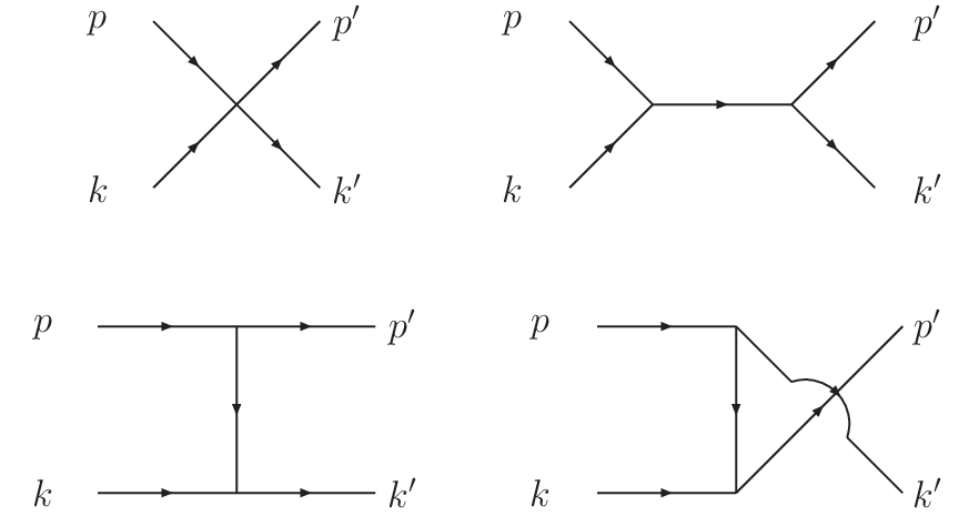
If the phonon dispersion relation is linear the , and -channel phonon exchange amplitudes diverge in the collinear limit. This corresponds to sub-sequent collinear splitting and joining processes with an on-shell propagator in between. The collinear processes should not contribute to the shear viscosity, but the numerical evaluation of collision integrals is more stable if the infrared divergence due to the on-shell propagator is regularized by including the thermal damping of the phonon propagator. For this purpose we compute the imaginary part of the self-energy correction to the phonon propagator.

There are two self-energy diagrams at , Fig. 3. The tadpole graph does not generate an imaginary part and we only compute the first diagram. We find
| (23) | ||||
The four-vector products are defined as , . This can be computed following Manuel:2004iv and we find
| (24) | ||||
The imaginary part of arises from the pole terms in the propagator. Analytic expressions for can be found in Appendix A. For very time-like external momenta
| (25) | ||||
and for space-like external momenta with
| (26) |
For the calculation these limiting forms provide sufficiently accurate representations of the exact one-loop expression in Eq. (24). We define the dressed phonon propagator
| (27) |
We can now collect the regularized , and -channel phonon exchange amplitudes. The -channel amplitude is
| (28) | ||||
The and -channel amplitudes follow from crossing symmetry. and . We have
| (29) | ||||
IV Variational Calculation
We are now in a position to compute the viscosity due to binary collisions. We have to solve the linearized Boltzmann equation Eq. (15) with the scattering amplitude determined in the previous section, and then compute the viscosity using either Eq. (7) or Eq. (16). This task is simplified by a number of useful properties of the linearized collision operator . The collision operator is a linear operator on the space of functions . With a suitably defined inner product this operator is hermitian and negative semi-definite. As a consequence it is possible to compute transport properties using eigenfunction and variational methods Resibois.
We elect to use the trial functions
| (30) |
where is a parameter that we choose for best convergence Chen:2006ig. The orthogonal polynomials of order are defined such that the coefficient of the highest power is 1 and that the orthogonality conditions Dobado:2001jf
| (31) |
are satisfied. Starting from we can recursively determine all the . This also defines the normalization factors . The polynomials are a generalization of the Sonine (modified Legendre) polynomials to Bose-Einstein statistics and linear dispersion relations.
Inserting the trial function into Eq. (7) we find the following expression for the viscosity
| (32) | ||||
Alternatively, we can use the trial function in Eq. (16). We get
| (33) |
where are the matrix elements of the linearized collision operator
| (34) | ||||
with the four-particle phase space factor
| (35) | ||||
Eqs. (32) and (33) are consistent provided
| (36) |
This is a simple linear equation for which is solved by
Once is determined we can extract the viscosity from Eq. (32). In practice we pick a value for and study convergence as the number of orthogonal polynomials is increased. What is nice about the method is that this is a variational procedure. One can show that Resibois
| (45) |
for any and sets of . The condition that the bound is optimized with respect to the expansion coefficients is equivalent to the consistency condition Eq. (36).
The scaling behavior of the viscosity with respect to the temperature and the Bertsch parameter is easily derived. We scale all momenta as . Using this fixes the scaling of the energies. All terms in the scattering amplitude have the same scaling behavior, except for a sub-leading correction due to the self-energy insertion in the phonon propagator. In terms of scaled momenta the phonon propagator can be written as
| (46) |
The scaling of the scattering cross section is , and the self energy term induces corrections that are functions of . We find
| (47) | ||||
where we have dropped the corrections due to the phonon self-energy. At the leading order in the polynomial expansion :
| (48) |
where we used . An interesting dimensionless quantity to consider is the ratio of viscosity to the entropy density for comparison with the conjectured bound discussed in the introduction, Eq. (2). The phonon gas entropy is
| (49) |
from which we obtain
| (50) |
In the calculation of in Eq. (33) the phase space integral can be reduced to a 5-dimensional integral. Of the original 12-dimensional integration variables four integrations are removed using the energy-momentum conserving delta function . We choose to constrain the three-momentum and the magnitude . Three more integrations can be removed as follows: without loss of generality we define the three-momentum along the -axis eliminating two angular integrations. Now, among the angular integration variables only the -axis projection of the three-momenta () and (), and the angular separation between and () are relevant. Thus the five remaining integration variables are: two magnitudes and , two angles and , and the angular difference . The 5-dimensional integration is done using the Monte Carlo routine Vegas Lepage:1980dq.

In addition to varying the parameter in the trial function , we check for convergence as we increase the number of terms inside the summation. From numerical experiments with integer , we find the maximal, convergent results for . In Fig. 4, we show at with for . Convergence as the order of the polynomial used in the trial function is varied is demonstrated. The solution at leading order of the polynomial expansion starts small, and then converges to the result. This is expected since the trial function at second order of the polynomial contains the trial function with .
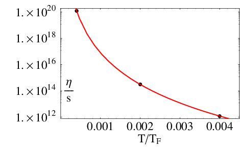
Fig. 5 shows at three temperatures for the best trial function with . The data is very well described by the functional form
| (51) |
which is also shown in the figure. The numerical results in Fig. 5 are stable to about . A comparison with the conjectured viscosity bound is shown in Fig. 6. The bound is violated for , which is close to the measured critical temperature TC for superfluidity where the phonon calculation is not reliable. In the region where the phonon calculation is reliable, the viscosity bound is satisfied.
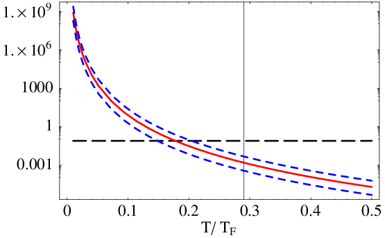
In Fig. 7 we compare our results to calculations in the high temperature limit and to experimental data. The high temperature results are taken from Bruun. These authors computed the viscosity due to binary fermion collisions. The free space cross section is proportional to . In the high temperature limit the infrared divergence is effectively cut off by the thermal momentum . For Bruun
| (52) |
In this limit the entropy density is that of a classical gas
| (53) |
The data points are based on a hydrodynamic analysis Schafer:2007pr of experimental data on the damping of collective excitations in a unitarity Fermi gas Kinast:2005.
We observe that the naïve extrapolation of the high and the low curves cross at around , which is indeed close to the transition temperature . This crude extrapolation of the two limiting curves for suggests that the viscosity minimum is about a factor 5 above the viscosity bound. This is quite consistent with the experimental data. We also note that the experimental data show the expected increase in for , but they do not show the rise for . This may be related to the fact that the phonon mean free path becomes so large that it is comparable to the size of the experimental Fermi gas sample and hydrodynamics does not apply.

V Conclusions
We computed the shear viscosity of a cold unitarity gas in the superfluid phase. For the viscosity is dominated by phonons, and the leading order effective Lagrangian for the phonons is characterized by a single universal parameter . This parameter can be extracted from the ground state energy of the unitarity gas.
The calculation is based on the linearized Boltzmann equation, and only the leading order phonon scattering processes are included. The shear viscosity is determined using a variational procedure. We find that the shear viscosity scales as . This result can be combined with high temperature calculations of the shear viscosity to provide an estimate of the location and magnitude of the viscosity minimum. We find that the minimum value of occurs close to , and that the value of is likely to exceed the proposed viscosity bound. A similar viscosity minimum is expected to occur in QCD. At low temperature the viscosity is dominated by weakly interacting Nambu-Goldstone bosons (pions and kaons) Prakash:1993bt; Dobado:2001jf; Chen:2006ig, and at high temperature the viscosity is governed by weakly interacting quarks and gluons Arnold:2003zc.
There are a number of issues that deserve further study. The viscosity of the superfluid unitarity gas has the same behavior as the viscosity of liquid Helium at low temperature. In the case of liquid Helium the viscosity is believed to be dominated by processes. On-shell phonon splitting processes can only occur if higher order corrections to the effective Lagrangian lead to a concave phonon dispersion relation [) with ]. For the unitarity Fermi gas we do not know whether this is the case. It is known that the Bogoliubov spectrum of a weakly interacting Bose gas has , so the role of these processes can be studied in an expansion around the Bose-Einstein limit.
In general we would like to extend the calculation to higher temperatures. In the vicinity of the we expect both bosonic and fermionic excitations to play a role. A possible starting point in this regime is provided by the expansion around spatial dimensions proposed in Nussinov:2004; Nishida:2006br. It is also interesting to improve the high temperature calculations by including correlations between the fermions. Some steps in this direction were taken in Bruun.
Acknowledgements.
The authors acknowledge helpful discussions with Dean Lee. This work was supported in parts by the US Department of Energy grant DE-FG02-03ER41260.Appendix A Analytic form for the self-energy
The imaginary part of arises from the pole terms in Eq. (24). We find (see Manuel:2004iv)
| (54) |
with
| (55) |
There are four terms, corresponding to . Terms with contribute for space-like momenta , and terms with contribute for time-like momenta. For space-like momenta we get
| (56) | ||||
The result for time-like momenta and is
| (57) | ||||
and . These integrals can be computed analytically in the limit of small momenta. In the space-like region we have . This implies and
| (58) |
For time-like momenta , and
| (59) | ||||
References
- (1) P. Danielewicz and M. Gyulassy, Phys. Rev. D31, 53 (1985).
- (2) G. Policastro, D. T. Son and A. O. Starinets, Phys. Rev. Lett. 87, 081601 (2001), [hep-th/0104066].
- (3) P. Kovtun, D. T. Son and A. O. Starinets, Phys. Rev. Lett. 94, 111601 (2005), [hep-th/0405231].
- (4) D. Teaney, Phys. Rev. C68, 034913 (2003), [nucl-th/0301099].
- (5) T. Hirano and M. Gyulassy, Nucl. Phys. A769, 71 (2006), [nucl-th/0506049].
- (6) T. D. Cohen, hep-th/0702136.
- (7) A. Dobado and F. J. Llanes-Estrada, hep-th/0703132.
- (8) K. M. O’Hara, S. L. Hemmer, M. E. Gehm, S. R. Granade and J. E. Thomas, Science 298, 2179 (2002); M. E. Gehm, S. L. Hemmer, S. R. Granade, K. M. O’Hara and J. E. Thomas, Phys. Rev. A 68, 011401(R) (2003).
- (9) T. Bourdel, J. Cubizolles, L. Khaykovich, K. M. F. Magalhães, S. J. J. M. F. Kokkelmans, G. V. Shlyapnikov and C. Salomon, Phys. Rev. Lett. 91, 020402 (2003).
- (10) K. Dieckmann, C. A. Stan, S. Gupta, Z. Hadzibabic, C. H. Schunck and W. Ketterle, Phys. Rev. Lett. 89, 203201 (2002).
- (11) C. A. Regal, C. Ticknor, J. L. Bohn and D. S. Jin, Nature 424, 47 (2003); M. Greiner, C. A. Regal and D. S. Jin, Nature 426, 537 (2003).
- (12) S. Jochim, M. Bartenstein, A. Altmeyer, G. Hendl, S. Riedl, C. Chin, J. Hecker Denschlag, and R. Grimm, Science 302, 2101 (2003).
- (13) P. Massignan, G. M. Brunn and H. Smith, Phys. Rev. A 71, 033607 (2005); G. M. Bruun and H. Smith, Phys. Rev. A 72, 043605 (2005), Phys. Rev. A 75, 043612 (2007).
- (14) I. M. Khalatnikov, An Introduction to the Theory of Superfluidity (W. A. Benjamin, Inc., 1965).
- (15) H. J. Maris, Phys Rev A, 1980 (1973).
- (16) C. Manuel, A. Dobado and F. J. Llanes-Estrada, JHEP 09, 076 (2005), [hep-ph/0406058].
- (17) E. M. Lifshitz and L. P. Pitaevskii, Physical Kinetics (Elsevier, 1987).
- (18) M. Greiter, F. Wilczek and E. Witten, Mod. Phys. Lett. B3, 903 (1989).
- (19) D. T. Son and M. Wingate, Annals Phys. 321, 197 (2006), [cond-mat/0509786].
- (20) D. T. Son, hep-ph/0204199.
- (21) J. Carlson, S.-Y. Chang, V. R. Pandharipande and K. E. Schmidt, Phys. Rev. Lett. 91, 050401 (2003).
- (22) S. Y. Chang, V. R. Pandharipande, J. Carlson and K. E. Schmidt, Phys. Rev. A 70, 043602 (2004).
- (23) G. E. Astrakharchik, J. Boronat, J. Casulleras and S. Giorgini, Phys. Rev. Lett. 93, 200404 (2004).
- (24) J. W. Chen and D. B. Kaplan, Phys. Rev. Lett. 92, 257002 (2004).
- (25) D. Lee, Phys. Rev. B73, 115112 (2006).
- (26) A. Bulgac, J. E. Drut and P. Magierski, cond-mat/0505374.
- (27) E. Burovski, N. Prokof’ev, B. Svistunov and M. Troyer, Phys. Rev. Lett. 96, 160402 (2006).
- (28) L. Luo, B. Clancy, J. Joseph, J. Kinast and J. E. Thomas, Phys. Rev. Lett. 98, 080402 (2007), [cond-mat/0611566].
- (29) P. Résibois and M. d. Leener, Classical Kinetic Theory of Fluids (John Wiley Sons, 1977).
- (30) J.-W. Chen and E. Nakano, Phys. Lett. B647, 371 (2007), [hep-ph/0604138].
- (31) A. Dobado and S. N. Santalla, Phys. Rev. D65, 096011 (2002), [hep-ph/0112299].
- (32) G. P. Lepage, CLNS-80/447.
- (33) T. Schafer, cond-mat/0701251.
- (34) J. Kinast, T. A. and T. J. E., Phys. Rev. Lett. 94, 170404 (2005), [cond-mat/0502507].
- (35) M. Prakash, M. Prakash, R. Venugopalan and G. Welke, Phys. Rept. 227, 321 (1993).
- (36) P. Arnold, G. D. Moore and L. G. Yaffe, JHEP 05, 051 (2003), [hep-ph/0302165].
- (37) Z. Nussinov and S. Nussinov, cond-mat/0410597.
- (38) Y. Nishida and D. T. Son, Phys. Rev. Lett. 97, 050403 (2006), [cond-mat/0604500].