Increasing future gravitational-wave detectors sensitivity by means of amplitude filter cavities and quantum entanglement

Following the article Corbitt2004-3, consider a resonance-tuned filter cavity pumped through its input mirror IM by squeezed vacuum (see Fig. 1). Suppose that the cavity end mirror EM is also partly transparent, and the following condition is satisfied for the mirrors power transmittance and the cavity losses per bounce:

The cavity tuned in such a way is transparent at low sideband frequencies $\Omega\ll\gamma_{f}$ and have reflectivity close to unity at high frequencies $\Omega\gg\gamma_{f}$. Therefore, the reflected beam which is fed into the gravitational wave detector dark port will be squeezed only at high frequencies. At low frequencies the squeezed state will be replaced by the vacuum state created partly by the end mirror transmittance and partly by the cavity optical losses.

It has to be noted that it was supposed in the article Corbitt2004-3 that only one (input) mirror of the filter cavity is partly transparent: $T_{E}=0$ and $T_{I}=A_{f}$. However, using modern high-reflective mirrors, it is possible to obtain $A_{f}\ll T_{I}$ and, therefore, $T_{E}\approx T_{I}$. Really, the filter cavity half-bandwidth has to be close to $\gamma_{f}\sim 2\pi\times 100\,{\rm s}^{-1}$. Therefore, there has to be $T_{I}^{2}=2l_{f}\gamma_{f}/c\sim 10^{-4}$. Taking into account that, with the best mirrors available now, the filter cavity losses per bounce can be as small as $A_{f}^{2}\approx 10^{-5}$, it is possible to provide the value of $1-\eta_{f}=1-T_{E}^{2}/T_{I}^{2}=A_{f}^{2}/T_{I}^{2}\sim 0.1$ .

It is shown in Appendix A, that squeezing factors for the phase and amplitude quadrature components of the filter cavity output beam are equal to

and these noises are non-correlated:

It is easy to see, that

It follows from Eqs. (3, 4), that there is a redundant quantum noise in the filter cavity output beam which is maximal at $\Omega=\gamma_{f}$ and vanishes if $\Omega\to 0$ or $\Omega\to\infty$, i.e., if the filter cavity is completely reflective or completely transparent.

Consider the beam which leaves the filter cavity through the end mirror EM. It is squeezed at low frequencies $\Omega<\gamma_{f}$. Squeezing factors of the corresponding phase and amplitude quadrature components are equal to (see Appendix A)

and these quadratures are also non-correlated, $S_{\varphi A,{\sf E}}(\Omega)=0$.

Redundant noise exists at this output too:

At the same time, there is cross-correlation between the corresponding (phase and amplitude) quadrature components at the filter cavity two outputs:

Equations (4, 6, 7) reflect a well-known feature of entangled bipartite quantum systems. Even if the whole system is in a pure quantum state, each of the parties detected individually appear as being in a mixed state. In the particular case of the optical fields at the filter cavity two outputs, this leads to the inequalities (4, 6). At the same time, measurement of each of the parties project the another one into a pure state, utilizing the mutual information [in our case, the cross-correlation (7)] which exists in the system due to the entanglement.

In the particular case considered here, measurement of the optical field leaving the filter cavity though the end mirror, allows to reduce effective fluctuations of the optical field reflected from the filter cavity input mirror, compare Eqs. (12) and (15) below.

The component of output signal of the main homodyne detector (MHD in Fig. 1) created by the optical quantum noise is proportional to

where $x_{\rm fl}(\Omega)$ is is the measurement noise and $\hat{F}_{\rm fl}(\Omega)$ is the back-action force, see Eqs. (50, 51). Spectral density of the noise (8) is equal to:

where

are spectral densities of the noises $\hat{x}_{\rm fl}(\Omega)$ and $\hat{F}_{\rm fl}(\Omega)$, correspondingly, see Appendix B. The second term in the square brackets in Eq. (10a) arises due to the homodyne detector non-unity quantum efficiency $\eta<1$.

Due to Heisenberg’s uncertainty relation, spectral densities (10) satisfy the following inequality 92BookBrKh; 03a1BrGoKhMaThVy:

where $S_{xF}$ is cross-correlation spectral density, which is equal to zero in this particular case. Without optical losses or other non-fundamental noise sources, there has to be exact equality in this formula. However, it follows from Eq. (4) that even in the case of $\eta=1$, product of spectral densities (10) is equal to

Therefore, this meter is not optimal from the quantum measurements theory point of view. The origin of this fact is, evidently, the information loss in the filter cavity. Part of this loss created by the light absorption on the filter cavity is inevitable. But the other part created by the information leak through the filter cavity end mirror can be eliminated using the correlation (7).

Really, suppose that some quadrature component $\hat{\rm q}_{\zeta}$ of the end mirror output beam, defined by the homodyne angle $\zeta$ [see Eq. (52)], is monitored using the additional homodyne detector AHD. Due to the correlation (7), this detector provides some information about the quantum fluctuations (8). Therefore, mixing in optimal way the main detector output with the additional detector output, it is possible to reduce the sum quantum noise. It is shown in Appendix C, that this optimized sum noise spectral density is equal to

where

are spectral densities of the effective measurement noise, effective back action force and the corresponding cross spectral density [for the explicit expressions, see Eqs. (60)], $S_{\zeta}(\Omega)$ is the spectral density of the additional detector output [see Eq. (53)], and $S_{x\zeta}(\Omega)$, $S_{F\zeta}(\Omega)$ are the corresponding cross spectral densities [see Eqs. (55)]. It can be shown, that if $\eta=1$, then the spectral densities (14) satisfy the following uncertainty relation:

where $S_{\zeta}(\Omega)$ is the noise ${\rm q}_{\zeta}$ spectral density [compare with Eq. (12)]. In the ideal no-losses case of $\eta_{f}=1$, the RHS of this equation is equal to $\hbar^{2}/4$, which means that the noises in this case are as small as allowed by quantum mechanics.

Spectral density (13) depends on two free parameters: $\zeta$ and $\gamma_{f}$, which should be tuned in some optimal way. It is evident that there is no the unique universal optimization here, and the choice of $\zeta$ and $\gamma_{f}$ depends on the desired shape of $S_{\rm sum}^{\rm eff}(\Omega)$. Below we will use the following simple procedure which provides smooth broadband spectral density.

Consider the ratio of $S_{\rm sum}^{\rm eff}(\Omega)$ to the spectral density of the corresponding ordinary (without squeezing) meter with increased by $e^{r}$ optical power:

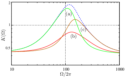
“Corresponding” means that the both meters has the same values of $m$ and $\gamma$. Characteristic spectral dependences of $K(\Omega)$ is shown in Fig. 2. There is one maximum here close to the frequency $\Omega=\gamma_{f}$, and if $\Omega\ll\gamma_{f}$ or $\Omega\gg\gamma_{f}$, then $K(\Omega)\approx e^{-r}$. We will use the values of $\zeta$ and $\gamma_{f}$, which provide the minimal value of this maximum.

In this subsection, we suppose that the interferometer half-bandwidth $\gamma$ is equal to $\gamma_{0}$. Below this case will be referred to as “conventional interferometer”.

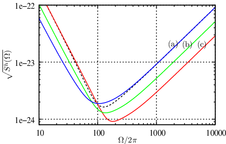
In Fig. 3, we plot the quantum noise spectral densities of the scheme with the additional detector considered above, of the original CMW scheme and of the SQL-limited (unsqueezed) interferometer. The noises are normalized as equivalent strain fluctuations:

The circulating optical power $W$ is supposed to be equal to the value planned for the Advanced LIGO ($W_{0}=840\,{\rm kW}$). It is easy to see that the additional detector allows to significantly reduce the noise at medium and low frequencies, compare lines (a) and (b). At low frequencies, the noise virtually does not differ from the one of the ordinary interferometer (without filter cavity).

It is well known that reducing the optical power, it is possible to increase sensitivity at low frequencies (in the radiation-pressure noise domination area), sacrifying the high-frequency sensitivity (in the shot noise domination area). In Fig. 4, the noises of the scheme considered here are plotted for the following three values of the optical power: $W_{0}\,e^{-2r}=84\,{\rm kW}$, $W_{0}\,e^{-r}=266\,{\rm kW}$, and $W_{0}=840\,{\rm kW}$, together with the quantum noise of the conventional unsqueezed interferometer at $W=840\,{\rm kW}$.

The power $W=W_{0}\,e^{-r}$ provides almost even gain in the quantum noise spectral density in the all frequency band [see line (b)], similar to the regime with frequency-dependent homodyne angle Unruh1982; 02a1KiLeMaThVy. The gain value is smaller than in the latter case, $e^{r}$ vs.​ $e^{2r}$. However, the required optical power is also $e^{r}$ times smaller. Regime with $W=W_{0}\,e^{-2r}$ allows to reduce the quantum noise spectral density at low frequencies by $e^{2r}$, while keeping the high-frequency noise at the same level as in the unsqueezed interferometer.

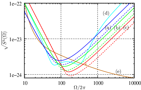
In Fig. 5, we plot the quantum noise spectral densities for the same parameters values as in Fig. 4, but taking into account non-unity quantum efficiency $\eta$ of the photodetectors (solid lines). It is easy to observe significant sensitivity degradation at high frequencies (where the light is squeezed). At the same time, the sensitivity virtually is not affected at low frequencies. For comparison, spectral densities of the sum quantum noise $S^{h}_{\rm quant}$ and the sum technical noise $S^{h}_{\rm tech}$ planned for the Advanced LIGO and calculated using the bench program benchsite are also plotted in Fig. 5.

In Table 2, numerical estimates of the sensitivity are presented. Two criteria are used in this Table. The first one is the signal to noise ratio for neutron star - neutron star (NSNS) inspiral waveforms Buonanno2004, normalized by the value corresponding to the conventional (unsqueezed) interferometer with $\gamma=\gamma_{0}$ and $W=W_{0}$:

Here $f_{c}=10\,\mathrm{Hz}$ is the gravitational-wave detector low-frequency cut-off, and $f_{\mathrm{ISCO}}=1570\,\mathrm{Hz}$ is the gravitational-wave frequency corresponding to the Innermost Stable Circular Orbit of a Schwarzchild black hole with mass equal to $2\times 1.4$ solar masses. This criterion characterizes the low-frequency sensitivity. The second criterion is the sensitivity for high-frequency periodic sources, which is simply the reciprocal value of the noise spectral density at some given frequency. Similar to Corbitt2004-3, we use frequencies $f=1\,{\rm kHz}$ and $f=10\,{\rm kHz}$, and normalize the noise by the value corresponding to the conventional unsqueezed interferometer with $\gamma=\gamma_{0}$ and $W=W_{0}$:

The choice of $\gamma=\gamma_{0}$, while convenient for comparison with the simplest unsqueezed SQL-limited case, does not provide the best results. Increasing not just the optical power but also the interferometer bandwidth, it is possible to improve the sensitivity at high frequencies without sacrifying the low-frequency sensitivity. Really, it follows from Eqs. (9,13), that the low- and-high frequency asymptotics of the quantum noise spectral density are equal to

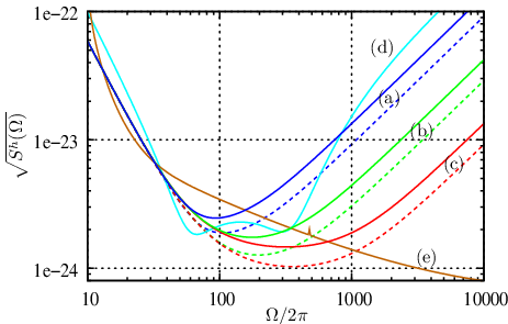
Therefore, if $\gamma$ increases proportionally to $J\propto W$, then the low-frequency asymptotic of $S^{x}(\Omega)$ remains unchanged, and the high-frequency one decreases proportionally to $J^{2}\propto W^{2}$. This consideration is illustrated by Fig. 6, where the quantum noise spectral density is plotted for the same values of the optical power as in Fig. 5, but for proportionally increased values of $\gamma$. The corresponding numerical estimates are also shown in Table 2 (see the last two rows).

References

- (1) Thomas Corbitt, Nergis Mavalvala, and Stan Whitcomb, Physical Review D 70, 022002 (2004).
- (2) A.Abramovici et al, Science 256, 325 (1992).
- (3) Ando M. et al., Physical Review Letters 86, 3950 (2001).
- (4) B.Willke et al., Classical and Quantum Gravity 19, 1377 (2002).
- (5) http://www.ligo.caltech.edu.
- (6) http://geo600.aei.mpg.de.
- (7) http://tamago.mtk.nao.ac.jp.
- (8) K.S.Thorne, The scientific case for mature ligo interferometers, 2000, LIGO document P000024-00-R (www.ligo.caltech.edu/docs/P/P000024-00.pdf).
- (9) P.Fritschel, Second generation instruments for the Laser Interferometer Gravitational-wave Observatory (LIGO), in Gravitational Wave Detection, Proc. SPIE, volume 4856-39, page 282, 2002.
- (10) http://www.ligo.caltech.edu/advLIGO.
- (11) http://www.icrr.u-tokyo.ac.jp/gr/LCGT.html.
- (12) K.McKenzie, N.Grosse, W.P.Bowen, S.E.Whitcomb, M.B.Gray, D.E.McClelland, P.K.Lam, Physical Review Letters 93, 161105 (2004).
- (13) H.Vahlbruch, S.Chelkowski, B.Hage, A.Franzen, K.Danzmann, and R.Schnabel, Physical Review Letters 97, 011101 (2006).
- (14) C.M.Caves, Physical Review D 23, 1693 (1981).
- (15) W.G.Unruh, in Quantum Optics, Experimental Gravitation, and Measurement Theory, edited by P.Meystre and M.O.Scully, page 647, Plenum Press, New York, 1982.
- (16) H.J.Kimble, Yu.Levin, A.B.Matsko, K.S.Thorne and S.P.Vyatchanin, Physical Review D 65, 022002 (2001).
- (17) Jan Harms, Yanbei Chen, Simon Chelkowski, Alexander Franzen, Hennig Vahlbruch, Karsten Danzmann, and Roman Schnabel, Physical Review D 68, 042001 (2003).
- (18) A.Buonanno, Y.Chen, Physical Review D 69, 102004 (2004).
- (19) A.Buonanno, Y.Chen, Physical Review D 64, 042006 (2001).
- (20) A.Buonanno, Y.Chen, Physical Review D 65, 042001 (2002).
- (21) V.B.Braginsky, F.Ya.Khalili, Quantum Measurement, Cambridge University Press, 1992.
- (22) V.B.Braginsky, M.L.Gorodetsky, F.Ya.Khalili, A.B.Matsko, K.S.Thorne and S.P.Vyatchanin, Physical Review D 67, 082001 (2003).
- (23) http://ilog.ligo-wa.caltech.edu:7285/advligo/Bench.
- (24) A.Buonanno, Y.Chen, Physical Review D 67, 062002 (2003).
- (25) F.Ya.Khalili, Physical Review D 75, 082003 (2007).