Grain boundary energies and cohesive strength as a function of geometry
Abstract
Cohesive laws are stress-strain curves used in finite element calculations to describe the debonding of interfaces such as grain boundaries. It would be convenient to describe grain boundary cohesive laws as a function of the parameters needed to describe the grain boundary geometry; two parameters in 2D and 5 parameters in 3D. However, we find that the cohesive law is not a smooth function of these parameters. In fact, it is discontinuous at geometries for which the two grains have repeat distances that are rational with respect to one another. Using atomistic simulations, we extract grain boundary energies and cohesive laws of grain boundary fracture in 2D with a Lennard-Jones potential for all possible geometries which can be simulated within periodic boundary conditions with a maximum box size. We introduce a model where grain boundaries are represented as high symmetry boundaries decorated by extra dislocations. Using it, we develop a functional form for the symmetric grain boundary energies, which have cusps at all high symmetry angles. We also find the asymptotic form of the fracture toughness near the discontinuities at high symmetry grain boundaries using our dislocation decoration model.
pacs
62.20.Mk, 61.72.Mm, 31.15.QgI Introduction
In materials such as silicon and various aluminum alloys, cracks initiate and propagate along the interfaces between polycrystals known as grain boundaries. When the cracks initiate at the site of these microscopic defects, the macroscopic fracture strength of the material is dependent on the microscopic structure of the grain boundaries. The debonding of an interface such as a grain boundary is described by a cohesive law, giving the displacement across the interface as a function of stress (figure 1).
Cohesive laws are used by finite element cohesive zone models, which simulate fracture initiation at interfaces Needleman 1990. It has been shown that the shape and scale of the cohesive law has a large effect on the outcome of the finite element simulation Needleman 1990; Falk et al. 2001. However, the CZM studies of grain boundary fracture have used cohesive laws that are guessed, chosen for numerical convergence, and do not take into consideration the effect of varying grain boundary geometries within the material – the same cohesive law is often used throughout the material despite the fact that in a real material, grain boundaries of varying geometries must occur Iesulauro et al. 2002; Iesulauro et al. 2003; Warner et al. 2006.
It would be useful to find a formula for the cohesive laws of the grain boundaries of a given material as a function of geometry, for input into finite element simulations. The geometry of a 3D grain boundary depends on 5 parameters that describe the orientations of the two grains. In addition, there are three different modes of fracture (normal to the crack plane, shear in a direction parallel to the crack line, or shear in a direction perpendicular to the crack line) to explore 11 1 For cracks propagating through a grain boundary, the direction of the crack front in relation to the structure of the grain boundary may affect the fracture toughness, but this dependence is not included in cohesive laws. as well as dependencies on temperature, impurities at the interface, and emission of dislocations to consider.
Thus far, no systematic study of grain boundary cohesive laws as a function of geometry has been done with molecular dynamics or experiment. There is difficulty in measuring cohesive laws experimentally because it is difficult to isolate and measure the displacements on either side of the grain boundary.

Previous atomistic studies of the mechanical response of grain boundaries have concentrated on a small number of symmetric grain boundaries in 3D Chen et al. 1989; Sansoz and Molinari 2004; Sansoz and Molinari 2005; Shenderova et al. 2000; Spearot et al. 2004; Warner et al. 2006. Exploring the complete picture of 3D grain boundary cohesive laws involves exploring a 5-dimensional space with three modes of fracture. Because of this difficulty, we have taken a step back. We seek to systematically explore the cohesive laws for mode I fracture for all possible grain boundary geometries in 2D that can be simulated in periodic boundary conditions for a particular size and strain. We will initially be focusing on symmetric grain boundaries and then expanding the picture to look at asymmetric 2D grain boundaries. One use of such data would be for finite element simulations of polycrystals Coffman et al. 2007, as described above. For this purpose, it would be nice to find a functional form which describes the fracture strength of the grain boundary as a function of geometry.
We find, however, that the fracture strength as a function of tilt angles is discontinuous everywhere, with particularly large jumps at special, high symmetry grain boundaries composed of a simple arrangement of structural units with a low repeat distance. These special boundaries are also associated with cusps in the grain boundary energy. We will describe dependence of the energy and the fracture strength near these special boundaries by treating them as perfect, albeit complex, crystals with added dislocations to break the symmetry.
Most studies use the coincidence site model Bollmann 1970 to construct and classify special grain boundaries Chen et al. 1989; Sansoz and Molinari 2004; Sansoz and Molinari 2005; Shenderova et al. 2000; Warner et al. 2006 while a few mention the significance of structural units Bishop and Chalmers 1968; Chen et al. 1989; Ishida 1976; Sansoz and Molinari 2005; Wolf and Merkle 1992. The only 2D study we are aware of, the “bubble-raft” model, observes the structural units of several of the special, high angle grain boundaries for the triangular lattice and how patterns of structural units combine to create vicinal geometries Ishida 1976. Other 3D studies discuss how grain boundaries with geometries close to those of special grain boundaries can be decomposed into the structural unit of the special grain boundary with added flaws Bishop and Chalmers 1968; Wolf and Merkle 1992. We develop a systematic way of finding high symmetry geometries and show that the combinations of patterns of structural units at vicinal grain boundaries are key to understanding the dependence of energy and fracture strength on geometry.
Sansoz and Molinari find the grain boundary energy by allowing the grains to relax together from an initial separation of a few angstroms Sansoz and Molinari 2005 while others perform a conjugate gradients search Chen et al. 1989. We use a systematic method for explicitly imposing a relative shift between the grain and using atomistic relaxation for finding the global energy minimum similar to that used in Sansoz and Molinari 2004; Wolf and Merkle 1992. It is well established that there exist cusps in the grain boundary energy for special high angle grain boundaries Chen et al. 1989; Harrison et al. 1976; Pumphrey 1976; Sansoz and Molinari 2005; Shenderova et al. 2000; Wolf 1992; Wolf and Merkle 1992; Wolf and Jaszczak 1992. Recent studies of grain boundary constitutive properties focus on the response to shear Sansoz and Molinari 2005; Warner et al. 2006 or compare shear and tension Sansoz and Molinari 2004; Spearot et al. 2004. Warner et al. claim that the tensile response does not depend on the geometry of the grain boundary Warner et al. 2006. Others have seen jumps in the tensile fracture strength at high angle grain boundaries geometries Chen et al. 1989; Shenderova et al. 2000.
We will explain the cusps in energy and jumps in fracture strength by drawing an analogy between perfect crystals and high symmetry, high angle grain boundaries. The dislocation model of low angle grain boundaries gives a form for the grain boundary energy. Because vicinal grain boundaries can be thought of as high symmetry grain boundaries with added flaws, the energy cusps at special grain boundaries have the same form. A similar argument will apply to the peak fracture stress. Just as adding dislocations to the perfect crystal adds a nucleation point for fracture, and therefore a discontinuity (jump down) in fracture strength, adding a flaw to a high symmetry, high angle grain boundary abruptly changes the local fracture strength by adding a potential nucleation site for fracture.
II Procedure for Calculating Grain Boundary Energy and Cohesive Strength
We calculate energies and cohesive strengths for grain boundaries using the DigitalMaterialBailey et al. 2006 package to perform atomistic simulations. The potential we are using for 2D simulations is the Lennard Jones potential with a smooth, fourth order cutoff between 2.41 and 2.7 Å. The ground state is a triangular lattice with a lattice constant of 1.11 Å.
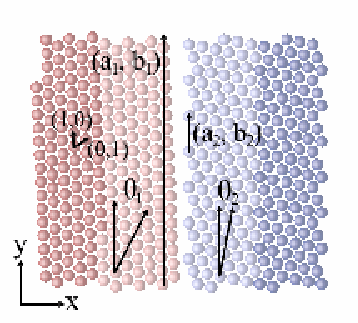
We set up the grain boundary by initializing two rectangular grains with the given rotations that define the grain boundary geometry we wish to measure. An example of the configuration of atoms that make up a grain boundary simulation is shown in figure 2. We use periodic boundary conditions in the -direction in order to avoid edge effects which could potentially cause cracks to nucleate at the intersection with the surface 22 2 Another alternative is to use a layer of constrained atoms. Typically, in a finite element simulation of a subsection of a material, the nodes on the surfaces of the model are constrained to not move in a direction perpendicular to the surface. This is known as “rollered” boundary conditions. We can imitate these boundary conditions in an atomistic simulation by constraining a layer of atoms at the surface or edge of the simulation to not move perpendicular to that surface or edge. This will partially ameiliorate the edge effects, suppress the Poisson effect, and has the advantage of allowing us to simulate grain boundaries of any geometry Coffman et al. 2007. We have compared simulations of different sizes with rollered boundary conditions in the -direction to a simulation of the same geometry, but with periodic boundary conditions in the -direction. We see that if we use rollered boundary conditions, we need a simulation that is 48 times longer in the -direction in order to converge to within 2% of the results found by a simulation with periodic boundary conditions. Hence, for computational efficiency, we choose to use periodic boundary conditions in the -direction.. This has the disadvantage of only allowing geometries that have finite repeat distances. A method for finding these geometries is discussed in detail in section III.2. If necessary, both grains are strained slightly by equal and opposite amounts in order to have both grains fit into a periodic box. We use a constrained layer of atoms to impose fixed boundary conditions in the -direction. These are represented by the darker atoms in figure 2. The constrained layer of atoms has a width equal to twice the cutoff distance of the potential to eliminate surface effects from the free atoms.
Besides the tilt angles, there are other factors to consider in constructing the grain boundary geometries. For commensurate grain boundaries, there will be an ideal relative displacement in the direction parallel to the grain boundary (the -direction in figure 2). This ideal displacement will correspond to the lowest energy and thus is the most natural configuration for a given pair of tilt angles. 33 3 The Frenkel-Kontorova model Frenkel and T. 1938 describes a one dimensional chain of atoms, connected by springs, subject to an external, sinusoidal potential. If the relaxed length of the spring and the width of the potential wells are commensurate a minimum energy state exists. For the incommensurate case, there will be a pinned phase with many local minima and an unpinned phase, depending on the depth of the wells in relation to the stiffness of the springs.
We find the displacement along the boundary which gives the lowest energy by initializing the two grains with a small displacement in the -direction and varying displacements in the -direction, relaxing the atoms (with the boundary layers contrained to be rigid and non-rotating), and measuring the grain boundary energy per length. The range of displacements in the -direction that we must search over is given by
| (1) |
where we assume . This is illustrated in figure 3. The grain boundary energy per length is defined as
| (2) |
where is the total potential energy for the configuration of atoms (excluding the constrained atoms), is the number of unconstrained atoms, is the energy of a single atom in the bulk, and is the length of the grain boundary. An example of the results of such a search is shown in figure 4. The regions with the same final displacement and energy correspond to basins of attraction around the finite number of final configurations of atoms. The minimized energy per unit length (equation 2) found by this method is what we record as the grain boundary energy.


We have also tried thermal annealing and have found that for certain geometries, the grain boundary migrates to form a jagged interface with segments of different grain boundaries that collectively have a lower total energy than the geometry given by the original set of tilt angles. The tendency of certain grain boundaries to corrugate is also discussed by Ishida and Pumphrey Ishida 1976; Pumphrey 1976. As a corrugated grain boundary is torn apart to measure the cohesive law, the corners form stress concentrations which weaken the grain boundary. Despite the fact that this configuration may be more natural, it is not what we intend to measure. We wish to measure the fracture toughness of all possible pairs of tilt angles, even if those pairs of tilt angles happen to be unstable. In a few cases, the minimization procedure described above produced a curved grain boundary. In these cases, we constrained the displacements in the -direction such that a consistent pattern of flaws along a straight grain boundary is achieved.
After finding the ideal -displacement, we increment the strain by displacing the constrained layers of atoms in the -direction, away from the grain boundary. We relax the atoms and measure the force in the -direction per unit length on the constrained layer of atoms. If the measurement of the stress drops abruptly during one strain step, the simulation restores the positions from a previous step, reduces the size of the strain increment, and proceeds. The result of such a simulation is shown in figure 1. The maximum stress in the stress strain curve is what we define as the peak stress.
III Grain Boundary Geometries
III.1 Lattice Symmetries and Tilt Angles
For the triangular lattice, it is clear that we only need to explore tilt angles between 0∘ and 60∘, but we can further reduce the space of grain boundary geometries to consider. Figure 5 represents the space of tilt angle pairs. Reflecting a point in this space through the line corresponds to swapping the two grain orientations which, as shown in figure 5, is equivalent to flipping the grain boundary in both the vertical and horizontal directions, resulting in the same grain boundary. Reflecting through the point takes to , reversing the sense of rotation of each grain. As shown in figure 5, this is equivalent to flipping the grain boundary in the vertical direction. Reflecting through the line takes to , both switching the grains and reversing the senses of rotation. This is equivalent to flipping the grain boundary in the horizontal direction, also shown in figure 5. Thus, we only need to consider the pairs of tilt angles in the triangle enclosed by the line, the line, and the line – the shaded region in figure 5.

III.2 Finding All Possible Geometries for Periodic Boundary Conditions
In order to better simulate the grain boundary in the bulk as described in section II, we would like to use periodic boundary conditions along the direction of the grain boundary (-direction). In order to simulate 2D grain boundaries in periodic boundary conditions, we need not only for both grain orientations to have finite repeat distances, but also for the repeat distances to be commensurate with one another. Let be the lattice vector that is parallel to the edge of a 2D triangular lattice. Since the basis vectors are at a 60∘ angle to one another, the repeat distance of a particular orientation of a 2D triangular lattice is given by
| (3) |
The tilt angle is then given by
| (4) |
In order to expand the number of possible geometries, we have also considered geometries for which applying a small strain to each grain allows us to fit both grains inside the same periodic box. For any pair of orientations that have repeat distances that are not commensurate, we can find a continued fraction approximation to the ratios of their lengths, . We can strain each grain equally into a box of size , where the strain required is . For a strain of 0.05%, the grain boundary would have to be 1,000 Å long before the strain would alter the structure of the grain boundary. We find all pairs of tilt angles that correspond to commensurate or near commensurate grain boundaries by looping over pairs of surface vectors and comparing the repeat distances.

Figure 6 shows all possible geometries that can be simulated with a periodic length of 70 lattice constants or less, and a strain of 0.05% or less. The line corresponds to perfect crystals, while the line corresponds to symmetric grain boundaries. There is a gap near each of these lines because creating very small angle grain boundaries, or a geometry very close to symmetric grain boundaries, requires adding flaws that are separated by large distances. We see gaps near other high symmetry grain boundaries for the same reason. High symmetry grain boundaries are discussed in section III.3. The lines radiating out from high symmetry grain boundaries represent adding single flaws to those high symmetry grain boundaries at larger and larger distances, as you approach the high symmetry boundary. Each line represents a different type of flaw. The symmetry about the line is due to the fact that grains with tilt angles and have the same repeat distance. Therefore, the grain boundaries given by the tilt angles and have the same overall repeat distance, though these are different grain boundaries.
III.3 High Symmetry Grain Boundaries
Certain grain boundary geometries have particularly low repeat distances. These grain boundaries have special properties. They mark the center of cusps in the grain boundary energy and discontinuous increases in the fracture strength as a function of tilt angle. Table 1 show examples of high symmetry grain boundaries and figure 7 shows examples of geometries in between, which constitute adding a single flaw per supercell repeat distance to the high symmetry grain boundary. Note how the added flaws constitute a compromise between the two high symmetry geometries. Furthermore, a less high symmetry grain boundary can be repeated, and again have a single flaw added. Because of this hierarchical procedure for constructing lower-symmetry boundaries, the grain boundary energy and fracture strength as a function of tilt angle will have a self similar nature.
| Miller | Repeat Distance | Structure | ||
| Indices | (lattice constants) | |||
| 49.10 | (1,4) | 2.64 | 7 | ![[Uncaptioned image]](0707.1060v2/1-4.png) |
| 43.89 | (2,5) | 3.61 | 13 | ![[Uncaptioned image]](0707.1060v2/2-5.png) |
| 53.41 | (1,7) | 4.35 | 19 | ![[Uncaptioned image]](0707.1060v2/1-7.png) |
| 40.89 | (1,2) | 4.58 | 21 | ![[Uncaptioned image]](0707.1060v2/1-2.png) |
| 38.94 | (4,7) | 5.56 | 31 | ![[Uncaptioned image]](0707.1060v2/4-7.png) |
| 51.78 | (2,11) | 7.0 | 49 | ![[Uncaptioned image]](0707.1060v2/2-11.png) |
The coincidence site lattice model (CSL) describes grain boundaries in terms of , the inverse density of lattice sites that are shared by the two grain orientations when rotated about a common lattice point Bollmann 1970. In 2D, CSL grain boundaries are necessarily commensurate and vice versa. For the triangular lattice, each common lattice point for a given pair of grain orientations has a repeat cell that is an equilateral triangle with one edge defined by the surface vector with length . is equal to the number of lattice points inside this cell and is given by the area of the cell divided by the area of one lattice triangle, . While the CSL formulation gives a simple method for finding commensurate grain boundaries, it is misleading to suggest that the actual coincidence of sites plays a physical role. In fact, shifting the grains in the -direction so as to minimize the grain boundary energy (described in section II) generally causes the atoms to no longer coincide. Without this shift, the two free surfaces will have atomic planes that meet at the same point. The elastic energy is lowered by staggering the dislocations Hirth and Lothe 1982. Wolf has pointed out that for 3D, the CSL formulation of grain boundaries involves a redundant number of parameters Wolf 1992.
Bishop and Chalmers introduced the concept of “structural units” - polygonal structures of atoms along high angle grain boundaries Bishop and Chalmers 1968. We find that the patterns of “structural units” are more relevant to the physical properties of the grain boundaries. When relaxed, the structural units of grain boundaries in 2D, triangular lattices are 5 atoms forming a regular pentagon or a pentagon that is slightly stretched. Each high symmetry grain boundary is comprised of a simple pattern of pentagonal structural units (table 1). When a high symmetry grain boundary is perturbed, an element of the pattern of structural units from the neighboring high symmetry grain boundary is introduced (figure 7). As the tilt angles move closer to the neighboring high symmetry grain boundary, the flaws become closer together until they outnumber the original structure. The roles of flaw and original structure are then reversed. In this manner, combinations of patterns of structural units can be used to build up any commensurate, high angle grain boundary.

We find the structural units a useful way of conceptualizing the different grain boundary geometries. We have not found the coincidence site lattice model useful in our investigations. In systematically constructing grain boundaries with small repeat distances (section III.2), we have found the surface lattice vectors of the two sides of the grain boundary to be a useful description. We suggest that the structure of high angle grain boundaries can best be described in terms of a dislocation model. The “extra flaws” added to create vicinal grain boundaries can be described as partial dislocations. Figure 7 shows how to find the Burger’s vectors for the added flaws by examining the flaw in the pattern of structural units. 44 4 Since this Burger’s vector may be a sum of lattice vectors from either side of the grain boundary, the total may not be a full translation vector of the triangular lattice. We will show in section V.2 that this model gives excellent agreement in the stress field due to the added flaws, outside the background of the original flaw structure. We will show in sections IV and V that the dislocation model provides the most powerful framework for understanding the geometry dependence of the properties of grain boundaries.
IV Grain Boundary Energy
We have measured the grain boundary energy and peak stress for all symmetric grain boundaries with repeat distances under 20 lattice constants and asymmetric grain boundaries with repeat distances under 30 lattice constants. In order to explore the regions close to high symmetry grain boundaries, we have added a few geometries with longer repeat distances, close to the high symmetry grain boundaries.
The energy 55 5 We use ’energy’ for ’energy per unit length’ throughout. associated with the series of flaws that make up the grain boundary is defined in equation 2. As stated earlier, and found by several earlier studies Sansoz and Molinari 2005; Chen et al. 1989; Harrison et al. 1976; Pumphrey 1976; Wolf 1992; Palumbo and Aust 1992; Wolf and Jaszczak 1992, cusps appear at high symmetry boundaries. For small angle grain boundaries, the grain boundary energy has the form
| (5) |
where is the shear modulus, is the Burger’s vector, is the Poisson ratio, and is a factor that includes the core energy Hirth and Lothe 1982. One can now imagine the same scenario applied to high symmetry boundaries. We can take a high symmetry grain boundary and add or subtract flaws a distance apart as shown in figure 8. By the same reasoning as used for the low angle grain boundaries, the energy near the high symmetry grain boundary will have the form
| (6) |
where is the energy of the high symmetry grain boundary which occurs at the angle and incorporates the core energy of the flaw within the pattern of flaws.


The grain boundary energies for all of the symmetric grain boundaries that we have measured are shown in figure 9. Note that cusps occur at the angles listed in table 1. We are able to fit the data for symmetric grain boundaries to a function of the form
The first two terms fit the cusps at 0∘ and 30∘, where the cusps are symmetrical about their respective center points. The next set of terms in the sum fit the cusps at high symmetry tilt angles. The function was chosen as a fitting function because it asymptotically gives a shaped cusp in the near vicinity of and because it has the correct symmetry: even mirror symmetry at 0∘ and 30∘ and an overall period of 60∘. We use one term that is antisymmetric about and one term that is symmetric about so that we can fit the shape on either side of the cusp independently. We do not expect the slope of the curve on either side of the cusp to be the same since the Burger’s vectors of the additional flaws for the geometries on either side of the high symmetry geometry may differ (figure 7).
The can be any angles that have the shortest repeat distances, such as those given in table 1. The curve in figure 9 is the result of fitting equation IV to the data shown in the same figure. We have used since these angles have particularly prominent cusps and short Miller indices (given in table 1). Three smooth sinusoidal terms were used in the final sum over .
The result is analogous to a devil’s staircase, with a cusp singularity at each angle that corresponds to a special rational number. In principle, the energy has a logarithmic cusp at a dense set of points but (as is typical for devil’s staircases) the high-order cusps rapidly diminish in size.
| 1 | 0.76 | 0.196 | 13.6 | |
| 2 | 0.68 | -0.023 | 0.292 | |
| 3 | 0.22 | 0.104 | 4.76 | |
| 4 | 0.44 | 0.039 | 0.154 | |
| 1.83 | 1.65 | 1.72 | 4.14 | |
| -0.14 | 1.71 | -0.070 | 0.094 |


The results for the energy and peak stress of all of the grain boundaries we have simulated are shown in figure 10. As with the symmetric grain boundaries, we see energy cusps for grain boundaries with particularly low repeat distances. For example, one of the cusps in figure 10 is centered around the grain boundary with tilt angles 24.79∘ and 3.00∘ which has a repeat distance of 9.53 lattice constants. Figure 11 shows geometries in the neighborhood of this high symmetry boundary with a constant misorientation. We see a similar, shape to the cusp centered around the high symmetry geometry, suggesting that the same concept of adding flaws to the short-repeat distance grain boundary applies to asymmetric 2D grain boundaries along constant misorientation lines.
V Fracture Strength
V.1 Low Angle Symmetric Grain Boundaries
The Frank conditions state that the total Burger’s vector for the dislocations making up a low angle grain boundary is equal to the difference of the surface vectors that define the orientation of each grain. In order to guarantee that the grain boundary will have only one dislocation per repeat distance after it is relaxed, we must choose surface vectors that have a difference equal to a basis vector and have the same repeat distance. One pair of surface vectors is and . This gives a symmetric grain boundary with a single dislocation with tilt angles close to 0∘, a Burger’s vector equal to and a repeat distance of . Our simulations show that such grain boundaries fail via intragranular fracture rather than intergranular fracture as shown in figure 12.
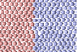
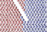
The apex of the triangle in figure 6 is a perfect crystal oriented at 30∘, which is the end point of a series of symmetric tilt boundaries. At exactly , there is an abrupt jump up in fracture strength since the perfect crystal has no “extra dislocations” at which to nucleate fracture. Our simulations find a peak stress of 4.31 (Lennard-Jones Units) for the perfect crystal.
The low angle grain boundaries near the 30∘ lattice orientation have surface vectors and , repeat distances , and total Burger’s vector , which splits into two flaws with Burger’s vectors and shown in figure 13. For wide enough simulations, these dislocations glide in opposite directions until they are restricted by the constrained zones on either side. For narrower simulations, the dislocations do not glide but form nucleation points for grain boundary fracture causing an abrupt jump down in the peak stress compared to the peak stress of the perfect crystal.


For narrow simulations of low angle grain boundaries in this region, we find that the peak stress has a parabolic dependence on angle, shown in figure 14. We can explain this parabolic dependence as due to a partial screening of the external stress by the neighboring dislocations on the grain boundary. Assume that the dislocation has a critical stress for nucleating fracture equal to . The dislocation feels a stress due to its neighboring dislocations, each a distance apart, in addition to the external, applied stress. The total stress felt by each dislocation can be written
| (7) |
where is the external stress. The term is the Volterra solution given by
| (8) | |||||
| (9) | |||||
| (10) |
where the -direction is the direction of the Burger’s vector. Since the Volterra solution is odd, the term of the stress at each dislocation vanishes as we sum over the neighboring dislocations on either side. The first nonvanishing term in equation 7 is the term which has three contributions. (1) The terms are the multiple expansions of the stress field Bailey 2002 as well as nonlinear terms. (2) The nonlinear term in strain field has the form , giving a power law of . (3) Geometrical restrictions cause some grain boundaries to have flaws unequally spaced in the -direction (though for the results given in figure 14 we have only explored geometries with equally spaced flaws). The grain boundaries geometries used in figure 14 do have flaws that are not aligned perfectly in the -direction. In each of these cases, shifting the dislocation constitutes adding a dislocation dipole (adding one positive and one negative, canceling a dislocation and adding a new one), and therefore is another contribution to the term. The external stress needed to produce a stress equal to at each flaw is then
| (11) |
where combines the three contributions described above. This parabolic dependence on is depicted on the left-hand side of figure 15.
V.2 High Angle Grain Boundaries
Figure 15 shows the results of the peak stress measurements for high angle symmetric grain boundaries. At the same points for which we had cusps in energy, we have discontinuous increases in fracture strength. By drawing the same analogy between adding dislocations to perfect crystals and adding flaws to high symmetry boundaries as described in figure 8 we can understand the discontinuities in the fracture strength at high symmetry grain boundaries and the angular dependence of fracture strength near the high symmetry geometries.

For high angle grain boundaries, the added flaw is no longer the sole nucleation site for fracture and fracture does not necessarily nucleate in the core of the added flaw. The added dislocation creates a stress field given roughly by the Volterra solution (equation 10) with a positive stress on one side, negative stress on the other, and a singularity at the center shown in figure 16. The stress field differs slightly from the Volterra solution because the elastic constants of the material at the grain boundary vary from those of the perfect crystal. The fracture nucleates along the boundary in the region where the stress due to the added flaw is positive. Because fracture does not nucleate at the center of the added flaw, the Volterra solution as summed over the neighboring, added flaws does not cancel at the nucleation site. This leads to a linear law for fracture strength as a function of tilt angle, for grain boundaries near high symmetry geometries.


Consider the grain boundaries with tilt angles ranging from 49.39∘ to 53.41∘, which are close to the high symmetry grain boundary at 49.11∘. The additional flaws that characterize these grain boundaries have Burger’s vectors equal to and , where is the symmetric tilt angle of the lattice. The norms are and the angles are 210 and 150∘. For these geometries, the component of the stress field (due to two dislocations a distance ) along the -axis is
| (12) | |||||
| (13) |
where is the tilt angle of the high symmetry grain boundary. We need to look at simulations in the fixed displacement (narrow width) regime in order to observe where fracture nucleates. 66 6 For simulations of a few angstroms wide, the crack opens up along the grain boundary with a slow unzipping mechanism, starting at particular flaws. For wider simulations, the crack snaps open, soon after a peak stress is reached. The slow unzipping of the narrow simulations is characteristic of fixed displacement boundary conditions - since the displacements of a region close to the interface is fixed, the opening of the crack is controlled, allowing us to see the details of how the crack opens. The snapping open, seen with a wider simulation, is characteristic of fixed force boundary conditions. In the wider simulations, the material on either side of the grain boundary acts as a spring, which effectively softens the boundary conditions, approximating fixed-force boundaries for long lengths. When the constrained region is far away, the interface snaps open once it reaches the maximum stress that it can sustain. We find that for geometries with this pattern of flaws, fracture nucleates at the same distance above the added flaw. The external stress needed to nucleate fracture at a distance y from the added flaw, along the grain boundary is then approximately
| (14) |
which explains the linear dependence on angle shown in figures 16 and 17.


The results for the peak stress of all grain boundaries with repeat lengths less than 30 lattice constants are shown in figure 18. We also note spikes in peak stress for grain boundaries with particularly low repeat distances. Consider again the grain boundary with tilt angles 24.79∘ and 3.00∘ which has a repeat distance of 9.53 lattice constants. Figure 19 shows the peak stress of this grain boundary and grain boundaries in its neighborhood, along a line of constant misorientation.
VI Conclusion
We have systematically explored the space of 2D grain boundaries, the patterns of structural units that make up short repeat distance grain boundaries, and the flaws in the patterns of structural units that make up vicinal grain boundaries. We have shown that the patterns of structural units are key to understanding the singularities in energy and peak stress at special grain boundaries by drawing an analogy to perfect crystals. We have used this insight to find a functional form for the energies of 2D symmetric grain boundaries and to understand the tilt angle dependence of peak stress near special grain boundaries.
In principle, with enough computer time it would be possible to conduct a similar study for the 5D space of idealized 3D grain boundaries. We suspect that the perfect crystal analogy could also explain the cusps in energy and discontinuous spikes in peak stress for special 3D grain boundaries. The geometry dependence of energy and peak stress surrounding these special grain boundaries will be more complicated since the grain boundaries can have a pure tilt, pure twist, or a mixed type of geometry. In real polycrystals, the fracture strength and energy are further complicated by impuritites at the interface, emission of dislocations during fracture, and more complex geometries such as triple junctions of grains, which are often the nucleation site for fracture. Systematic studies of such systems are infeasible and better suited by on the fly simulations of local regions of interest.
Acknowledgements.
This work was supported by NSF Grants No. ITR/ASP ACI0085969 and No. DMR-0218475. We also wish to thank Nicholas Bailey, Drew Dolgert, Gerd Heber, Anthony Ingraffea, Surachute Limkumnerd, Chris Myers, and Paul Wawrzynek.References
- Needleman (1990) A. Needleman, Journal of the Mechanics and Physics of Solids 38, 289 (1990).
- Falk et al. (2001) M. Falk, A. Needleman, and J. Rice, in Pro-ceedings of the 5th European Mechanics of Materials Conference (Delft, 2001), URL http://citeseer.ist.psu.edu/490781.html.
- Iesulauro et al. (2002) E. Iesulauro, A. R. Ingraffea, S. Arwade, and P. A. Wawrzynek, in Fatigue and Fracture Mechanics, edited by W. G. Reuter and R. S. Piascik (American Society for Testing and Materials, West Conshohocken, PA, 2002), vol. 33.
- Iesulauro et al. (2003) E. Iesulauro, A. R. Ingraffea, G. Heber, and P. A. Wawrzynek, in 44th AIAA/ASME/ASCE/AHS Structures, Structural Dynamics, and Materials Conference (AIAA, Norfolk, VA, 2003).
- Warner et al. (2006) D. H. Warner, F. Sansoz, and J. F. Molinari, International Journal of Plasticity 22, 754 (2006).
- Coffman et al. (2007) V. R. Coffman, J. P. Sethna, G. Heber, A. Liu, A. Ingraffea, and E. I. Barker (2007), in preparation.
- Chen et al. (1989) S. P. Chen, D. J. Srolovitz, and A. F. Voter, Journal of Materials Research 4, 62 (1989).
- Sansoz and Molinari (2004) F. Sansoz and J. F. Molinari, Scripta Materialia 50, 1283 (2004).
- Sansoz and Molinari (2005) F. Sansoz and J. F. Molinari, Acta Materialia 53, 1931 (2005).
- Shenderova et al. (2000) O. A. Shenderova, D. W. Brenner, A. Omeltchenko, X. Su, and L. H. Yang, Phys. Rev. B 61, 3877 (2000).
- Spearot et al. (2004) D. E. Spearot, K. I. Jacob, and D. L. McDowell, Mechanics of Materials 36, 825 (2004).
- Bollmann (1970) W. Bollmann, Crystal Defects and Crystalline Interfaces (Springer-Verlag, New York, 1970).
- Bishop and Chalmers (1968) G. H. Bishop and B. Chalmers, Scripta Metallurgica 2, 133 (1968).
- Ishida (1976) Y. Ishida, Grain Boundary Structure and Properties (Academic Press Inc., London, 1976), chap. The Bubble Raft as a Model for Grain Boundary Structure, pp. 93–106.
- Wolf and Merkle (1992) D. Wolf and K. L. Merkle, Materials Interfaces: Atomic-level structure and properties (Chapman & Hall, 1992), chap. Correlation between the structure and energy of grain boundaries in metals, pp. 88–150.
- Harrison et al. (1976) R. J. Harrison, G. A. Bruggeman, and G. H. Bishop, Grain Boundary Structure and Properties (Academic Press Inc., London, 1976), chap. Computer Simulation Methods applied to Grain Boundaries, pp. 45–91.
- Pumphrey (1976) P. H. Pumphrey, Grain Boundary Structure and Properties (Academic Press Inc., London, 1976), chap. Special High Angle Grain Boundaries, pp. 139–200.
- Wolf (1992) D. Wolf, Materials Interfaces: Atomic-level structure and properties (Chapman & Hall, 1992), chap. Atomic-level geometry of crystalline interfaces, pp. 1–52.
- Wolf and Jaszczak (1992) D. Wolf and J. A. Jaszczak, Materials Interfaces: Atomic-level structure and properties (Chapman & Hall, 1992), chap. Role of interface dislocations and surface steps in the work of adhesion, pp. 662–690.
- Hirth and Lothe (1982) J. P. Hirth and J. Lothe, Theory of Dislocations (John Wiley & Sons, New York, 1982).
- Bailey et al. (2006) N. Bailey, T. Cretegny, J. P. Sethna, V. R. Coffman, A. J. Dolgert, C. R. Myers, J. Schiotz, and J. J. Mortensen, Digital material: a flexible atomistic simulation code (2006), URL http://arxiv.org/abs/cond-mat/0601236.
- Palumbo and Aust (1992) G. Palumbo and K. T. Aust, Materials Interfaces: Atomic-level structure and properties (Chapman & Hall, 1992), chap. Special Properties of grain boundaries., pp. 190–207.
- Bailey (2002) N. Bailey, Ph.D. thesis, Cornell (2002).
- Allen and Tildesley (1987) M. P. Allen and D. J. Tildesley, Computer Simulation of Liquids (Oxford Science Publications, 1987).
- Frenkel and T. (1938) Y. I. Frenkel and K. T., Zhurnal tekhnicheskoi fiziki 8, 1340 (1938).