Risk Analysis in Robust Control — Making the Case for Probabilistic Robust Control Thanks: This research is supported in part by the US Air Force.
The authors are with Department of Electrical and Computer Engineering, Louisiana State University, Baton Rouge, LA 70803; Email: {chan,kemin, aravena}@ece.lsu.edu, Tel: (225)578-{8961, 5533,5537}, and Fax: (225) 578-5200.

Xinjia Chen Jorge L. Aravena Kemin Zhou

June 2007

Abstract

This paper offers a critical view of the “worst-case” approach that is the cornerstone of robust control design. It is our contention that a blind acceptance of worst-case scenarios may lead to designs that are actually more dangerous than designs based on probabilistic techniques with a built-in risk factor. The real issue is one of modeling. If one accepts that no mathematical model of uncertainties is perfect then a probabilistic approach can lead to more reliable control even if it cannot guarantee stability for all possible cases. Our presentation is based on case analysis. We first establish that worst-case is not necessarily “all-encompassing.” In fact, we show that for some uncertain control problems to have a conventional robust control solution it is necessary to make assumptions that leave out some feasible cases. Once we establish that point, we argue that it is not uncommon for the risk of unaccounted cases in worst-case design to be greater than that of the accepted risk in a probabilistic approach. With an example, we quantify the risks and show that worst-case can be significantly more risky. Finally, we join our analysis with existing results on computational complexity and probabilistic robustness to argue that the deterministic worst-case analysis is not necessarily the better tool.

1 Introduction

In recent years, a number of researchers have proposed probabilistic control methods as alternatives for overcoming the computational complexity and conservatism of deterministic worst-case robust control framework (e.g., [1]–[33], [35]–[43] and the references therein). The philosophy of probabilistic control theory is to sacrifice extreme cases of uncertainty. Such paradigm has lead to the novel concepts of probabilistic robustness margin and confidence degradation function (e.g., [2]). Despite the claimed advantages of probabilistic approach, the deterministic worst-case approach remains dominating for design and analysis purposes. It is a common contention that a probabilistic design is more risky than a worst-case design. Such a contention may have been the main obstacle preventing the wide acceptance of the probabilistic paradigm, especially in the development of highly reliable systems. When referring to the probabilistic approach, a cautious warning is usually attached. Statements like “if one is willing to accept a small risk of performance violation” can be found in a number of robust control papers. A typical argument is that the worst-case method takes every case of “uncertainty” into account and is certainly the most safe, while the probabilistic method considers only most of the instances of “uncertainty” and, hence, is more risky.

We illustrate with two very simple cases that a worst case design may not necessarily consider all possible cases. Our purpose here is to make the point that the basic issue is one of modeling and as such it is never perfect. Worst-case scenario may mean “the worst case that we can imagine,” or “the worst-case that we can afford to consider to have a robust solution.”

In practice, the coefficients of a linear model are complex functions of physical parameters. Even if the physical parameters are bounded in a narrow interval, the variations of the coefficients can be fairly large. A simple example is provided by the process of discharge of a cylindrical tank. The basic nonlinear model is of the form

A\frac{dH}{dt}+\rho\sqrt{H}=Q_{i}

where $A$ is the tank cross section, $H$ the height of liquid inside the tank, $Q_{i}$ the volumetric input flow rate and $\rho$ the hydraulic resistance in the discharge. Linearizing in the neighborhood of a steady state operating point, ( $\overline{H},\overline{Q}_{i}$ ), satisfying $\rho\sqrt{\overline{H}}=\overline{Q_{i}}$ one obtains the linear model

\frac{dh}{dt}+\frac{\rho}{2A\sqrt{\overline{H}}}h=\frac{q_{i}}{A}

with $h=H-\overline{H},q_{i}=Q_{i}-\overline{Q}_{i}$ . Clearly, the parameter $a=\frac{\rho}{2A\sqrt{\overline{H}}}$ takes values in the interval ( $0,~\infty$ ). Hence, any design assuming bounded uncertainties for the parameter, $a$ , cannot include all possible heights for the liquid.

For the second case consider a first order system of the form

G(s)=\frac{q}{s-p}

with uncertain parameters $q$ and $p$ . Assuming a unity feedback and controller of the form

C(s)=\frac{K}{s+a},\quad K>0,\quad a>0

the closed loop system becomes

T(s)=\frac{Kq}{s^{2}+(a-p)s+Kq-ap}.

The controller will robustly stabilize the plant if

p<a,\qquad q>\frac{ap}{K}.

It is clear that for any finite controller gain $K$ , there exist a range of values of $q$ where the closed-loop system is unstable. The designer of a worst-case controller would be faced with the choice of selecting a different controller structure or assuming, based on other considerations, that a neighborhood of $q=0$ can be excluded from the design. With the next result we develop this point in a more general form.

1.1 Uncertainties in Modeling Uncertainties

In many practical situations of worst-case design one models uncertainties as bounded random variables. The issue of selecting the bounds is not trivial and is, oftentimes, not addressed in detail. The following theorem shows that, regardless of the assumed size of the uncertainty set, a worst-case robust controller actually can always fail. Hence, if there are “uncertainties in modeling the uncertainties” it may be better to model them as random variables varying from $-\infty$ to $\infty$ in order to pursue “worst-case” in a strict sense.

Theorem 1

Let the transfer function of the uncertain plant be

G(s)=\frac{\sum_{i=0}^{\ell}\beta_{i}s^{\ell-i}}{\sum_{i=0}^{\kappa}\alpha_{i}s^{\kappa-i}},\qquad\alpha_{0}=1,\qquad\ell\leq\kappa.

Assume that for a given finite uncertainty range in the parameters $\alpha_{i},\;i=1,\cdots,\kappa$ and $\beta_{j},\;j=0,1,\cdots,\ell$ , there exists a controller of the form

C(s)=\frac{\sum_{i=0}^{m}b_{i}s^{m-i}}{\sum_{i=0}^{n}a_{i}s^{n-i}},\qquad a_{0}=1,\qquad b_{0}\neq 0,\qquad m\leq n

which robustly stabilizes the system. Then, there always exists a value of parameter $\alpha_{i}$ or $\beta_{j}$ , outside the assumed uncertainty range and which will make the closed-loop system unstable.

Proof.

The characteristic equation of the closed-loop system is

\left(\sum_{i=0}^{n}a_{i}s^{n-i}\right)\;\left(\sum_{j=0}^{\kappa}\alpha_{j}s^{\kappa-j}\right)+\left(\sum_{i=0}^{m}b_{i}s^{m-i}\right)\;\left(\sum_{j=0}^{\ell}\beta_{j}s^{\ell-j}\right)=0,

which can be written as

\sum_{\tau=0}^{n+\kappa}\sum_{i+j=\tau\atop{0\leq i\leq n\atop{0\leq j\leq\kappa}}}(a_{i}\;\alpha_{j})\;s^{n+\kappa-\tau}+\sum_{\iota=0}^{m+\ell}\sum_{i+j=\iota\atop{0\leq i\leq m\atop{0\leq j\leq\ell}}}(b_{i}\;\beta_{j})\;s^{m+\ell-\iota}=0.

For $1\leq\tau\leq\kappa$ , the coefficient of $s^{n+\kappa-\tau}$ is

\sum_{i+j=\tau\atop{0\leq i\leq n\atop{0\leq j\leq\kappa}}}(a_{i}\;\alpha_{j})+\sum_{i+j=\tau+m+\ell-(n+\kappa)\atop{0\leq i\leq m\atop{0\leq j\leq\ell}}}(b_{i}\;\beta_{j})=\alpha_{\tau}+\xi

where

	$\displaystyle\xi$	$\displaystyle=$	$\displaystyle\sum_{i+j=\tau\atop{1\leq i\leq n\atop{0\leq j\leq\kappa}}}(a_{i}\;\alpha_{j})+\sum_{i+j=\tau+m+\ell-(n+\kappa)\atop{0\leq i\leq m\atop{0\leq j\leq\ell}}}(b_{i}\;\beta_{j})$
		$\displaystyle=$	$\displaystyle\sum_{j=\max(0,\tau-n)}^{\tau-1}(a_{\tau-j}\;\alpha_{j})+\sum_{i+j=\tau+m+\ell-(n+\kappa)\atop{0\leq i\leq m\atop{0\leq j\leq\ell}}}(b_{i}\;\beta_{j})$

is independent of $\alpha_{\tau}$ and depends on the other uncertainties. It follows that the system will be unstable if

\alpha_{\tau}\leq-\xi.

(1)

In a similar manner, for $0\leq\iota\leq\ell$ , the coefficient of $s^{m+\ell-\iota}$ is

\sum_{i+j=\iota\atop{0\leq i\leq m\atop{0\leq j\leq\ell}}}(b_{i}\;\beta_{j})+\sum_{i+j=\iota+n+\kappa-(m+\ell)\atop{0\leq i\leq n\atop{0\leq j\leq\kappa}}}(a_{i}\;\alpha_{j})=b_{0}\;\beta_{\iota}+\zeta

where

	$\displaystyle\zeta$	$\displaystyle=$	$\displaystyle\sum_{i+j=\iota\atop{1\leq i\leq m\atop{0\leq j\leq\ell}}}(b_{i}\;\beta_{j})+\sum_{i+j=\iota+n+\kappa-(m+\ell)\atop{0\leq i\leq n\atop{0\leq j\leq\kappa}}}(a_{i}\;\alpha_{j})$
		$\displaystyle=$	$\displaystyle\sum_{j=\max(0,\iota-m)}^{\iota-1}(b_{\iota-j}\;\beta_{j})+\sum_{i+j=\iota+n+\kappa-(m+\ell)\atop{0\leq i\leq n\atop{0\leq j\leq\kappa}}}(a_{i}\;\alpha_{j})$

is independent of $\beta_{\iota}$ and depends on the other uncertainties. It follows that the system will be unstable if

b_{0}\;\beta_{\iota}+\zeta\leq 0.

(2)

In the case that $b_{0}>0$ , the system is unstable when $\beta_{\iota}\leq-\frac{\zeta}{b_{0}}$ . In the case that $b_{0}<0$ , the system is unstable when $\beta_{\iota}\geq-\frac{\zeta}{b_{0}}$ .

Let $\cal{B}$ be the uncertainty bounding set assumed by the designer. Let $\cal{D}$ be the set of all values of uncertainties for which the controller stabilizes the system. Obviously, $\cal{B}\subseteq\cal{D}$ . From the stability conditions (1) and (2), we can conclude that $\cal{D}$ must be bounded. Taking into account the stability conditions and the fact that $\cal{D}$ is bounded, we can see that there exist values of the parameters $\alpha_{i},\;1\leq i\leq\kappa$ or $\beta_{j},\;0\leq j\leq\ell$ that fall outside the domain $\cal{D}$ (of course they fall outside the assumed uncertainty range $\cal{B}$ ) and make the system unstable.

$\Box$

Remark 1

A proof for an equivalent result for a multi-variable plant may be feasible. However, the following general argument conveys the idea about the limitations in worst case design. Assume that each instance of uncertainty is an element of $n$ -dimensional vector space $E^{n}$ . Let $G(s,q),\;q\in\cal{B}\subset E^{n}$ be the model for an uncertain plant. Assume that there exists a controller $C_{w}$ that satisfies the robustness requirements for all $q\in\cal{B}$ . Define now as $\cal{D}$ the set of all values of the parameter $q$ where the controller $C_{w}$ satisfies the robustness requirements. Clearly $\cal{D}_{w}\supset\cal{B}$ but unless $\cal{D}_{w}=E^{n}$ there always exist values of the parameter $q$ where the controller does not perform. The worst-case design ignores these cases as impossible. Our contention is that the modeling of uncertainties (the set $\cal{B}$ ) may not include all cases that could occur and it may be better to accept a risk from the onset of the design.

2 Accepting Risk Can Be Less Risky

The previous result makes, very strongly, the point that worst-case modeling is not “all-encompassing” and therefore it has some risk associated to it. In this section we offer first a more formal description of the problem and argue that a probabilistic approach may easily lead to more reliable designs. The next section uses a case study to quantify the actual risks of both approaches.

2.1 Designing with Uncertain Uncertainties

We incorporate the fact that modeling is never exact by postulating an uncertainty set, $\cal{U}$ and a bounding set, $\cal{B}$ , that models the uncertainties. The actual relationship between the two sets is not known. The worst-case design finds a controller $C_{w}$ to guarantee every uncertainty instance $q\in\cal{B}$ . The probabilistic design seeks a controller $C_{p}$ to guarantee most uncertainty instances $q\in\cal{B}$ . Formally we can define the following relevant subsets

$\displaystyle\cal{M}$	$\displaystyle=$	$\displaystyle\cal{U}\cap\cal{B},$
$\displaystyle\cal{N}$	$\displaystyle=$	$\displaystyle\overline{\cal{U}}\cap\cal{B},$
$\displaystyle\cal{E}$	$\displaystyle=$	$\displaystyle\cal{U}\cap\overline{\cal{B}}.$

Here $\overline{X}$ denotes the complementary set of $X$ . Clearly, $\cal{M}$ contains those uncertainties that are modeled while the set $\cal{N}$ describes modeled uncertainties that never occur and $\cal{E}$ describes the unmodeled uncertainties. The existence of these last two sets creates either inefficiencies or risks in the worst case design. To see this, consider the extreme situation where the designed robust controller guarantees the robustness requirement only for instances in $\cal{B}$ . The controller is over-designed because it deals with situations that cannot occur and it has the risk of failure if an instance in the set $\cal{E}$ arises.

Having established the fact that a robust control design can be risky, we now argue that probabilistic design can actually be less risky. As an added benefit, it is known that many worst-case synthesis problems are either not tractable, or have known solutions which are unduly conservative and implementation expensive. But when using a probabilistic method, the previously intractable problems may become solvable, the conservatism may be overcame, and high performance controller with simple structure may be obtained.

For brevity, we use notation $C^{V}$ to represent the statement that “the robustness requirement is violated for the system with controller $C$ ”. The subindex $w$ will refer to worst-case design while $p$ will refer to probabilistic design. Note that the risk of a probabilistic design is

P_{e}^{p}=\Pr\{C^{V}_{p}\mid q\in\cal{M}\}\;\Pr\{q\in\cal{M}\}+\Pr\{C^{V}_{p}\mid q\in\cal{E}\}\;\Pr\{q\in\cal{E}\}.

While the risk of a worst-case design is

P_{e}^{w}=\Pr\{C^{V}_{w}\mid q\in\cal{E}\}\;\Pr\{q\in\cal{E}\}.

Hence the ratio of risks will be

\frac{P_{e}^{p}}{P_{e}^{w}}=\frac{\Pr\{C^{V}_{p}\mid q\in\cal{E}\}}{\Pr\{C^{V}_{w}\mid q\in\cal{E}\}}+\frac{\Pr\{C^{V}_{p}\mid q\in\cal{M}\}\Pr\{q\in\cal{M}\}}{\Pr\{C^{V}_{w}\mid q\in\cal{E}\}\Pr\{q\in\cal{E}\}}.

(3)

The first term is related to the performance of both types of controllers outside the design region. The behavior of the worst-case design in this region is of no concern to the designer, after all it “never gets there.” All the design effort is placed in assuring performance over the set $\cal{B}$ . Hence we can reasonably expect $\Pr\{C^{V}_{w}\mid q\in\cal{E}\}$ to be high. In fact, if the set $\cal{N}$ , of impossible situations included in the design, is large then $\Pr\{C^{V}_{w}\mid q\in\cal{E}\}$ could be close to one and the first term in the right-hand side of (3) can easily be less than some number $\lambda\in(0,1)$ . The second term contains the factor $\Pr\{C^{V}_{p}\mid q\in\cal{M}\}$ which is under the probabilistic designer and is a measure of the accepted risk. It is reasonable to expect that this risk is less than $\Pr\{q\in\cal{E}\}$ so that

\displaystyle\frac{\Pr\{C^{V}_{p}\mid q\in\cal{M}\}\Pr\{q\in\cal{M}\}}{\Pr\{q\in\cal{E}\}}<(1-\lambda)\;\Pr\{C^{V}_{w}\mid q\in\cal{E}\}.

and consequently $\frac{P_{e}^{p}}{P_{e}^{w}}<1$ . Factoring in a poor performance for the worst-case design outside of the modeled region one can see that the risk of the probabilistic design can become smaller than the risk of a worst-case design with unmodeled uncertainties.

From a different point of view, many experiments of performance degradation of probabilistic designs indicate a fairly flat characteristic. If the unmodeled uncertainty set $\cal{E}$ is relatively small then one could argue that

\displaystyle\Pr\{C^{V}_{p}\mid q\in\cal{E}\}\approx\Pr\{C^{V}_{p}\mid q\in\cal{M}\}

and the ratio of risks is approximately given by

\frac{P_{e}^{p}}{P_{e}^{w}}\approx\frac{\Pr\{C^{V}_{p}\mid q\in\cal{M}\}}{\Pr\{C^{V}_{w}\mid q\in\cal{E}\}\Pr\{q\in\cal{E}\}}.

(4)

The numerator is under the control of the designer in a probabilistic approach while the denominator has not even been considered as existing in a worst-case design.

3 Comparing Worst-Case and Probabilistic Designs

The problem of quantifying the differences in performance between a worst-case design and a probabilistic design is extremely difficult in general. In this section we use a case study to quantify the risks and demonstrate that it is not uncommon for a probabilistic controller to be (highly) more reliable than a worst-case controller. We postulate that if the result holds for simple systems then it is also likely for more complex situations.

Consider a feedback system as follows.

Figure 1: Standard Feedback Configuration

The transfer function of the plant is

G(s)=\frac{q}{s-p}

where $p$ and $q$ are uncertain parameters. These parameters are assumed as independent Gaussian random variables with density $\cal{N}(q_{0},\sigma_{q})$ and $\cal{N}(p_{0},\sigma_{p})$ respectively and

p_{0}<0,\qquad q_{0}>0

(5)

For the worst case design it is assumed that $(q,p)\in\cal{B}(r)$ where

\cal{B}(r)=\{(x,y)\mid\;|x-q_{0}|\leq r,\quad|y-p_{0}|\leq r\}

is the uncertainty bounding set with radius $r>0$ . We use $P^{\mathrm{Box}}$ to denote $\Pr\{(q,p)\in\cal{B}(r)\}$ , i.e., the coverage probability of the uncertainty bounding set. It can be shown that

P^{\mathrm{Box}}=\mathrm{erf}\left(\frac{r}{\sqrt{2}\;\sigma_{p}}\right)\mathrm{erf}\left(\frac{r}{\sqrt{2}\;\sigma_{q}}\right)

where

\mathrm{erf}(x)\stackrel{{\scriptstyle\mathrm{def}}}{{=}}\frac{2}{\sqrt{\pi}}\int_{0}^{x}e^{-t^{2}}dt.

Hence, by increasing the radius $r$ , one can reduce the uncertainty modeling error.

Consider two controllers

C_{A}=\frac{K_{A}}{s+a},\qquad a>0

and

C_{B}=K_{B}.

We assume further that

1<K_{B}<\frac{K_{A}}{a}.

(6)

When using controller $C_{A}$ , the closed-loop transfer function is given by

T=\frac{\frac{K_{A}}{s+a}\frac{q}{s-p}}{1+\frac{K_{A}}{s+a}\frac{q}{s-p}}=\frac{K_{A}q}{s^{2}+(a-p)s+K_{A}q-ap}

which is stable if and only if

p<a,\qquad p<\frac{K_{A}}{a}q.

The deterministic stability margin of the system is given by

\rho_{A}=\sup\left\{r>0\mid p_{0}+r<\frac{K_{A}}{a}(q_{0}-r),\quad p_{0}+r<a\right\}

which can be simplified as

\rho_{A}=\min\left(\frac{K_{A}\;q_{0}-a\;p_{0}}{K_{A}+a},\;a-p_{0}\right).

When using controller $C_{B}$ , the closed-loop transfer function is given by

T=\frac{K_{B}\;q}{s+K_{B}\;q-p}

which is stable if and only if

p<K_{B}\;q.

The deterministic stability margin of the system is given by

	$\displaystyle\rho_{B}$	$\displaystyle=$	$\displaystyle\sup\left\{r>0\mid p_{0}+r<K_{B}(q_{0}-r)\right\}$
		$\displaystyle=$	$\displaystyle\frac{K_{B}\;q_{0}-p_{0}}{K_{B}+1}.$

For uncertainty bounding set with radius $r\in(\rho_{B},\;\rho_{A})$ , i.e.,

\frac{K_{B}\;q_{0}-p_{0}}{K_{B}+1}<r<\min\left(\frac{K_{A}\;q_{0}-a\;p_{0}}{K_{A}+a},\;a-p_{0}\right),

(7)

controller $B$ may make the system unstable while controller $A$ robustly stabilizes the system. More specifically, controller $B$ can only stabilize a proportion of the family of uncertain plants. Such a proportion, denoted by $\mathbb{P}(r)$ , is referred to as proportion of stability, which is computed as the ratio of the volume of the set of parameters making the system stable to the total volume of the uncertainty box, i.e.,

\mathbb{P}(r)=\frac{\mathrm{vol}\{(q,p)\in\cal{B}(r)\mid\text{The system is stable for $(q,p)$}\}}{\mathrm{vol}\{\cal{B}(r)\}}.

Here “ $\mathrm{vol}$ ” denotes the Lebesgue measure. More details are given in Appendix A where we show that the proportion of instability for controller $B$ is given by

\mathbb{P}^{B}(r)=\begin{cases}1&\text{for}\quad 0<r<\rho_{B};\\ 1-\frac{K_{B}\left(r+\frac{p_{0}+r}{K_{B}}-q_{0}\right)^{2}}{8r^{2}}&\text{for}\quad\rho_{B}\leq r\leq\rho_{B}^{*};\\ \frac{1}{2}-\frac{\frac{p_{0}}{K_{B}}-q_{0}}{2r}&\text{for}\quad r>\rho_{B}^{*}\end{cases}

(8)

with

\rho_{B}^{*}=\frac{K_{B}\;q_{0}-p_{0}}{K_{B}-1}.

For an uncertainty bounding set with radius $r\in(\rho_{B},\;\rho_{A})$ , controller $B$ is actually a probabilistic controller because its proportion of stability is strictly less than $1$ . Obviously, controller $A$ is a worst-case controller and is naturally considered to be more reliable than the probabilistic controller $B$ . However, the following exact computation of probabilities of instability for both controllers reveals that the worst-case controller can actually be substantially more risky than the probabilistic controller.

We use $P^{C_{A}}$ to denote $\Pr\{\text{Controller $C_{A}$ de-stabilizes the system}\}$ . We have derived an exact expression as

P^{C_{A}}=\frac{1}{2\pi}\left[\int_{\theta=0}^{\theta^{*}}\exp\left(-\frac{u^{2}}{2\sin^{2}\theta}\right)d\theta+\int_{\theta=\theta^{*}-\arctan(k)}^{\pi}\exp\left(-\frac{w^{2}}{2\sin^{2}\theta}\right)d\theta\right]

(9)

where

u=\frac{a-p_{0}}{\sigma_{p}}>0,\qquad v=\frac{\frac{K_{A}}{a}q_{0}-p_{0}}{\sigma_{p}}>0,\qquad k=\frac{K_{A}}{a}\frac{\sigma_{q}}{\sigma_{p}},\qquad w=\frac{v}{\sqrt{1+k^{2}}}

and

\theta^{*}=\arctan\left(\frac{ku}{u-v}\right)\in(0,\pi).

For a proof of formula (9), see Appendix B.

We use $P^{C_{B}}$ to denote $\Pr\{\text{Controller $C_{B}$ de-stabilizes the system}\}$ . We have derived an exact expression as

P^{C_{B}}=\frac{1}{2}-\frac{1}{2}\;\mathrm{erf}\left(\frac{K_{B}q_{0}-p_{0}}{\sqrt{2(\sigma_{p}^{2}+K_{B}^{2}\sigma_{q}^{2})}}\right).

(10)

For a proof of formula (10), see Appendix C.

A sufficient (but not necessary) condition for the worst-case controller to be more risky than the probabilistic controller (i.e., $P^{C_{A}}>P^{C_{B}}$ ) is

1+\left(\frac{K_{B}\;\sigma_{q}}{\sigma_{p}}\right)^{2}<\left(\frac{K_{B}q_{0}-p_{0}}{a-p_{0}}\right)^{2},

(11)

which can be easily satisfied. For a derivation of condition (11), see Appendix D.

The boundary of stability is shown in Figure 2.

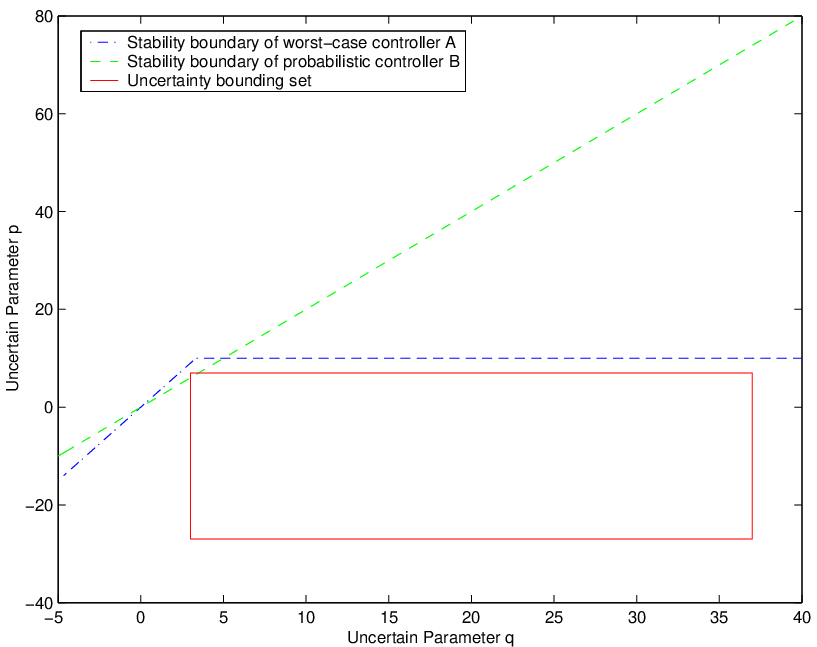
Refer to caption — Figure 2: Comparison of worst-case controller and probabilistic controller ( $r=17,\;a=10,\;p_{0}=-10,\;q_{0}=20,\;K_{A}=30,\;K_{B}=2,\;\sigma_{p}=10,\;\sigma_{q}=5$ )

In Table $1$ we compute the ratio of probabilities of being unstable for both the worst-case and probabilistic designs for several situations. The results show that a worst-case controller can be thousands of times more risky than a probabilistic controller. Granted that this is a simple first order system but our contention is that if it happens even for this simple case then the situation can (easily) happen for highly complicated systems.

Table 1: Comparison of risks (

\rho_{B}<r<\rho_{A}

)

$a$	$r$	$p_{0}$	$q_{0}$	$\sigma_{p}$	$\sigma_{q}$	$K_{A}$	$K_{B}$	$P^{\mathrm{Box}}$	$\mathbb{P}^{B}(r)$	$P^{C_{A}}$	$\frac{P^{C_{A}}}{P^{C_{B}}}$
$10$	$17$	$-10$	$20$	$10$	$5$	$30$	$2$	$0.91$	$0.9998$	$2.3\times 10^{-2}$	$112$
$40$	$49$	$-10$	$50$	$20$	$10$	$4000$	$10$	$0.99$	$0.9956$	$6.2\times 10^{-3}$	$2.2\times 10^{4}$

It has been the consensus in the field that guarantees with certainty are often required for stability and performance in control, while the probabilistic design is a viable approach when only probabilistic guarantees are required (see, e.g., lines 16-25, page 4652 of [34]). From our general arguments and the concrete example, we can see that, in a strict sense, “guarantees with certainty” are only possible within the modeled uncertainty bounding set. Our contention is that such worst-case guarantees may not imply better robustness than probabilistic guarantees because of the fact the uncertainty bounding set may not include all instances of uncertainty.

4 Conclusion

In this paper, we demonstrate that the deterministic worst-case robust control design does not necessarily imply a risk free solution and that, in fact, it can be more risky than a probabilistic controller. In the final instance, every design and analysis is subject to a level of risk. The goal of design should be to make the risk acceptable, instead of assuming that it can make it vanish.

It has been acknowledged that probabilistic methods overcome the computational complexity and conservatism of worst-case approach at the expense of a probabilistic risk ([10], p. 1908). In fact has been remarked by Kargonekar and Tikku that if one is willing to draw conclusions with a high degree of confidence, then the computational complexity decreases dramatically ([20], p. 3470). More formally, let $\epsilon,\delta\in(0,1)$ and define a system to be $\epsilon$ -non-robust if

\frac{\mathrm{vol}(\{q\in\mathcal{B}\mid\mathbf{P}\;\mathrm{is\;violated\;for}\;q\})}{\mathrm{vol}(\mathcal{B})}\geq\epsilon.

Then one can detect any $\epsilon$ -non-robust system with probability greater than $1-\delta$ based on $N>\frac{\ln\frac{1}{\delta}}{\ln\frac{1}{1-\epsilon}}$ i.i.d. simulations [20, 38].

Recently, Barmish et. al. pointed out that if one is willing to accept some small risk probability of performance violation, it is often possible to expand the radius of allowable uncertainty by a considerable amount beyond that provided by the classical robustness theory ([2], p. 853).

Putting these last two statements in the light of our result make a strong case for the use of probabilistic robustness methods.

Appendix A Proportion of Instability of Probabilistic Controller

The set of values uncertainties bounded in $\cal{B}(r)$ which make the system unstable is

\cal{B}^{\mathrm{Bad}}(r)=\{(x,y)\mid\;y\geq K_{B}\;x,\quad|x-q_{0}|\leq r,\quad|y-p_{0}|\leq r\}.

(12)

Clearly,

\mathbb{P}^{B}(r)=1-\frac{\mathrm{vol}\{\cal{B}^{\mathrm{Bad}}(r)\}}{\mathrm{vol}\{\cal{B}(r)\}}.

We can now compute the proportion of stability $\mathbb{P}(r)$ for controller $C_{B}$ as follows.

It can be shown that $\cal{B}^{\mathrm{Bad}}(r)=\emptyset$ for $r<\rho_{B}$ . Hence

\mathbb{P}^{B}(r)=1,\qquad 0\leq r<\rho_{B}.

For $\rho_{B}\leq r\leq\rho_{B}^{*}$ , we have

\cal{B}^{\mathrm{Bad}}(r)=\left\{(x,y)\mid\;p_{0}+r\geq y\geq K_{B}\;x,\quad q_{0}-r\leq x\right\}.

(13)

We now prove equation (13). For notation simplicity, let the set in the right-hand side of (12) be denoted as $\Theta$ . Let the set in the right-hand side of (13) be denoted as $\Phi$ . Clearly, $\Theta\subseteq\Phi$ . It suffices to show $\Theta\supseteq\Phi$ . Let $(x,y)\in\Phi$ . Then $y\geq K_{B}\;x\geq K_{B}\;(q_{0}-r)$ . It can be verified that $K_{B}\;(q_{0}-r)\geq p_{0}-r$ if and only if $r\leq\rho_{B}^{*}$ . Hence $p_{0}+r\geq y\geq K_{B}\;x\geq p_{0}-r$ . From inequalities (5), (6) and $p_{0}+r\geq K_{B}\;x$ , we obtain $x\leq\frac{p_{0}+r}{K_{B}}\leq q_{0}+r$ . Therefore, $(x,y)\in\Theta$ . It follows that $\Theta\supseteq\Phi$ and thus $\Theta=\Phi$ . Observing that $\cal{B}^{\mathrm{Bad}}(r)$ is a triangular domain, we find by a geometric method

\mathrm{vol}\{\cal{B}^{\mathrm{Bad}}(r)\}=\frac{1}{2}K_{B}\left(r+\frac{p_{0}+r}{K_{B}}-q_{0}\right)^{2}.

It follows that

\mathbb{P}^{B}(r)=1-\frac{K_{B}\left(r+\frac{p_{0}+r}{K_{B}}-q_{0}\right)^{2}}{8r^{2}},\qquad\rho_{B}\leq r\leq\rho_{B}^{*}.

For $r>\rho_{B}^{*}$ , we have

\cal{B}^{\mathrm{Bad}}(r)=\Xi\cup\Psi

(14)

where

\Xi=\left\{(x,y)\mid\;|y-p_{0}|\leq r,\quad q_{0}-r\leq x\leq\frac{p_{0}-r}{K_{B}}\right\}

and

\Psi=\left\{(x,y)\mid\;p_{0}+r\geq y\geq K_{B}\;x,\quad\frac{p_{0}-r}{K_{B}}<x\right\}.

We now show $(\ref{set3})$ , i.e., $\Theta=\Xi\cup\Psi$ . Obviously, $\Theta\subseteq\Xi\cup\Psi$ . It suffices to show $\Theta\supseteq\Xi$ and $\Theta\supseteq\Psi$ . Let $(x,y)\in\Xi$ . Then, $K_{B}\;x\leq K_{B}\;\left(\frac{p_{0}-r}{K_{B}}\right)=p_{0}-r\leq y$ . From inequalities (5), (6) and $x\leq\frac{p_{0}-r}{K_{B}}$ , we have $x\leq\frac{p_{0}-r}{K_{B}}\leq q_{0}+r$ . This proves $(x,y)\in\Theta$ . Hence $\Xi\subseteq\Theta$ . Now let $(x,y)\in\Psi$ . Then $y\geq K_{B}\;x>K_{B}\;\left(\frac{p_{0}-r}{K_{B}}\right)=p_{0}-r$ . It can be shown that $\frac{p_{0}-r}{K_{B}}>q_{0}-r$ if and only if $r>\rho_{B}^{*}$ . Hence, $x>q_{0}-r$ . From inequalities (5), (6) and $K_{B}\;x\leq p_{0}+r$ , we have $x\leq\frac{p_{0}+r}{K_{B}}\leq q_{0}+r$ . This proves $(x,y)\in\Theta$ and thus $\Psi\subseteq\Theta$ . Therefore, the proof for $\Theta=\Xi\cup\Psi$ is completed.

Observing that $\Xi$ is a rectangular domain and $\Psi$ is a triangular domain, we obtain by a geometric argument

\mathrm{vol}\{\cal{B}^{\mathrm{Bad}}(r)\}=2r\left(r+\frac{p_{0}}{K_{B}}-q_{0}\right)

and thus

\mathbb{P}^{B}(r)=1-\frac{2r\left(r+\frac{p_{0}}{K_{B}}-q_{0}\right)}{4r^{2}}=\frac{1}{2}-\frac{\frac{p_{0}}{K_{B}}-q_{0}}{2r},\qquad r>\rho_{B}^{*}.

Appendix B Probability of Instability of The Worst-case Controller

Now we derive an exact expression for $\Pr\{\text{Controller $C_{A}$ stabilizes the system}\}$ . Note that

			$\displaystyle\Pr\{\text{Controller $C_{A}$ stabilizes the system}\}$
		$\displaystyle=$	$\displaystyle\Pr\left\{p<a,\quad p<\frac{K_{A}}{a}q\right\}$
		$\displaystyle=$	$\displaystyle\frac{1}{2\pi\sigma_{p}\sigma_{q}}\;\int_{\left\{p<a,\hskip 8.19447ptp<\frac{K_{A}}{a}q\right\}}\;\exp\left(-\frac{(p-p_{0})^{2}}{2\sigma_{p}^{2}}\right)\;\exp\left(-\frac{(q-q_{0})^{2}}{2\sigma_{q}^{2}}\right)dp\;dq$

Introducing new variables

y=\frac{p-p_{0}}{\sigma_{p}},\qquad x=\frac{q-q_{0}}{\sigma_{q}},

we have

			$\displaystyle\Pr\{\text{Controller $C_{A}$ stabilizes the system}\}$
		$\displaystyle=$	$\displaystyle\frac{1}{2\pi}\;\int_{D_{xy}}\;\exp\left(-\frac{x^{2}}{2}\right)\;\exp\left(-\frac{y^{2}}{2}\right)dx\;dy$

where

	$\displaystyle D_{xy}$	$\displaystyle=$	$\displaystyle\left\{(x,y)\mid\sigma_{p}y+p_{0}<a,\quad\sigma_{p}y+p_{0}<\frac{K_{A}}{a}(\sigma_{q}x+q_{0})\right\}$
		$\displaystyle=$	$\displaystyle\left\{(x,y)\mid y<u,\quad y<kx+v\right\}.$

Therefore, it suffices to compute

I=\int_{D_{xy}}\;\exp\left(-\frac{x^{2}+y^{2}}{2}\right)\;dx\;dy.

Introducing polar coordinates

x=\rho\cos\theta,\qquad y=\rho\sin\theta,

(15)

we have

I=\int_{D_{\rho\theta}}\;\exp\left(-\frac{\rho^{2}}{2}\right)\;\rho\;d\rho\;d\theta

where

D_{\rho\theta}=\left\{(\rho,\theta)\mid\rho\sin\theta<u,\quad\rho\sin\theta<k\;\rho\cos\theta+v,\quad\rho\in[0,\infty),\quad\theta\in[0,2\pi)\right\}.

We compute the integration

\widehat{I}=\int_{\widehat{D}_{\rho\theta}}\;\exp\left(-\frac{\rho^{2}}{2}\right)\;\rho\;d\rho\;d\theta

over the complement set

\widehat{D}_{\rho\theta}=\left\{(\rho,\theta)\mid\rho\sin\theta\geq u\quad\text{or}\quad\rho\sin\theta\geq k\;\rho\cos\theta+v,\quad\rho\in[0,\infty),\quad\theta\in[0,2\pi)\right\}.

We claim that $\widehat{D}_{\rho\theta}$ can be partitioned as two subsets

A_{\rho\theta}=\left\{(\rho,\theta)\mid\rho\sin\theta\geq u,\quad\rho\in[0,\infty),\quad\theta\in[0,\theta^{*})\right\}

and

B_{\rho\theta}=\left\{(\rho,\theta)\mid\rho\sin\theta\geq k\;\rho\cos\theta+v,\quad\rho\in[0,\infty),\quad\theta\in[\theta^{*},2\pi)\right\}

such that

\widehat{D}_{\rho\theta}=A_{\rho\theta}\cup B_{\rho\theta},\qquad A_{\rho\theta}\cap B_{\rho\theta}=\emptyset.

In the proof of the claim, we shall recall that $(x,y)$ is related to $(\rho,\theta)$ by the polar transform (15). To show $\widehat{D}_{\rho\theta}=A_{\rho\theta}\cup B_{\rho\theta}$ , we need to consider three cases: Case (a): $u>v$ ; Case (b): $u<v$ ; Case (c): $u=v$ .

Let $k^{*}=\tan\theta^{*}=\frac{ku}{u-v}$ . In Case (a), since $\theta<\theta^{*}$ if and only if $y<k^{*}x$ , it suffices to show the following two statements:

(a-1): $y>u$ if $y<k^{*}x,\quad y\geq kx+v$ ;
(a-2): $y\geq kx+v$ if $y\geq u,\quad y\geq k^{*}x$ .

To show statement (a-1), observing that, as a direct consequence of $y<k^{*}x$ and $y\geq kx+v$ , we have $k^{*}x>kx+v$ , leading to $x>\frac{v}{k^{*}-k}$ . Therefore, $y\geq kx+v>k\frac{v}{k^{*}-k}+v=u$ . To show statement (a-2), we proceed by a contradiction method. Suppose $y<kx+v$ . Then $k^{*}x<kx+v$ , which implies $x<\frac{v}{k^{*}-k}$ . On the other hand, we have $kx+v>u$ , leading to $x>\frac{u-v}{k}$ . It follows that $\frac{u-v}{k}<\frac{v}{k^{*}-k}=\frac{u-v}{k}$ , which is a contradiction.

In Case (b), since $\theta<\theta^{*}$ if and only if $y>k^{*}x$ , it suffices to show the following two statements:

(b-1): $y>u$ if $y>k^{*}x,\quad y\geq kx+v$ ;
(b-2): $y\geq kx+v$ if $y\geq u,\quad y\leq k^{*}x$ .

To show statement (b-1), observing that $k^{*}<0$ because $u<v$ . Hence $x>\frac{y}{k^{*}}$ . On the other hand $x\leq\frac{y-v}{k}$ . Hence, $\frac{y}{k^{*}}<\frac{y-v}{k}$ , leading to $y>u$ . To show statement (b-2), we proceed by a contradiction method. Suppose $y<kx+v$ . Then $u<kx+v$ , i.e., $x>\frac{u-v}{k}$ . Consequently, $y\leq k^{*}x<k^{*}\frac{u-v}{k}=u$ , which is a contradiction.

In Case (c), since $\theta<\theta^{*}=\frac{\pi}{2}$ if and only if $x>0$ , it suffices to show the following two statements:

(c-1): $y>u$ if $x>0,\quad y\geq kx+v$ ;
(c-2): $y\geq kx+v$ if $y\geq u,\quad x\leq 0$ .

Statement (c-1) can be shown by observing that, if $x>0,\;y\geq kx+v$ , then $y>v=u$ . To show statement (c-2), we proceed by a contradiction method. Suppose $y<kx+v$ . Then $u<kx+v$ , i.e., $x>\frac{u-v}{k}=0$ , which is a contradiction.

It can be shown that

A_{\rho\theta}=\left\{(\rho,\theta)\mid\rho\geq\frac{u}{\sin\theta},\quad\theta\in(0,\theta^{*})\right\}

(16)

and $B_{\rho\theta}=\left\{(\rho,\theta)\mid\rho\sin\theta\geq k\;\rho\cos\theta+v,\quad\rho\in[0,\infty),\quad\theta^{*}\leq\theta<\pi+\arctan(k)\right\}$ . Moreover, we can further simplify $B_{\rho\theta}$ as

B_{\rho\theta}=\left\{(\rho,\theta)\mid\rho\geq\frac{v}{\sin\theta-k\cos\theta},\quad\theta^{*}\leq\theta<\pi+\arctan(k)\right\}.

(17)

To show (17), it suffices to show

\sin\theta-k\cos\theta\geq 0\quad\text{for}\quad\theta^{*}\leq\theta\leq\frac{\pi}{2}

(18)

and

\sin\theta-k\cos\theta\geq 0\quad\text{for}\quad\frac{\pi}{2}<\theta<\pi+\arctan(k).

(19)

To show (18), one needs to observe that $\theta^{*}\leq\theta<\frac{\pi}{2}$ implies

\cos\theta>0,\quad u\geq v,\quad\tan\theta\geq\tan(\theta^{*})=\frac{ku}{u-v}\geq k

and consequently, $\sin\theta-k\cos\theta=\cos\theta\;(\tan\theta-k)\geq 0$ . To show (19), one needs to observe that $\frac{\pi}{2}<\theta<\pi+\arctan(k)$ implies

\cos\theta<0,\quad\tan\theta<\tan(\pi+\arctan(k))=k

and consequently, $\sin\theta-k\cos\theta=\cos\theta\;(\tan\theta-k)>0$ . By (16) and (17), we have

$\displaystyle\widehat{I}$	$\displaystyle=$	$\displaystyle\int_{A_{\rho\theta}}\;\exp\left(-\frac{\rho^{2}}{2}\right)\;\rho\;d\rho\;d\theta+\int_{B_{\rho\theta}}\;\exp\left(-\frac{\rho^{2}}{2}\right)\;\rho\;d\rho\;d\theta$
	$\displaystyle=$	$\displaystyle\int_{\theta=0}^{\theta^{*}}\;\int_{\rho=\frac{u}{\sin\theta}}^{\infty}\exp\left(-\frac{\rho^{2}}{2}\right)\;\rho\;d\rho\;d\theta$
		$\displaystyle+\int_{\theta=\theta^{*}}^{\pi+\arctan(k)}\int_{\rho=\frac{v}{\sin\theta-k\cos\theta}}^{\infty}\;\exp\left(-\frac{\rho^{2}}{2}\right)\;\rho\;d\rho\;d\theta$
	$\displaystyle=$	$\displaystyle\int_{\theta=0}^{\theta^{}}\exp\left(-\frac{u^{2}}{2\sin^{2}\theta}\right)d\theta+\int_{\theta=\theta^{}}^{\pi+\arctan(k)}\exp\left(-\frac{v^{2}}{2(\sin\theta-k\cos\theta)^{2}}\right)d\theta$
	$\displaystyle=$	$\displaystyle\int_{\theta=0}^{\theta^{}}\exp\left(-\frac{u^{2}}{2\sin^{2}\theta}\right)d\theta+\int_{\theta=\theta^{}-\arctan(k)}^{\pi}\exp\left(-\frac{w^{2}}{2\sin^{2}\theta}\right)d\theta.$

Finally,

\Pr\{\text{Controller $C_{A}$ stabilizes the system}\}=1-\frac{1}{2\pi}\widehat{I}.

This completes the proof of formula (9).

Appendix C Probability of Instability of Probabilistic Controller

Define

S_{pq}=\left\{(p,q)\mid p\in\mathbb{R},\quad q\in\mathbb{R},\quad p<K_{B}\;q\right\}.

Then

			$\displaystyle\Pr\{\text{Controller $C_{B}$ stabilizes the system}\}$
		$\displaystyle=$	$\displaystyle\Pr\{(p,q)\in S_{pq}\}$
		$\displaystyle=$	$\displaystyle\frac{1}{2\pi\sigma_{p}\sigma_{q}}\int_{S_{pq}}\exp\left(-\frac{(p-p_{0})^{2}}{2\sigma_{p}^{2}}\right)\exp\left(-\frac{(q-q_{0})^{2}}{2\sigma_{q}^{2}}\right)dpdq.$

Note that there exists a one-to-one mapping between $S_{pq}$ and

S_{xy}=\{(x,y)\mid x\in\mathbb{R},\;y<0\}

so that

p=K_{B}\;x+y,\qquad q=x.

Therefore,

			$\displaystyle\Pr\{\text{Controller $C_{B}$ stabilizes the system}\}$
		$\displaystyle=$	$\displaystyle\frac{1}{2\pi\sigma_{p}\sigma_{q}}\int_{S_{xy}}\exp\left(-\frac{(K_{B}x+y-p_{0})^{2}}{2\sigma_{p}^{2}}\right)\exp\left(-\frac{(x-q_{0})^{2}}{2\sigma_{q}^{2}}\right)dxdy$
		$\displaystyle=$	$\displaystyle\frac{1}{2\pi\sigma_{p}\sigma_{q}}\int_{S_{xy}}\exp\left(-\frac{\sigma_{p}^{2}+K_{B}^{2}\sigma_{q}^{2}}{2\sigma_{p}^{2}\sigma_{q}^{2}}x^{2}+\frac{q_{0}\sigma_{p}^{2}-K_{B}\sigma_{q}^{2}(y-p_{0})}{\sigma_{p}^{2}\sigma_{q}^{2}}x-\frac{(y-p_{0})^{2}}{2\sigma_{p}^{2}}-\frac{q_{0}^{2}}{2\sigma_{q}^{2}}\right)dxdy$
		$\displaystyle=$	$\displaystyle\frac{1}{2\pi\sigma_{p}\sigma_{q}}\int_{-\infty}^{0}\exp\left(\frac{[q_{0}\sigma_{p}^{2}-K_{B}\sigma_{q}^{2}(y-p_{0})]^{2}}{2\sigma_{p}^{2}\sigma_{q}^{2}(\sigma_{p}^{2}+K_{B}^{2}\sigma_{q}^{2})}-\frac{(y-p_{0})^{2}}{2\sigma_{p}^{2}}-\frac{q_{0}^{2}}{2\sigma_{q}^{2}}\right)$
			$\displaystyle\times\int_{-\infty}^{\infty}\exp\left(-\frac{\sigma_{p}^{2}+K_{B}^{2}\sigma_{q}^{2}}{2\sigma_{p}^{2}\sigma_{q}^{2}}\left[x-\frac{q_{0}\sigma_{p}^{2}-K_{B}\sigma_{q}^{2}(y-p_{0})}{\sigma_{p}^{2}+K_{B}^{2}\sigma_{q}^{2}}\right]^{2}\right)dx\;dy.$

Using the fact

\int_{-\infty}^{\infty}e^{-\alpha(x-\mu)^{2}}dx=\sqrt{\frac{\pi}{\alpha}}\qquad\forall\alpha>0,\quad\forall\mu\in(-\infty,\infty),

we have

			$\displaystyle\Pr\{\text{Controller $C_{B}$ stabilizes the system}\}$
		$\displaystyle=$	$\displaystyle\frac{1}{2\pi\sigma_{p}\sigma_{q}}\int_{-\infty}^{0}\;\exp\left(\frac{[q_{0}\sigma_{p}^{2}-K_{B}\sigma_{q}^{2}(y-p_{0})]^{2}}{2\sigma_{p}^{2}\sigma_{q}^{2}(\sigma_{p}^{2}+K_{B}^{2}\sigma_{q}^{2})}-\frac{(y-p_{0})^{2}}{2\sigma_{p}^{2}}-\frac{q_{0}^{2}}{2\sigma_{q}^{2}}\right)dy\;\times\sqrt{\frac{2\pi\sigma_{p}^{2}\sigma_{q}^{2}}{\sigma_{p}^{2}+K_{B}^{2}\sigma_{q}^{2}}}$
		$\displaystyle=$	$\displaystyle\frac{1}{2\pi}\;\sqrt{\frac{2\pi}{\sigma_{p}^{2}+K_{B}^{2}\sigma_{q}^{2}}}\;\int_{-\infty}^{-p_{0}}\exp\left(\frac{[q_{0}\sigma_{p}^{2}-K_{B}\sigma_{q}^{2}z]^{2}}{2\sigma_{p}^{2}\sigma_{q}^{2}(\sigma_{p}^{2}+K_{B}^{2}\sigma_{q}^{2})}-\frac{z^{2}}{2\sigma_{p}^{2}}-\frac{q_{0}^{2}}{2\sigma_{q}^{2}}\right)dz.$

It can be verified that

\frac{[q_{0}\sigma_{p}^{2}-K_{B}\sigma_{q}^{2}z]^{2}}{2\sigma_{p}^{2}\sigma_{q}^{2}(\sigma_{p}^{2}+K_{B}^{2}\sigma_{q}^{2})}-\frac{z^{2}}{2\sigma_{p}^{2}}-\frac{q_{0}^{2}}{2\sigma_{q}^{2}}=-\frac{\left(z+K_{B}\;q_{0}\right)^{2}}{2(\sigma_{p}^{2}+K_{B}^{2}\sigma_{q}^{2})}.

Hence

			$\displaystyle\Pr\{\text{Controller $C_{B}$ stabilizes the system}\}$
		$\displaystyle=$	$\displaystyle\frac{1}{2\pi}\;\sqrt{\frac{2\pi}{\sigma_{p}^{2}+K_{B}^{2}\sigma_{q}^{2}}}\;\int_{-\infty}^{-p_{0}}\exp\left(-\frac{\left(z+K_{B}\;q_{0}\right)^{2}}{2(\sigma_{p}^{2}+K_{B}^{2}\sigma_{q}^{2})}\right)dz$
		$\displaystyle=$	$\displaystyle\frac{1}{\sqrt{2\pi}}\int_{-\infty}^{\frac{K_{B}q_{0}-p_{0}}{\sqrt{\sigma_{p}^{2}+K_{B}^{2}\sigma_{q}^{2}}}}e^{-\frac{z^{2}}{2}}dz$
		$\displaystyle=$	$\displaystyle\frac{1}{2}+\frac{1}{2}\;\mathrm{erf}\left(\frac{K_{B}q_{0}-p_{0}}{\sqrt{2(\sigma_{p}^{2}+K_{B}^{2}\sigma_{q}^{2})}}\right).$

It follows that

	$\displaystyle P^{C_{B}}$	$\displaystyle=$	$\displaystyle 1-\Pr\{\text{Controller $C_{B}$ stabilizes the system}\}$
		$\displaystyle=$	$\displaystyle\frac{1}{2}-\frac{1}{2}\;\mathrm{erf}\left(\frac{K_{B}q_{0}-p_{0}}{\sqrt{2(\sigma_{p}^{2}+K_{B}^{2}\sigma_{q}^{2})}}\right).$

This completes the proof of formula (10).

Appendix D Derivation of A Sufficient Condition

Note that

$\displaystyle P^{C_{A}}$	$\displaystyle=$	$\displaystyle 1-\Pr\left\{p<a,\quad p<\frac{K_{A}}{a}q\right\}$
	$\displaystyle\geq$	$\displaystyle 1-\Pr\{p<a\}$
	$\displaystyle=$	$\displaystyle 1-\frac{1}{\sqrt{2\pi}\sigma_{p}}\int_{-\infty}^{a}\exp\left(-\frac{(p-p_{0})^{2}}{2\sigma_{p}^{2}}\right)dp$
	$\displaystyle=$	$\displaystyle 1-\frac{1}{\sqrt{2\pi}}\int_{-\infty}^{\frac{a-p_{0}}{\sigma_{p}}}\exp\left(-\frac{x^{2}}{2}\right)dx$
	$\displaystyle=$	$\displaystyle\frac{1}{2}-\frac{1}{2}\;\mathrm{erf}\left(\frac{a-p_{0}}{\sqrt{2}\sigma_{p}}\right).$

Therefore, for $P^{C_{A}}>P^{C_{B}}$ , it suffices to have

\frac{1}{2}-\frac{1}{2}\;\mathrm{erf}\left(\frac{a-p_{0}}{\sqrt{2}\sigma_{p}}\right)>\frac{1}{2}-\frac{1}{2}\;\mathrm{erf}\left(\frac{K_{B}q_{0}-p_{0}}{\sqrt{2(\sigma_{p}^{2}+K_{B}^{2}\sigma_{q}^{2})}}\right),

i.e.,

\mathrm{erf}\left(\frac{a-p_{0}}{\sqrt{2}\sigma_{p}}\right)<\mathrm{erf}\left(\frac{K_{B}q_{0}-p_{0}}{\sqrt{2(\sigma_{p}^{2}+K_{B}^{2}\sigma_{q}^{2})}}\right).

Since $\mathrm{erf}(.)$ is a monotone increasing function, we have

\frac{a-p_{0}}{\sqrt{2}\sigma_{p}}<\frac{K_{B}q_{0}-p_{0}}{\sqrt{2(\sigma_{p}^{2}+K_{B}^{2}\sigma_{q}^{2})}},

which is equivalent to

1+\left(\frac{K_{B}\;\sigma_{q}}{\sigma_{p}}\right)^{2}<\left(\frac{K_{B}q_{0}-p_{0}}{a-p_{0}}\right)^{2}.

This completes the proof of condition (11).

References

[1] E. W. BAI, R. TEMPO, AND M. FU, “Worst-case properties of the uniform distribution and randomized algorithms for robustness analysis,” Mathematics of Control, Signals and Systems, vol. 11, pp.183-196, 1998.
[2] B. R. BARMISH, C. M. LAGOA, AND R. TEMPO, “Radially truncated uniform distributions for probabilistic robustness of control systems,” Proc. of American Control Conference, pp. 853-857, Albuquerque, New Mexico, June 1997.
[3] B. R. BARMISH AND C. M. LAGOA, “The uniform distribution: a rigorous justification for its use in robustness analysis,” Mathematics of Control, Signals and Systems, vol. 10, pp. 203-222, 1997.
[4] B. R. BARMISH AND P. S. SHCHERBAKOV, “A dilation method for robustness problems with nonlinear parameter dependence,” Proc. of American Control Conference, pp. 3834-3839, Denver, 2003.
[5] B. R. BARMISH AND P. S. SHCHERBAKOV, “On avoiding vertexization of robustness problems: The approximate feasibility concept,” IEEE Transactions on Automatic Control, vol. 42, pp. 819-824, 2002.
[6] G. CALAFIORE, F. DABBENE, AND R. TEMPO, “Randomized algorithms for probabilistic robustness with real and complex structured uncertainty,” IEEE Transaction on Automatic Control, vol. 45, pp. 2218-2235, 2000.
[7] G. CALAFIORE AND M. C. CAMPI, “Uncertain convex programs: randomized solutions and confidence levels,” to appear in Mathematical Programming, 2004.
[8] G. CALAFIORE AND F. DABBENE, “A probabilistic framework for problems with real structured uncertainty in systems and control,” Automatica, vol. 38, pp. 1265-1276, 2002.
[9] G. CALAFIORE AND B. T. POLYAK, “Fast algorithms for exact and approximate feasibility of robust LMIs,” IEEE Transaction on Automatic Control, vol. 46, pp. 1755-1759, 2001.
[10] G. CALAFIORE AND F. DABBENE, AND R. TEMPO, “Randomized algorithms in robust control,” Proceedings IEEE Conference on Decision and Control, pp. 1908-1913, Maui, December 2003.
[11] X. CHEN, K. ZHOU, AND J. ARAVENA, “Fast construction of robustness degradation function,” SIAM Journal on Control and Optimization, vol. 42, pp. 1960-1971, 2004.
[12] X. CHEN, K. ZHOU, AND J. ARAVENA, “Fast universal algorithms for robustness analysis,” Proceedings IEEE Conference on Decision and Control, pp. 1926-1931, Maui, December 2003.
[13] X. CHEN AND K. ZHOU, “Constrained robustness analysis and synthesis by randomized algorithms,” IEEE Transaction on Automatic Control, vol. 45, pp. 1180-1186, 2000.
[14] D. P. FARIAS AND B. V. ROY, “On constraint sampling in the linear programming approach to approximate linear programming,” Proceedings IEEE Conference on Decision and Control, pp. 2441-2446, Maui, December 2003.
[15] Y. FUJISAKI, F. DABBENE, AND R. TEMPO, “Probabilistic robust design of LPV control systems,” Automatica, vol. 39, pp. 1323-1337, 2003.
[16] Y. FUJISAKI AND Y. KOZAWA, “Probabilistic Rrobust controller design: probable near minimax value and randomized algorithms,” Proceedings IEEE Conference on Decision and Control, pp. 1938-1943, Maui, December 2003.
[17] P. F. HOKAYEM AND C. T. ABDALLAH, “Quasi-Monte Carlo methods in robust control design,” Proceedings IEEE Conference on Decision and Control, pp. 2435-2440, Maui, December 2003.
[18] S. KANEV, B. De SCHUTTER, AND M. VERHAEGEN, “An ellipsoid algorithm for probabilistic robust controller design,” Systems and Control Letters, vol. 49, pp. 365-375, 2003.
[19] S. KANEV AND M. VERHAEGEN, “Robust output-feedback integral MPC: A probabilistic approach,” Proceedings IEEE Conference on Decision and Control, pp. 1914-1919, Maui, December 2003.
[20] P. P. KHARGONEKAR AND A. TIKKU, “Randomized algorithms for robust control analysis and synthesis have polynomial complexity,” Proceedings of Conference on Decision and Control, pp. 3470-3475, Kobe, Japan, December 1996.
[21] V. KOLTCHINSKII, C.T. ABDALLAH, M. ARIOLA, P. DORATO, AND D. PANCHENKO, “Improved sample complexity estimates for statistical learning control of uncertain systems.,” IEEE Transactions on Automatic Control, vol. 46, pp. 2383-2388, 2000.
[22] C. M. LAGOA, “Probabilistic enhancement of classic robustness margins: A class of none symmetric distributions,” Proc. of American Control Conference, pp. 3802-3806, Chicago, Illinois, June 2000.
[23] C. M. LAGOA, X. LI, AND M. SZNAIER, “On the design of robust controllers for arbitrary uncertainty structures,” to appear in IEEE Transactions on Automatic Control.
[24] C. M. LAGOA, X. LI, M. C. MAZZARO, AND M. SZNAIER, “Sampling random transfer functions,” Proceedings IEEE Conference on Decision and Control, pp. 2429-2434, Maui, December 2003.
[25] C. M. LAGOA AND B. R. BARMISH, “Distributionally robust Monte Carlo simulation: A tutorial survey,” Proceedings of the IFAC World Congress, pp. 1327-1338, 2002.
[26] C. MARRISON AND R. F. STENGEL, “Robust control system design using random search and genetic algorithms,” IEEE Transaction on Automatic Control, vol. 42, pp. 835-839, 1997.
[27] A. NEMIROVSKII, “On tractable approximations of randomly perturbed convex constraints,” Proceedings IEEE Conference on Decision and Control, pp. 2419-2422, Maui, December 2003.
[28] Y. OISHI AND H. KIMURA, “Randomized algorithms to solve parameter-dependent linear matrix inequalities and their computational complexity,” Proceedings IEEE Conference on Decision and Control, pp. 2025-2030, 2001.
[29] Y. OISHI, “Probabilistic design of a robust state-feedback controller based on parameter-dependent Lyapunov functions,” Proceedings IEEE Conference on Decision and Control, pp. 1920-1925, Maui, December 2003.
[30] B. T. POLYAK AND R. TEMPO, “Probabilistic robust design with linear quadratic regulators,” Systems and Control Letters, vol. 43, pp. 343-353, 2001.
[31] B. T. POLYAK AND P. S. SHCHERBAKOV, “Random spherical uncertainty in estimation and robustness,” IEEE Transaction on Automatic Control, vol. 45, pp. 2145-2150, 2000.
[32] L. R. RAY AND R. F. STENGEL, “A monte carlo approach to the analysis of control systems robustness,” Automatica, vol. 3, pp. 229-236, 1993.
[33] S. R. ROSS AND B. R. BARMISH, “Distributionally robust gain analysis for systems containing complexity,” Proceedings of Conference on Decision and Control, pp. 5020-5025, Orlando, Florida, December 2001.
[34] C. W. SCHERER, “Higher-order relaxations for robust LMI problems with verifications for exactness,” Proceedings IEEE Conference on Decision and Control, pp. 4652-4657, Maui, December 2003.
[35] P. S. SHCHERBAKOV AND B. R. BARMISH, “On the conditioning of robustness problems,” Proceedings IEEE Conference on Decision and Control, pp. 1932-1937, Maui, December 2003.
[36] R. F. STENGEL AND L. R. RAY, “Stochastic robustness of linear time-invariant systems,” IEEE Transaction on Automatic Control, vol. 36, pp. 82-87, 1991.
[37] R. TEMPO, G. CALAFIORE, AND F. DABBENE, Randomized Algorithms for Analysis and Control of Uncertain Systems, Springer-Verlag, New York, 2004.
[38] R. TEMPO, E. W. BAI, AND F. DABBENE, “Probabilistic robustness analysis: explicit bounds for the minimum number of samples,” Systems and Control Letters, vol. 30, pp. 237-242, 1997.
[39] M. VIDYASAGAR AND V. D. BLONDEL, “Probabilistic solutions to NP-hard matrix problems,” Automatica, vol. 37, pp. 1597-1405, 2001.
[40] M. VIDYASAGAR, “Randomized algorithms for robust controller synthesis using statistical learning theory,” Automatica, vol. 37, pp. 1515-1528, 2001.
[41] M. VIDYASAGAR, “Statistical learning theory and randomized algorithms for control,” IEEE Control Systems Magazine, vol. 18, pp. 69-85, 1998.
[42] Q. WANG AND R. F. STENGEL, “Robust control of nonlinear systems with parametric uncertainty,” Automatica, vol. 38, pp. 1591-1599, 2002.
[43] Q. WANG, “Probabilistic robust control design of polynomial vector fields,” Proceedings IEEE Conference on Decision and Control, pp. 2447-2452, Maui, December 2003.