跳到论文正文
W Papers独立论文阅读器 arXiv:0707.0823 论文正文 计算阅读时间 · 0%
引用这篇论文根据当前论文元数据生成,正式投稿前建议核对。


License: Assumed arXiv.org perpetual non-exclusive license
arXiv:0707.0823v1 [stat.AP] 05 Jul 2007

A Statistical Theory for the Analysis of Uncertain SystemsThanks: This research was supported in part by grants from NASA (NCC5-573), LEQSF (NASA /LEQSF(2001-04)-01), the NNSFC Young Investigator Award for Overseas Collaborative Research (60328304) and a NNSFC grant (10377004).

Xinjia Chen, Kemin Zhou and Jorge L. Aravena Address: Department of Electrical and Computer Engineering
Louisiana State University
Baton Rouge, LA 70803
Email address: chan@ece.lsu.edu
kemin@ece.lsu.edu
aravena@ece.lsu.edu
Date: March 2007
Abstract.

This paper addresses the issues of conservativeness and computational complexity of probabilistic robustness analysis. We solve both issues by defining a new sampling strategy and robustness measure. The new measure is shown to be much less conservative than the existing one. The new sampling strategy enables the definition of efficient hierarchical sample reuse algorithms that reduce significantly the computational complexity and make it independent of the dimension of the uncertainty space. Moreover, we show that there exists a one to one correspondence between the new and the existing robustness measures and provide a computationally simple algorithm to derive one from the other.

Key words and phrases: 
Robustness analysis, risk analysis, randomized algorithms, uncertain system, computational complexity

1. Introduction

Robustness analysis is used to predict if a system will perform satisfactorily in the presence of uncertainties. It is generally accepted as an essential step in the design of high-performance control systems. In practice, the analysis has to be very efficient because it has to use models as realistic as possible and, usually, it takes many cycles of analysis-design to come up with a satisfactory controller. The outcome of the robustness analysis should allow the designer not only to evaluate the robust performance of a controller, but also to compare various controllers in order to obtain the best control strategy. Needless to say, unnecessary conservativeness prevents a realistic analysis.

Aimed at overcoming the computational complexity and conservatism of the classical deterministic worst-cast approach, there are growing interests in developing probabilistic methods and randomized algorithms (see, [1]-[6], [11]-[15] and the references therein). Specially, a probabilistic robustness measure, referred to as the confidence degradation function or robustness function is proposed in [3]. Such robustness measure has been demonstrated to be much superior than the classical deterministic robustness margin in terms of conservatism, computational complexity and generality of application.

The computation of the robustness function using Monte Carlo simulations requires uniform sampling from bounding sets in the uncertainty space, which can reach high dimensions very quickly; for example if the uncertainty is modelled by a 5×55\times 5 complex-valued matrix then the dimension of the uncertainty space is 50. We will show here that such sampling suffers from what we term surface effect and may introduce undue conservativeness in the evaluation of system robustness. We address this conservativeness with a new sampling technique and a new probabilistic robustness measure that is significantly less conservative. Moreover, with a suitable computing structure it can be evaluated for arbitrarily dense gridding of uncertainty radius with a computational complexity that is very low and is independent of the dimension of uncertainty.

We shall use the following notation throughout this paper. The uncertainty is denoted as boldface 𝚫\boldsymbol{\varDelta} and its realization is denoted as Δ\varDelta. The probability density function of 𝚫\boldsymbol{\varDelta} is denoted as f𝚫f_{\boldsymbol{\varDelta}}. We measure the size of uncertainty by a function ||.||||.|| which has the scalable property that ‖ρ​Δ‖=ρ​‖Δ‖||\rho\varDelta||=\rho||\varDelta|| for any uncertainty instance Δ\varDelta and any ρ>0\rho>0. Obviously, the most frequently used H∞H_{\infty} or lpl_{p} norm of uncertainty possesses such scalable property. The uncertainty bounding set of radius rr is denoted as ℬr={Δ:‖Δ‖≤r}\mathcal{B}_{r}=\{\varDelta:||\varDelta||\leq r\}. We use ∂ℬr\partial\mathcal{B}_{r} to denote {Δ:‖Δ‖=r}\{\varDelta:||\varDelta||=r\}. Specially, ℬ\mathcal{B} denotes {Δ:‖Δ‖≤1}\{\varDelta:||\varDelta||\leq 1\} and ∂ℬ\partial\mathcal{B} denotes {Δ:‖Δ‖=1}\{\varDelta:||\varDelta||=1\}. For a subset SrS_{r} of ∂ℬr\partial\mathcal{B}_{r}, its “area” is defined as

(1.1) area(Sr)=limε1↓0ε2↓0∫q∈{ρrΔ:r−ε1≤ρ≤r+ε2,Δ∈Sr}dqε1+ε2\mathrm{area}(S_{r})=\lim_{\varepsilon_{1}\downarrow 0\atop{\varepsilon_{2}\downarrow 0}}\frac{\int_{q\in\left\{\frac{\rho}{r}\varDelta:\;r-\varepsilon_{1}\leq\rho\leq r+\varepsilon_{2},\;\varDelta\in S_{r}\right\}}dq}{\varepsilon_{1}+\varepsilon_{2}}

where “∫\int” denotes the multivariate Lebesgue integration and the down arrow “↓\downarrow” means “decreases to”.

The indicator function 𝕀(.)\mathbb{I}(.) means that 𝕀⁡(Δ)=1\mathbb{I}(\varDelta)=1 if the robustness requirement is guaranteed for Δ\varDelta and 𝕀⁡(Δ)=0\mathbb{I}(\varDelta)=0 otherwise. The probability of an event is denoted as Pr{.}\Pr\{.\}. The conditional probability is denoted as Pr{.∣.}\Pr\{.\mid.\}. The set of complex number is denoted as ℂ\mathbb{C}. The set of real matrices of size m×pm\times p is denoted as ℝm×p\mathbb{R}^{m\times p}. The set of complex matrices of size m×pm\times p is denoted as ℂm×p\mathbb{C}^{m\times p}. The real and complex parts of a number is denoted as ℜ(.)\Re(.) and ℑ(.)\Im(.) respectively. The largest and the second largest singular values of a matrix are denoted as σ¯(.)\overline{\sigma}(.) and σ2(.)\sigma_{2}(.) respectively. The ceiling function is denoted as ⌈.⌉\lceil.\rceil and the floor function is denoted as ⌊.⌋\lfloor.\rfloor.

1.1. The Surface Effect of Uniform Sampling

In order to illustrate the surface effect, consider a uniform sampling extracting samples from the uncertainty set ℬr\mathcal{B}_{r}. Let EρE_{\rho} denote the event that a sample chosen uniformly from ℬr\mathcal{B}_{r} lies outside the bounding set ℬρ\mathcal{B}_{\rho} of radius ρ<r\rho<r. Under the assumption of uniform distribution it is easy to see that such event will have the probability Pr⁡{Eρ}=1−(ρr)d\Pr\{E_{\rho}\}=1-\left(\frac{\rho}{r}\right)^{d} where dd is the dimension of uncertainty. As dd increases this probability approaches one for all ρ<r\rho<r. For example when ρr=0.9\frac{\rho}{r}=0.9 and d=50d=50 then Pr⁡{Eρ}=0.9948\Pr\{E_{\rho}\}=0.9948. Hence out of 1000 samples extracted uniformly from the bounding set of radius rr one would expect that about 995 will be outside the bounding set with radius ρ=0.9​r\rho=0.9r. If the uncertainty is well modeled one can reasonably assume that large uncertainties are less likely than small ones and we are faced with the fact that the uniform sampling selects cases that are not indicative of the actual situation but present a very unfavorable picture. In Section 2 we discuss in detail the modeling of uncertainties and show that uniform sampling can give a very conservative evaluation of system robustness. In Section 3 we introduce a new sampling technique and a new robustness measure which overcomes the conservativeness issue. Section 4 establishes a one to one mapping between our measure and the existing one and considers other capabilities of the new robustness function. The detail algorithms are presented in Section 5. Section 6 addresses the issue of computational complexity for the evaluation of robustness function. In particular we show that by using a special type of hierarchial data structure it is possible to design computational algorithms that have a complexity that is independent of the dimension of the uncertainty. The proofs of theorems are given in the Appendix.

2. Modeling Uncertainty

In this section, we shall discuss the characteristics of uncertainty from the perspective of modelling practices.

Refer to caption
Figure 1. Uncertain System

Consider an uncertain system shown in Figure 1. In control engineering, one usually takes into account all possible directional information about the uncertainty by introducing weighting matrices and absorbing it into the generalized plant PP. Therefore, it is reasonable to assume that the uncertainty 𝚫\boldsymbol{\varDelta} is radially symmetrical in distribution in the sense that, for any r>0r>0 and any Sr⊆{Δ:‖Δ‖=r}S_{r}\subseteq\{\varDelta:||\varDelta||=r\},

Pr⁡{𝚫∈Sr∣‖𝚫‖=r}=area⁡(Sr)area⁡(∂ℬr)\Pr\{\boldsymbol{\varDelta}\in S_{r}\mid||\boldsymbol{\varDelta}||=r\}=\frac{\mathrm{area}(S_{r})}{\mathrm{area}(\partial\mathcal{B}_{r})}

if f‖𝚫‖(.)f_{||\boldsymbol{\Delta}||}(.) is continuous at rr, where the conditional probability in the left hand side is defined as

limε1↓0ε2↓0Pr{𝚫∈{Δ∈Sρ:r−ε1≤ρ≤r+ε2}}Pr{r−ε1≤||𝚫||≤r+ε2}.\lim_{\varepsilon_{1}\downarrow 0\atop{\varepsilon_{2}\downarrow 0}}\frac{\Pr\left\{\boldsymbol{\varDelta}\in\{\varDelta\in S_{\rho}:\;r-\varepsilon_{1}\leq\rho\leq r+\varepsilon_{2}\}\right\}}{\Pr\{r-\varepsilon_{1}\leq||\boldsymbol{\varDelta}||\leq r+\varepsilon_{2}\}}.

On the other hand, one usually attempts to make the magnitude of modelling error, measured by ‖𝚫‖||\boldsymbol{\varDelta}||, as small as possible. Due to the effort to minimize ‖𝚫‖||\boldsymbol{\varDelta}|| in modelling, it is reasonable to assume that small modelling error is more likely than large modelling error. This gives rise to the rationale of treating ‖𝚫‖||\boldsymbol{\Delta}|| as a random variable such that its density, f‖𝚫‖​(r)=d[Pr{||𝚫||≤r}]d​rf_{||\boldsymbol{\Delta}||}(r)=\frac{d[\Pr\{||\boldsymbol{\Delta}||\leq r\}]}{dr}, is non-increasing with respect to rr. In the sequel, we shall use ℱ\mathscr{F} to denote the family of radially symmetrical and non-increasing density function f𝚫f_{\boldsymbol{\varDelta}}. It should be noted that a wider class of probability density functions, denoted by 𝒢\mathscr{G}, has been proposed in [3] to model uncertainty. Such family 𝒢\mathscr{G} consists of radially symmetrical density function f𝚫f_{\boldsymbol{\varDelta}} that is non-increasing in the sense that f𝚫​(Δ1)≤f𝚫​(Δ2)f_{\boldsymbol{\varDelta}}(\varDelta_{1})\leq f_{\boldsymbol{\varDelta}}(\varDelta_{2}) if ‖Δ1‖≥‖Δ2‖||\varDelta_{1}||\geq||\varDelta_{2}||. It can be shown that 𝒢\mathscr{G} is a superset of ℱ\mathscr{F}, i.e., 𝒢⊇ℱ\mathscr{G}\supseteq\mathscr{F} (see Lemma 2 in Appendix A).

2.1. Existing Robustness Function

The existing robustness function, proposed in [3], is given by

ℙ¯​(r)=definfρ∈(0,r]ℙ⁡(ρ)\underline{\mathbb{P}}(r)\stackrel{{\scriptstyle\mathrm{def}}}{{=}}\inf_{\rho\in(0,r]}\mathbb{P}(\rho)

with

ℙ(r)=Pr{𝕀(𝚫u)=1}\mathbb{P}(r)=\Pr\{\mathbb{I}(\boldsymbol{\varDelta}^{\mathrm{u}})=1\}

where 𝚫u\boldsymbol{\varDelta}^{\mathrm{u}} is uniformly distributed over ℬr\mathcal{B}_{r}. It has been shown in [3] that ℙ¯​(r)\underline{\mathbb{P}}(r) is a lower bound of the probability of guaranteeing the robustness requirement if the density of uncertainty belongs to 𝒢\mathscr{G} and the uncertainty is bounded in ℬr\mathcal{B}_{r}.

An attracting feature of the existing robustness function is that it relies on very mild assumptions about uncertainty. However, as can be seen from Theorem 6.1 (in page 856) of [3], the associated computational complexity can be very high for large uncertainty dimension. Another issue of the existing measure is that it can be very conservative from the perspective of modelling practices. For illustration of this point, we consider a conceptual example as follows.

Suppose it is known that the norm of uncertainty 𝚫\boldsymbol{\varDelta} cannot exceed γ\gamma. Without loss of generality, assume γ=1\gamma=1. That is, all instances of 𝚫\boldsymbol{\varDelta} are included in the bounding set ℬ={Δ:‖Δ‖<1}\mathcal{B}=\{\varDelta:||\varDelta||<1\}. We partition ℬ\mathcal{B} as mm layers Sℓ={Δ:rℓ−1≤||Δ||<rℓ},ℓ=1,2,⋯,mS_{\ell}=\{\varDelta:r_{\ell-1}\leq||\varDelta||<r_{\ell}\},\;\ell=1,2,\cdots,m by radii rℓ=ℓm,ℓ=0,1,⋯,mr_{\ell}=\frac{\ell}{m},\;\ell=0,1,\cdots,m. From the consideration of modelling practices, it is reasonable to assume that the density of uncertainty 𝚫\boldsymbol{\varDelta} belongs to ℱ\mathscr{F}. Hence, for sufficiently large mm, we have Pr{𝚫∈Sℓ}≥Pr{𝚫∈Sℓ+1},ℓ=1,2,⋯,m−1\Pr\{\boldsymbol{\varDelta}\in S_{\ell}\}\geq\Pr\{\boldsymbol{\varDelta}\in S_{\ell+1}\},\;\ell=1,2,\cdots,m-1. In reality, it is not impossible that not only the outer layers are “bad” and some inner layer is also “bad”. Such scenario is described as follows:

The robustness requirement is violated for Δ∈Si\varDelta\in S_{i} and for Δ∈Sℓ,ℓ=j,j+1,⋯,m\varDelta\in S_{\ell},\;\ell=j,j+1,\cdots,m where ii and jj are integers such that 2≤i+1<j<m2\leq i+1<j<m. See Figure 2 for an illustration. Let dd be the dimension of uncertainty space. By direct computation, we obtain the existing robustness function as ℙ¯​(r)=infρ∈[0,r]ℙ⁡(ρ)\underline{\mathbb{P}}(r)=\inf_{\rho\in[0,r]}\mathbb{P}(\rho) where

ℙ⁡(ρ)={1,for​ρ<ri−1;(i−1)d(m​ρ)d,for​ri−1≤ρ<ri;(m​ρ)d−id+(i−1)d(m​ρ)d,for​ri≤ρ<rj−1;(j−1)d−id+(i−1)d(m​ρ)d,for​rj−1≤ρ<1.\mathbb{P}(\rho)=\begin{cases}1,&\text{for}\;\rho<r_{i-1};\\ \frac{(i-1)^{d}}{(m\rho)^{d}},&\text{for}\;r_{i-1}\leq\rho<r_{i};\\ \frac{(m\rho)^{d}-i^{d}+(i-1)^{d}}{(m\rho)^{d}},&\text{for}\;r_{i}\leq\rho<r_{j-1};\\ \frac{(j-1)^{d}-i^{d}+(i-1)^{d}}{(m\rho)^{d}},&\text{for}\;r_{j-1}\leq\rho<1.\end{cases}

Clearly, limd→∞ℙ¯​(r)=1\lim_{d\to\infty}\underline{\mathbb{P}}(r)=1 for r<ri−1r<r_{i-1} and limd→∞ℙ¯​(r)=0\lim_{d\to\infty}\underline{\mathbb{P}}(r)=0 for ri−1≤r<1r_{i-1}\leq r<1. This indicates that the existing robustness function tends to be a discontinuous function as dd increases. An undesirable feature of existing measure resulted from such discontinuity is that a very small variation in the knowledge of the uncertainty bound, γ\gamma, may lead to an opposite evaluation of the system robustness.

Refer to caption
Figure 2. Conceptual Example (The robustness requirement is violated for red layers and is satisfied for green layers. Existing robustness measure tends to completely ignore uncertainty instances in the inner layers as dd increases. Based on the existing robustness measure, a very thin bad layer may lead to an unrealistic judgement that the system has very poor robustness. However, the instances in the inner layers are more probably to occur in reality. Hence, they should have at least equal impact on the evaluation of system robustness as compared to the instances in the outer layer.)

For practical systems, large uncertainty instance is less probably while the robustness requirement is more likely to be violated for larger uncertainty instance. Consequently, unduly conservatism may be introduced if the uncertainty instances near the surface of uncertainty bounding sets assume a dominant role. This is indeed the case for the existing probabilistic robustness measure. This can be illustrated as follows. Suppose Pr{||𝚫||<γ}=1\Pr\{||\boldsymbol{\varDelta}||<\gamma\}=1. For the existing measure, the corresponding density of ‖𝚫‖||\boldsymbol{\varDelta}|| of the sampling distribution that determines ℙ¯​(γ)\underline{\mathbb{P}}(\gamma) is often times close to f‖𝚫‖​(r)=d​(rρ∗)d−1f_{||\boldsymbol{\varDelta}||}(r)=d\left(\frac{r}{\rho^{*}}\right)^{d-1} where ρ∗=max⁡{ρ:ℙ⁡(ρ)=ℙ¯​(γ)}\rho^{*}=\max\{\rho:\mathbb{P}(\rho)=\underline{\mathbb{P}}(\gamma)\}. For ρ≈ρ∗\rho\approx\rho^{*}, the probability that a sample falls into {Δ:ρ<‖Δ‖≤ρ∗}\{\varDelta:\rho<||\varDelta||\leq\rho^{*}\} is 1−(ρρ∗)d1-\left(\frac{\rho}{\rho^{*}}\right)^{d} which is very close to 11 when the dimension dd is high. This shows that the uncertainty instances near the surface of ℬρ∗\mathcal{B}_{\rho^{*}} are dominating in the evaluation of system robustness.

3. New Sampling Technique and Robustness Function

We have shown before that uniform sampling in high dimensional sets suffers from a surface effect. In the following we introduce a new sampling technique that offsets such effect and we use the modified sampling technique to define the new robustness measure.

3.0.1. A New Sampling Technique

To offset the surface effect for uncertainties with radial symmetry we define two independent random variables. One, 𝑼\boldsymbol{U} is uniformly distributed in the surface of the unit bounding set, {Δ:‖Δ‖=1}\{\varDelta:||\varDelta||=1\}, in the uncertainty space. The second random variable is 𝑹\boldsymbol{R} which is a scalar variable uniformly distributed over [0,r][0,r]. Clearly, for a given value of the scalar random variable 𝑹\boldsymbol{R}, the uncertainties lay on the surface of a ball and since 𝑹\boldsymbol{R} is scalar the surface effect is reduced.

3.0.2. A New Robustness Function

Now that have established the sampling technique to be used, we define the robustness measure for the radius rr as

𝒫¯(r)=infρ∈(0,r]𝒫(ρ)with𝒫(r)=Pr{𝕀(UR)=1}\underline{\mathscr{P}}(r)=\inf_{\rho\in(0,\;r]}\mathscr{P}(\rho)\;\;\text{with}\;\;\mathscr{P}(r)=\Pr\{\mathbb{I}(UR)=1\}

where UU is a sample from 𝑼\boldsymbol{U} and RR a sample from 𝑹\boldsymbol{R}. The probabilistic implication of such robustness measure can be seen from the following theorem.

Theorem 1.

For any robustness requirement,

inff𝚫∈ℱPr⁡{𝕀⁡(𝚫)=1∣‖𝚫‖≤γ}=𝒫¯​(γ)≥ℙ¯​(γ).\inf_{f_{\boldsymbol{\varDelta}}\in\mathscr{F}}\Pr\{\mathbb{I}(\boldsymbol{\varDelta})=1\mid||\boldsymbol{\varDelta}||\leq\gamma\}=\underline{\mathscr{P}}(\gamma)\geq\underline{\mathbb{P}}(\gamma).

See Appendix A for a proof. The intuition behind Theorem 1 is that, in the worst-case, the uncertainty instances in the inner layers should assume equal importance as that of uncertainty instances in the outer layers in the evaluation of system robustness. It should be noted that the density f‖𝚫‖(.)f_{||\boldsymbol{\varDelta}||}(.) can be unbounded and has infinitely many and arbitrarily distributed discontinuities. An example of unbounded density is f‖𝚫‖​(ρ)=k−1ρk,k>1f_{||\boldsymbol{\varDelta}||}(\rho)=\frac{k-1}{\rho^{k}},\;k>1.

Now we revisit the conceptual example discussed in Section 2.1. Our robustness function is 𝒫¯​(r)=infρ∈[0,r]𝒫⁡(ρ)\underline{\mathscr{P}}(r)=\inf_{\rho\in[0,r]}\mathscr{P}(\rho) where

𝒫⁡(ρ)={1,for​ρ<ri−1;i−1m​ρ,for​ri−1≤ρ<ri;m​ρ−1m​ρ,for​ri≤ρ<rj−1;j−2m​ρ,for​rj−1≤ρ<1.\mathscr{P}(\rho)=\begin{cases}1,&\text{for}\;\rho<r_{i-1};\\ \frac{i-1}{m\rho},&\text{for}\;r_{i-1}\leq\rho<r_{i};\\ \frac{m\rho-1}{m\rho},&\text{for}\;r_{i}\leq\rho<r_{j-1};\\ \frac{j-2}{m\rho},&\text{for}\;r_{j-1}\leq\rho<1.\end{cases}

As can be seen from Figure 3, our robustness measure is significantly less conservative than the existing one.

Refer to caption
Figure 3. Comparison of Robustness Functions (m=20,i=11m=20,\;i=11 and j=19j=19. The dimension of uncertainty space is d=50d=50, which is equivalent to a complex block of size 5×55\times 5.)

4. Mapping of Robustness Functions

In this section, we shall demonstrate that there exists a fundamental relationship between our robustness measure and the existing probabilistic robustness measure. This relationship can be exploited, for example, to reduce the computational complexity of existing probabilistic robustness measure.

4.1. Integral Transforms

The following theorem shows that there exists an integral transform between our proposed robustness function and existing robustness function.

Theorem 2.

Define ϕ(r)=Pr{𝕀(rU)=1}\phi(r)=\Pr\{\mathbb{I}(rU)=1\} where UU is a random variable uniformly distributed over {Δ:‖Δ‖=1}\{\varDelta:||\varDelta||=1\}. Suppose that the distribution of uncertainty 𝚫\boldsymbol{\varDelta} is radially symmetrical and that both f‖𝚫‖(.)f_{||\boldsymbol{\varDelta}||}(.) and ϕ(.)\phi(.) are piece-wise continuous. Then, for any r>0r>0,

𝒫⁡(r)\displaystyle\mathscr{P}(r) =\displaystyle= ℙ⁡(r)n+n−1n​∫01ℙ⁡(r​ρ)​𝑑ρ,\displaystyle\frac{\mathbb{P}(r)}{n}+\frac{n-1}{n}\int_{0}^{1}\mathbb{P}(r\rho)\;d\rho,
ℙ⁡(r)\displaystyle\mathbb{P}(r) =\displaystyle= n​𝒫​(r)−n⁡(n−1)​∫01𝒫⁡(r​ρ)​ρn−1​𝑑ρ\displaystyle n\;\mathscr{P}(r)-n(n-1)\int_{0}^{1}\mathscr{P}(r\rho)\;\rho^{n-1}\;d\rho

where nn is the dimension of uncertainty space.

See Appendix B for a proof. Theorem 2 shows that once one of 𝒫(.)\mathscr{P}(.) and ℙ(.)\mathbb{P}(.) is available from Monte Carlo simulation, the other can be obtained without simulation.

4.2. Recursive Computation

For a transform to be useful, we shall develop efficient method for its computation. The efficiency can be achieved by recursive computation. We first discuss the computation of transform from 𝒫(.)\mathscr{P}(.) to ℙ(.)\mathbb{P}(.).

It can be seen that the expression of ℙ(.)\mathbb{P}(.) in terms of 𝒫(.)\mathscr{P}(.) is not amenable for recursive computation. By a change of variable, we rewrite the second equation of Theorem 2 as ℙ⁡(r)=n​𝒫​(r)−n⁡(n−1)rn​∫0r𝒫⁡(ρ)​ρn−1​𝑑ρ\mathbb{P}(r)=n\;\mathscr{P}(r)-\frac{n(n-1)}{r^{n}}\int_{0}^{r}\mathscr{P}(\rho)\;\rho^{n-1}d\rho. Clearly, the major computation is on the integration I⁡(r)=∫0r𝒫⁡(ρ)​ρn−1​𝑑ρI(r)=\int_{0}^{r}\mathscr{P}(\rho)\;\rho^{n-1}d\rho, which can be computed recursively because of the relationship I⁡(r+h)=I⁡(r)+∫rr+h𝒫⁡(ρ)​ρn−1​𝑑ρI(r+h)=I(r)+\int_{r}^{r+h}\mathscr{P}(\rho)\;\rho^{n-1}d\rho. Unfortunately, there will be a numerical problem for computing the product n⁡(n−1)rn×I⁡(r)\frac{n(n-1)}{r^{n}}\times I(r) in the situation that nn is large and r<1r<1. For example, n⁡(n−1)rn\frac{n(n-1)}{r^{n}} can be a huge number and cause intolerable numerical error when n=36n=36 and r=0.5r=0.5. To overcome this problem, we derive the following recursive relationship

ℙ⁡(r+h)\displaystyle\mathbb{P}(r+h) =\displaystyle= n​𝒫​(r+h)−(rr+h)n​[n​𝒫​(r)−ℙ⁡(r)]−n⁡(n−1)(r+h)n​∫rr+h𝒫⁡(ρ)​ρn−1​𝑑ρ.\displaystyle n\mathscr{P}(r+h)-\left(\frac{r}{r+h}\right)^{n}\left[n\mathscr{P}(r)-\mathbb{P}(r)\right]-\frac{n(n-1)}{(r+h)^{n}}\int_{r}^{r+h}\mathscr{P}(\rho)\;\rho^{n-1}d\rho.

Since 𝒫(.)\mathscr{P}(.) can be approximated by a simple function, we can decompose n⁡(n−1)(r+h)n​∫rr+h𝒫⁡(ρ)​ρn−1​𝑑ρ\frac{n(n-1)}{(r+h)^{n}}\int_{r}^{r+h}\mathscr{P}(\rho)\;\rho^{n-1}d\rho as a summation of integrations of the form n⁡(n−1)(r+h)n​∫αβ𝒫⁡(ρ)​ρn−1​𝑑ρ\frac{n(n-1)}{(r+h)^{n}}\int_{\alpha}^{\beta}\mathscr{P}(\rho)\;\rho^{n-1}d\rho with 𝒫⁡(ρ)=c,∀ρ∈[α,β]\mathscr{P}(\rho)=c,\;\forall\rho\in[\alpha,\beta]. Clearly, we have the explicit formula n⁡(n−1)(r+h)n​∫αβ𝒫⁡(ρ)​ρn−1​𝑑ρ=(n−1)​c​(αr+h)n​[(βα)n−1]\frac{n(n-1)}{(r+h)^{n}}\int_{\alpha}^{\beta}\mathscr{P}(\rho)\rho^{n-1}d\rho=(n-1)c\left(\frac{\alpha}{r+h}\right)^{n}\left[\left(\frac{\beta}{\alpha}\right)^{n}-1\right].

In a similar manner, 𝒫(.)\mathscr{P}(.) can be computed recursively by relationship

𝒫⁡(r+h)\displaystyle\mathscr{P}(r+h) =\displaystyle= ℙ⁡(r+h)n+rr+h​[𝒫⁡(r)−ℙ⁡(r)n]+n−1n​1r+h​∫rr+hℙ⁡(ρ)​𝑑ρ.\displaystyle\frac{\mathbb{P}(r+h)}{n}+\frac{r}{r+h}\left[\mathscr{P}(r)-\frac{\mathbb{P}(r)}{n}\right]+\frac{n-1}{n}\frac{1}{r+h}\int_{r}^{r+h}\mathbb{P}(\rho)d\rho.

5. Computational Algorithms and Hierarchial Sample Reuse

In this section we shall discuss the evaluation of 𝒫(.)\mathscr{P}(.) for uncertainty radius [aλ,a]\left[\frac{a}{\lambda},a\right] with sample size NN and mm grid points aλ=r1<⋯<rm=a\frac{a}{\lambda}=r_{1}<\cdots<r_{m}=a. First, we shall introduce basic subroutines. Second, we present sample reuse algorithm based on sequential data merging method. Third, we shall demonstrate that the sequential sample reuse algorithm is impractical and propose hierarchy sample reuse algorithms.

The basic idea of our algorithms is as follows. Let Uk,k=1,⋯,NU^{k},\;k=1,\cdots,N be NN i.i.d. samples uniformly generated from {Δ:‖Δ‖=1}\{\varDelta:||\varDelta||=1\}. For i=1,⋯,mi=1,\cdots,m, we can estimate 𝒫⁡(ri)\mathscr{P}(r_{i}) as ∑k=1N𝕀⁡(Δk,i)N\frac{\sum_{k=1}^{N}\mathbb{I}(\varDelta^{k,i})}{N} with Δk,i=Uk​Rk,i\varDelta^{k,i}=U^{k}R^{k,i} where Rk,iR^{k,i} is uniformly distributed over [0,ri][0,r_{i}] and is independent of UkU^{k} for k=1,⋯,Nk=1,\cdots,N. It should be noted that Rk,i,i=1,⋯,mR^{k,i},\;i=1,\cdots,m are not necessarily mutually independent to ensure that Δk,i,k=1,⋯,N\varDelta^{k,i},\;k=1,\cdots,N are i.i.d samples. Due to the uniform distribution of Rk,iR^{k,i}, sample reuse techniques can be employed to save a substantial amount of computation for the generation of Rk,i,Δk,iR^{k,i},\;\varDelta^{k,i} and the evaluation of 𝕀⁡(Δk,i)\mathbb{I}(\varDelta^{k,i}) in the following manner. Let kk be fixed. Let RR be a sample uniformly generated from interval [0,rp][0,r_{p}]. Then, for any index jj such that rj∈[R,rp]r_{j}\in[R,r_{p}], we can use RR as Rk,jR^{k,j}, Uk​RU^{k}R as Δk,j\varDelta^{k,j}, and 𝕀⁡(Uk​R)\mathbb{I}(U^{k}R) as 𝕀⁡(Δk,j)\mathbb{I}(\varDelta^{k,j}). It can be shown that the minimum index jj can be computed by explicit formula (5.1) as

(5.1) j={1+max⁡(0,⌊(λ​R−a)​(m−1)a⁡(λ−1)⌋)​for uniform gridding;1+max(0,⌊(m−1)(1+ln⁡Raln⁡λ)⌋)for geometric griddingj=\left\{\begin{array}[]{l}1+\max\left(0,\;\left\lfloor\frac{(\lambda R-a)(m-1)}{a(\lambda-1)}\right\rfloor\right)\;\text{for uniform gridding;}\\ 1+\max\left(0,\;\left\lfloor(m-1)\left(1+\frac{\ln\frac{R}{a}}{\ln\lambda}\right)\right\rfloor\right)\;\text{for geometric gridding}\end{array}\right.

where “uniform gridding” means that ri−ri−1r_{i}-r_{i-1} is the same for i=2,⋯,mi=2,\cdots,m and “geometric gridding” means that riri−1\frac{r_{i}}{r_{i-1}} is the same for i=2,⋯,mi=2,\cdots,m.

For a specific kk, the sample UkU^{k} is referred to as a directional sample and the simulation with sample reuse techniques to obtain 𝕀⁡(Δk,i),i=1,⋯,m\mathbb{I}(\varDelta^{k,i}),\;i=1,\cdots,m is referred to as “Radial Sampling”. Clearly, 𝕀⁡(Δk,i),i=1,⋯,m\mathbb{I}(\varDelta^{k,i}),\;i=1,\cdots,m can be expressed as a matrix DD of 33 columns and random number of rows such that its ii-th row [Di​1,Di​2,Di​3][D_{i1},\;D_{i2},\;D_{i3}] means that

𝕀⁡(Δk,j)={1if​Di​3=1;0if​Di​3=0\mathbb{I}(\varDelta^{k,j})=\begin{cases}1&\text{if}\;D_{i3}=1;\\ 0&\text{if}\;D_{i3}=0\end{cases}

for Di​1≤j≤Di​2D_{i1}\leq j\leq D_{i2}. The algorithm of “Radial Sampling” is formally described in Section 5.1.

The process of obtaining the summation ∑k=1N𝕀⁡(Δk,j),i=1,⋯,m\sum_{k=1}^{N}\mathbb{I}(\varDelta^{k,j}),\;i=1,\cdots,m is accomplished by the subroutine “Merging”, which is described in Section 5.2.

5.1. Radial Sampling

For a directional sample UU, the goal of radial sampling is to create a matrix DD. The input of the subroutine “Radial Sampling” is U,λ,a,mU,\lambda,a,m and the corresponding output is D=RS⁡(U,λ,a,m)D=\mathrm{RS}(U,\lambda,a,m). The algorithm is presented as follows.


  • •

    Let p←mp\leftarrow m and do the following.

    • –

      Generate a sample RR uniformly from [0,rp][0,r_{p}].

    • –

      Let Δ←U​R\varDelta\leftarrow UR and evaluate 𝕀⁡(Δ)\mathbb{I}(\varDelta).

    • –

      Determine the smallest index jj such that rj≥Rr_{j}\geq R by (5.1).

    • –

      Let D←[j,p,𝕀⁡(Δ)]D\leftarrow[j,\;p,\;\mathbb{I}(\varDelta)] and s←𝕀⁡(Δ)s\leftarrow\mathbb{I}(\varDelta).

    • –

      Let p←j−1p\leftarrow j-1.

  • •

    While p>0p>0 do the following.

    • –

      Generate a sample RR uniformly from [0,rp][0,r_{p}].

    • –

      Let Δ←U​R\varDelta\leftarrow UR and evaluate 𝕀⁡(Δ)\mathbb{I}(\varDelta).

    • –

      Determine the smallest index jj such that rj≥Rr_{j}\geq R by (5.1).

    • –

      If 𝕀⁡(Δ)≠s\mathbb{I}(\varDelta)\neq s, add [j,p,𝕀⁡(Δ)][j,\;p,\;\mathbb{I}(\varDelta)] to DD as the first row and let s←𝕀⁡(Δ)s\leftarrow\mathbb{I}(\varDelta). Otherwise, update the first element of the first row of DD as jj.

    • –

      Let p←j−1p\leftarrow j-1.

  • •

    Return DD as the outcome of radial sampling.


5.2. Merging

The operation of merging involves two matrices DD and HH. Matrix DD defines a segmented function fD(.)f_{D}(.) over domain {1,⋯,m}\{1,\cdots,m\} in the sense that, for the jj-th row of DD, fD​(i)=Dj​3f_{D}(i)=D_{j3} for any ii such that Dj​1≤i≤Dj​2D_{j1}\leq i\leq D_{j2}. Similarly, matrix HH defines a segmented function fH(.)f_{H}(.) over domain {1,⋯,m}\{1,\cdots,m\} in the sense that, for the jj-th row of HH, fH​(i)=Hj​3f_{H}(i)=H_{j3} for any ii such that Hj​1≤i≤Hj​2H_{j1}\leq i\leq H_{j2}. For input matrices DD and HH, the merging operation finds M=Merge⁡(D,H)M=\mathrm{Merge}(D,H) such that

fM(i)=fD(i)+fH(i),i=1,⋯,mf_{M}(i)=f_{D}(i)+f_{H}(i),\qquad i=1,\cdots,m

where fM(.)f_{M}(.) is a segmented function fM(.)f_{M}(.) over domain {1,⋯,m}\{1,\cdots,m\} in the sense that, for the jj-th row of MM, fM​(i)=Mj​3f_{M}(i)=M_{j3} for any ii such that Mj​1≤i≤Mj​2M_{j1}\leq i\leq M_{j2}.

5.3. Sequential Sample Reuse Algorithm (SSRA)

The sequential algorithm derives its name from the sequential nature of the data merging process. The input variable is N,λ,a,mN,\lambda,a,m and the output is a matrix HH of random number of rows and 33 columns. The main algorithm is presented as follows.


  • •

    Let k←1k\leftarrow 1 and do the following.

    • –

      Generate a directional sample UU.

    • –

      Perform radial sampling and let D←RS⁡(U,λ,a,m)D\leftarrow\mathrm{RS}(U,\lambda,a,m).

    • –

      Let H←DH\leftarrow D.

  • •

    While k<Nk<N do the following.

    • –

      Generate a directional sample UU.

    • –

      Perform radial sampling and let D←RS⁡(U,λ,a,m)D\leftarrow\mathrm{RS}(U,\lambda,a,m).

    • –

      Perform merging and let H←Merge⁡(D,H)H\leftarrow\mathrm{Merge}(D,H).

    • –

      Let k←k+1k\leftarrow k+1.

  • •

    Return HH.


Once we have HH from the execution of SSRA, we can estimate 𝒫⁡(ri)\mathscr{P}(r_{i}) as ∑k=1N𝕀⁡(Δk,i)N=fH​(i)N,i=1,⋯,m\frac{\sum_{k=1}^{N}\mathbb{I}(\varDelta^{k,i})}{N}=\frac{f_{H}(i)}{N},\;i=1,\cdots,m.

5.4. Hierarchy Sample Reuse Algorithm (HSRA)

A major problem with the sequential algorithm is that the computational effort devoted to merging becomes an enormous burden as the sample size NN becomes large.

Refer to caption
Figure 4. Merging Time

The merging time for N=1000, 5,000, 10,000N=1000,\;5,000,\;10,000 and 50,00050,000 are respectively 4, 120, 7224,\;120,\;722 and 9211992119 seconds, which is obtained by simulation on a PC of 10241024M RAM and 3.23.2G CPU. As can be seen from Figure 4, the merging time required for N=105, 106N=10^{5},\;10^{6} and N=5×10⁶N=5\times 10^{6} is predicted respectively as, 1212 days, 366366 years, and 9×1059\times 10^{5} years, by fitting the simulation data into a quadratic function (in log scale) based on regression techniques. For a better understanding of the complexity issue, a theoretical analysis of the computational complexity of data merging is as follows.

From the merging process, it can be seen that the computational complexity of merging two matrices can be quantified by the sum of the numbers of the rows of the two input matrices. Thus, it suffices to study how the number of rows is growing when matrices Dk=RS(Uk,λ,a,m),k=1,⋯,ND^{k}=\mathrm{RS}(U^{k},\lambda,a,m),\;k=1,\cdots,N are sequentially merged.

Note that the average numbers of rows for all DkD^{k} are identical. Let this average be LL. To merge D1D^{1} with D2D^{2}, the required computation is 2​L2L. The computation to merge the outcome with D3D^{3} is 3​L3L. The computation for all steps of merging forms a series, 2​L, 3​L,⋯,N​L2L,\;3L,\;\cdots,NL, of constant increment LL. Hence, the total number of computation is L​(N+2)​(N−1)2\frac{L(N+2)(N-1)}{2}. This can be a huge number because NN is usually large.

To overcome the difficulty of sequential algorithm, we propose a merging method of hierarchy structure. We first introduce a subroutine called successive binary merging for N=2pN=2^{p} data matrices as follows.

Divide these NN matrices D1,⋯,DND^{1},\cdots,D^{N} into N2\frac{N}{2} groups so that each group has two matrices. After merging each group, we have N2\frac{N}{2} matrices. Repeating the operations of dividing and merging, we obtain a matrix in the final stage. This process can be associated with a binary tree as illustrated by Figure 5.

Refer to caption
Figure 5. Illustration of Successive Binary Merging with N=8N=8.

For the general case that NN is not a power of 22, we decompose NN as a summation of numbers which are powers of 22. For example, for N=1000N=1000, we have N=512+256+128+64+32+8N=512+256+128+64+32+8. Such decomposition corresponds to the decimal-to-binary conversion. In general, for N=∑ℓ=1τNℓN=\sum_{\ell=1}^{\tau}N_{\ell} with Nℓ=2pℓN_{\ell}=2^{p_{\ell}} and N1<N2<⋯<NτN_{1}<N_{2}<\cdots<N_{\tau}, the merging can be performed as follows.


  • •

    Let ℓ←1\ell\leftarrow 1. Applying successive binary merging to N1N_{1} to create data matrix M1M_{1}. Let H←M1H\leftarrow M_{1}.

  • •

    While ℓ<τ\ell<\tau do the following.

    • –

      Applying successive binary merging to NℓN_{\ell} to create data matrix MℓM_{\ell}.

    • –

      Let H←Merge⁡(H,Mℓ)H\leftarrow\mathrm{Merge}(H,M_{\ell}).

    • –

      Let ℓ←ℓ+1\ell\leftarrow\ell+1.


The merging for N=1000N=1000 is shown by Figure 6.

Refer to caption
Figure 6. Merging with N=1000N=1000.

The complexity of such hierarchy can be analyzed as follows. For successive binary merging with N=2pN=2^{p}, the computation is p×N​Lp\times NL. For N=∑ℓ=1τNℓN=\sum_{\ell=1}^{\tau}N_{\ell}, the computation is bounded by L​∑ℓ=1τNℓ​log2⁡(Nℓ)+L​∑ℓ=1τ(τ−ℓ+1)​Nℓ−L​N1L\sum_{\ell=1}^{\tau}N_{\ell}\log_{2}(N_{\ell})+L\sum_{\ell=1}^{\tau}(\tau-\ell+1)N_{\ell}-LN_{1}. Therefore, the computation is reduced from the sequential algorithm by a factor of Υ=(N+2)​(N−1)2​[∑ℓ=1τNℓ​log2⁡(Nℓ)+∑ℓ=1τ(τ−ℓ+1)​Nℓ−N1]\Upsilon=\frac{(N+2)(N-1)}{2\left[\sum_{\ell=1}^{\tau}N_{\ell}\log_{2}(N_{\ell})+\sum_{\ell=1}^{\tau}(\tau-\ell+1)N_{\ell}-N_{1}\right]}. Specially, for N=2pN=2^{p}, we have Υ=(N+2)​(N−1)2​log2​(N)>N2​log2​(N)\Upsilon=\frac{(N+2)(N-1)}{2\log_{2}(N)}>\frac{N}{2\log_{2}(N)}, which is usually a very large number.

6. Computational Complexity

In this section, we discuss the computational complexity for the evaluation of 𝒫(.)\mathscr{P}(.) over uncertainty radius interval (aλ,a](\frac{a}{\lambda},a]. For practical designs, the robustness requirement is guaranteed for the nominal model. Hence, 𝒫⁡(ρ)=1\mathscr{P}(\rho)=1 for small ρ\rho, and we have infρ∈(0,a]𝒫⁡(ρ)=infρ∈(aλ,γ]𝒫⁡(ρ)\inf_{\rho\in(0,a]}\mathscr{P}(\rho)=\inf_{\rho\in(\frac{a}{\lambda},\gamma]}\mathscr{P}(\rho) for a sufficiently large λ\lambda. A direct Monte Carlo simulation method is to partition the interval (aλ,a](\frac{a}{\lambda},a] by mm grid points aλ=r1<⋯<rm=a\frac{a}{\lambda}=r_{1}<\cdots<r_{m}=a and estimate 𝒫⁡(ri)\mathscr{P}(r_{i}) by NN i.i.d. Monte Carlo simulations. The estimate of infρ∈(aλ,a]𝒫⁡(ρ)\inf_{\rho\in(\frac{a}{\lambda},a]}\mathscr{P}(\rho) is obtained by taking the minimum of the results for the mm grid points. Such direct method requires m​NmN simulations. As mm gets large, the computing time and the memory complexity becomes a challenging problem. Fortunately, by employing our hierarchy sample reuse algorithms, the computational complexity is absolutely bounded and very low for arbitrarily dense griding and arbitrarily large dimension of uncertainty.

For quantifying the computational complexity, we define the equivalent number of grid points, meqm_{\mathrm{eq}} as the ratio

meq= Average total number of simulationsN.m_{\mathrm{eq}}=\frac{\text{ Average total number of simulations}}{N}.

We shall interpolate the value of 𝒫⁡(r)\mathscr{P}(r) for r∈[ri,ri+1]r\in[r_{i},r_{i+1}] as

𝒫∗​(r)=(r−ri)​𝒫​(ri+1)+(ri+1−r)​𝒫​(ri)ri+1−ri.\mathscr{P}^{*}(r)=\frac{(r-r_{i})\;\mathscr{P}(r_{i+1})+(r_{i+1}-r)\;\mathscr{P}(r_{i})}{r_{i+1}-r_{i}}.

For a uniform gridding, we have

Theorem 3.

Let ϵ∈(0,1)\epsilon\in(0,1) and m=2+⌊2​(λ−1)ϵ⌋m=2+\left\lfloor\frac{2(\lambda-1)}{\epsilon}\right\rfloor. Let ri=aλ+(i−1)​(a−aλ)m−1r_{i}=\frac{a}{\lambda}+\frac{(i-1)\left(a-\frac{a}{\lambda}\right)}{m-1} for i=1,⋯,mi=1,\cdots,m. Then,

|𝒫⁡(r)−𝒫∗​(r)|<ϵ,∀r∈[ri,ri+1]|\mathscr{P}(r)-\mathscr{P}^{*}(r)|<\epsilon,\quad\forall r\in[r_{i},r_{i+1}]

for i=1,⋯,m−1i=1,\cdots,m-1. Moreover, meq​(ϵ)=m−∑i=1m−1(1−1m−1λ−1+i)<1+ln⁡λm_{\mathrm{eq}}(\epsilon)=m-\sum_{i=1}^{m-1}\left(1-\frac{1}{\frac{m-1}{\lambda-1}+i}\right)<1+\ln\lambda for any ϵ∈(0,1)\epsilon\in(0,1).

See Appendix C for a proof. For a geometric gridding, we have

Theorem 4.

Let ϵ∈(0,1)\epsilon\in(0,1) and m=2+⌊ln⁡λln⁡(1+ϵ2)⌋m=2+\left\lfloor\frac{\ln\lambda}{\ln\left(1+\frac{\epsilon}{2}\right)}\right\rfloor. Let ri=a​(1λ)m−im−1r_{i}=a\left(\frac{1}{\lambda}\right)^{\frac{m-i}{m-1}} for i=1,⋯,mi=1,\cdots,m. Then,

|𝒫⁡(r)−𝒫∗​(r)|<ϵ,∀r∈[ri,ri+1]|\mathscr{P}(r)-\mathscr{P}^{*}(r)|<\epsilon,\quad\forall r\in[r_{i},r_{i+1}]

for i=1,⋯,m−1i=1,\cdots,m-1. Moreover, meq​(ϵ)=1+(m−1)​[1−(1λ)1m−1]<1+ln⁡λm_{\mathrm{eq}}(\epsilon)=1+\left(m-1\right)\;\left[1-\left(\frac{1}{\lambda}\right)^{\frac{1}{m-1}}\right]<1+\ln\lambda for any ϵ∈(0,1)\epsilon\in(0,1).

See Appendix C for a proof. For completeness, we note that, for arbitrarily large mm, the memory complexity is also absolutely bounded and independent of uncertainty dimension.

To compare the computational complexity of our probabilistic measure with that of [3], we recall Theorem 6.1 of [3], which states that if

(6.1) m≥1+2​(λ−1)​dϵm\geq 1+\frac{2(\lambda-1)d}{\epsilon}

then |ℙ⁡(r)−ℙ⁡(ri)|<ϵ∀r∈[ri,ri+1]|\mathbb{P}(r)-\mathbb{P}(r_{i})|<\epsilon\quad\forall r\in[r_{i},r_{i+1}] for i=1,⋯,m−1i=1,\cdots,m-1. This bound shows that, for fixed error ϵ\epsilon, the complexity is polynomial. From another perspective, it also shows that the number of grid points and computational complexity tend to infinity as the tolerance tends to zero. The computational complexity can be reduced by the sample reuse techniques of [5]. It is recently shown in [7] that the equivalent number of grid points is bounded by 1+d​ln⁡λ1+d\ln\lambda (see Appendix C for a proof). In applications, dd can be very large. For example, the dimension dd is 2​n22n^{2} for a complex block of size n×nn\times n. Since the complexity of computing 𝒫(.)\mathscr{P}(.) is independent of dimension dd, the integral transform can be applied to obtain ℙ(.)\mathbb{P}(.) from 𝒫(.)\mathscr{P}(.) and thus significantly reduced the computational complexity.

7. Examples

In this section, we shall demonstrate the power of our techniques by examples. By the definition of the indicator function 𝕀(.)\mathbb{I}(.), for NN i.i.d. samples Δ1,⋯,ΔN\varDelta_{1},\cdots,\varDelta_{N} generated from ℬr\mathcal{B}_{r},

𝕀⁡(Δi)={1if the robustness requirement is satisfied for Δi;0otherwise.\mathbb{I}(\varDelta_{i})=\begin{cases}1&\text{if the robustness requirement is satisfied for $\varDelta_{i}$};\\ 0&\text{otherwise}.\end{cases}

Specially, for the robustness stability problem in the M−ΔM-\varDelta setup with M⁡(s)=C​(s​I−A)−1​BM(s)=C(sI-A)^{-1}B,

𝕀⁡(Δi)={1if​A+B​Δi​C​is stable;0otherwise.\mathbb{I}(\varDelta_{i})=\begin{cases}1&\text{if}\;A+B\varDelta_{i}C\;\text{is stable};\\ 0&\text{otherwise}.\end{cases}

Of course, the NN samples are obtained by the HSRA. A minimum variance unbiased estimator of 𝒫⁡(r)\mathscr{P}(r) is taken as 𝒫^​(r)=∑i=1N𝕀⁡(Δi)N\widehat{\mathscr{P}}(r)=\frac{\sum_{i=1}^{N}\mathbb{I}(\varDelta_{i})}{N}. Since 𝕀⁡(Δi),i=1,⋯,N\mathbb{I}(\varDelta_{i}),\;i=1,\cdots,N are i.i.d. Bernoulli random variables with a success probability 𝒫⁡(r)\mathscr{P}(r), the Chernoff bound [8] asserts that, for any ε,δ∈(0,1)\varepsilon,\;\delta\in(0,1), Pr{|𝒫^(r)−𝒫(r)|<ε}>1−δ\Pr\left\{\left|\widehat{\mathscr{P}}(r)-\mathscr{P}(r)\right|<\varepsilon\right\}>1-\delta if the sample size N>ln⁡2δ2​ε2N>\frac{\ln\frac{2}{\delta}}{2\varepsilon^{2}}.

In all examples, we first apply our previous method in [6] to obtain an estimate of the probabilistic margin with a risk probability α=0.05\alpha=0.05 (Roughly speaking, we are only interested in the curve of robustness function above 1−α=0.951-\alpha=0.95). Then, we evaluate the robustness function 𝒫¯​(r)\underline{\mathscr{P}}(r) for r∈[ae,a]r\in[\frac{a}{e},a] by our hierarchy sample reuse algorithms. The existing robustness measure is computed from our measure by the integral transform. The algorithms are implemented in MATLAB and all programs are executed on a PC of 10241024M RAM and 3.23.2G CPU.

We first consider the case that the uncertainty is of a single block. A typical robustness problem is to determine the robustness margin which is specified as the maximum size of uncertainty under the condition that all poles of the closed-loop system are restricted in a certain domain ℂg\mathbb{C}_{g}. For single blocked uncertainty, there exists formulas for computation of the robustness margin in a M−ΔM-\Delta setup with M⁡(s)=C​(s​I−A)−1​BM(s)=C(sI-A)^{-1}B (see, e.g., [16] for illustration). For complex uncertainty, the robustness margin is

rℂ\displaystyle r_{\mathbb{C}} =\displaystyle= inf{σ¯​(Δ):Δ∈ℂm×p​and​all​eigenvalues​of​A+B​Δ​C​are​in​ℂg}=1sups∈∂ℂgσ¯​[C​(s​I−A)−1​B]\displaystyle\inf\{\overline{\sigma}(\varDelta):\varDelta\in\mathbb{C}^{m\times p}\;\mathrm{and\;all\;eigenvalues\;of}\;A+B\varDelta C\;\mathrm{are\;in}\;\mathbb{C}_{g}\}=\frac{1}{\sup_{s\in\partial\mathbb{C}_{g}}\overline{\sigma}[C(sI-A)^{-1}B]}

where ∂ℂg\partial\mathbb{C}_{g} denotes the boundary of domain ℂg\mathbb{C}_{g}. This formula was essentially obtained by Doyle and Stein [9]. For real uncertainty, the robustness margin is

rℝ\displaystyle r_{\mathbb{R}} =\displaystyle= inf{σ¯​(Δ):Δ∈ℝm×p​and​all​eigenvalues​of​A+B​Δ​C​are​in​ℂg}\displaystyle\inf\{\overline{\sigma}(\varDelta):\varDelta\in\mathbb{R}^{m\times p}\;\mathrm{and\;all\;eigenvalues\;of}\;A+B\varDelta C\;\mathrm{are\;in}\;\mathbb{C}_{g}\}
=\displaystyle= 1sups∈∂ℂginfγ∈(0,1]σ2​([ℜ⁡(M)−γ​ℑ⁡(M)γ−1​ℑ⁡(M)ℜ⁡(M)])\displaystyle\frac{1}{\sup_{s\in\partial\mathbb{C}_{g}}\inf_{\gamma\in(0,1]}\sigma_{2}\left(\begin{bmatrix}\Re(M)&-\gamma\;\Im(M)\\ \gamma^{-1}\;\Im(M)&\Re(M)\end{bmatrix}\right)}

where the function to be minimized is a unimodal function on (0,1](0,1]. This formula was established by Qiu and his coworkers [13].

To compare the power of our randomized algorithms with that of these formulas, we revisit two examples of [13]. In example 22 of [13], the domain ℂg\mathbb{C}_{g} is defined as ℂg={s∈ℂ:ℜ⁡(s)<0}\mathbb{C}_{g}=\{s\in\mathbb{C}:\Re(s)<0\}. The data of matrices A,B,CA,\;B,\;C can be found in page 889889 and is thus omitted here. The robustness margins for the complex and real uncertainty are obtained, respectively, as rℂ=0.3914r_{\mathbb{C}}=0.3914 and rℝ=0.5141r_{\mathbb{R}}=0.5141. The robustness functions are shown in Figures 7 and 8 for the cases of complex and real uncertainty respectively. It can be seen that our randomized algorithms can provide useful information for the system robustness beyond the deterministic robustness margin. Specially, the deterministic robustness margin can be estimated from both types of robustness functions. Moreover, it can be seen that our robustness measure is significantly less conservative than the existing robustness measure.

Refer to caption

Figure 7. Robustness Functions (Sample Size N=26482N=26482). The vertical line marks the deterministic robustness margin.

Refer to caption

Figure 8. Robustness Functions (Sample Size N=26482N=26482). The vertical line marks the deterministic robustness margin.

In example 33 of [13], the domain ℂg\mathbb{C}_{g} is defined as ℂg={s∈ℂ:|s|<1}\mathbb{C}_{g}=\{s\in\mathbb{C}:|s|<1\} and the data of matrices A,B,CA,\;B,\;C are given in page 889889. The robustness margins for the complex and real uncertainty are obtained as rℂ=0.7472r_{\mathbb{C}}=0.7472 and rℝ=1.0374r_{\mathbb{R}}=1.0374 respectively. The robustness functions are shown in Figures 9 and 10 for the cases of complex and real uncertainty respectively.

Refer to caption

Figure 9. Robustness Functions (Sample Size N=26482N=26482). The vertical line marks the deterministic robustness margin.

Refer to caption

Figure 10. Robustness Functions (Sample Size N=26482N=26482). The vertical line marks the deterministic robustness margin.

We now consider the stability margin problem where the uncertainty consists of multiple blocks. A particularly important special case is that the uncertainty is real parameters. When the number of uncertainty blocks is more than one, the formulas of [9] and [13] are not applicable and the branch and techniques are needed. We explore the application of our HSRA for the stability margin problem studied in [10] by a deterministic approach. The system considered in [10] is represented by Figure 11. The compensator is C⁡(s)=s+2s+10C(s)=\frac{s+2}{s+10} and the plant is P⁡(s)=800​(1+0.1​δ1)s⁡(s+4+0.2​δ2)​(s+6+0.3​δ3)P(s)=\frac{800(1+0.1\delta_{1})}{s(s+4+0.2\delta_{2})(s+6+0.3\delta_{3})} with parametric uncertainty Δ=[δ1,δ2,δ3]\varDelta=[\delta_{1},\delta_{2},\delta_{3}].

Refer to caption

Figure 11. Uncertain System

The deterministic robustness margin is found to be 3.443.44 by a branch and bound technique (see, page 163 of [10]). The robustness functions are shown in Figure 12, which provides more insight for the system robustness than the deterministic robustness margin.

Refer to caption

Figure 12. Robustness Functions (Sample size N=119,830N=119,830.)

We now consider the robustness problem involving time-domain specifications for the same system shown by Figure 11. The robustness requirement is that the rise time and settling time should be no more than 0.250.25 and 3.53.5 seconds respectively and the overshoot should be no more than 70%70\% under the condition that the closed-loop system is stable. It is well-known that this type of problems are, in general, intractable by the deterministic approach. However, our HSRA can readily provided insightful solution. The robustness functions are shown in Figure 13.

Refer to caption

Figure 13. Robustness Functions (Sample size N=26482N=26482.)

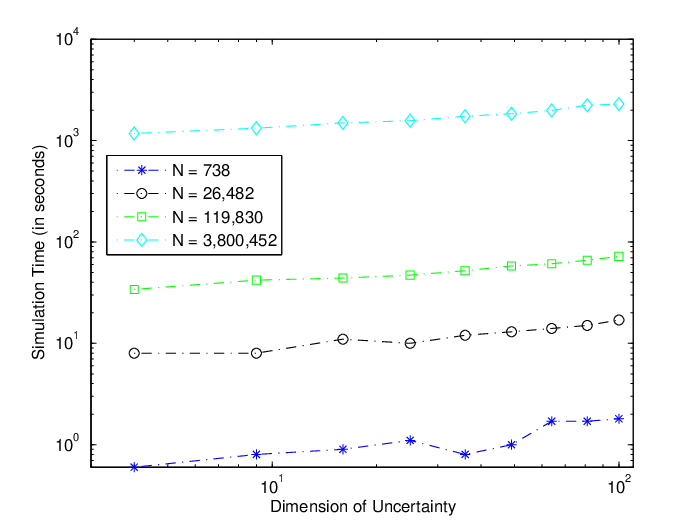
Now we present more extensive numerical experiments for testing the efficiency of our hierarchy sample reuse algorithms. We consider the robust stability of a system of transfer function H⁡(s)=C​(s​I−A)−1​B+DH(s)=C(sI-A)^{-1}B+D with uncertain matrix A=−10​Ik×k+∑ℓ=1dqℓ​ℓ​WA=-10\;I_{k\times k}+\sum_{\ell=1}^{d}q_{\ell}\;\sqrt{\ell}\;W where Ik×kI_{k\times k} is a kk by kk identity matrix, d=k2d=k^{2} is the dimension of uncertainty and WW is a matrix with all elements equal to 11. This is a special case of multiple blocks of real uncertainty. Although this may not be a realistic system, it can be representative for realistic systems in the respect of computational complexity.

When the size of matrix AA increases from 22 to 1010, the dimension of uncertainty increases from 44 to 100100. The robustness functions for the case that AA is of size 10×1010\times 10 is shown in Figure 14. The computing time is shown in Figure 15 for various problem sizes. The sample size is chosen by the Chernoff bound N=⌈ln⁡2δ2​ε2⌉N=\left\lceil\frac{\ln\frac{2}{\delta}}{2\varepsilon^{2}}\right\rceil as 738, 26482, 119830, 3800452738,\;26482,\;119830,\;3800452 corresponding to ε=δ=0.05, 0.01, 0.005, 0.001\varepsilon=\delta=0.05,\;0.01,\;0.005,\;0.001 respectively.

Refer to caption

Figure 14. Robustness Functions (Dimension d=100d=100. Sample size N=119,830N=119,830.)

Refer to caption

Figure 15. Simulation Time

Traditionally, it is widely believed that the classical deterministic robustness analysis are usually more efficient than randomized algorithms. However, as can be seen from Figure 15, our numerical experiments indicates that, if one is willing to accept our probabilistic robustness measure, the robustness analysis via hierarchy sample reuse algorithms can be generally far more efficient.

8. Conclusion

In this paper, we develop a new statistical approach for robustness analysis which requires an extremely low complexity that is independent of the dimension of uncertainty space. Our proposed robustness measure is less conservative as compared to the existing probabilistic robustness measure. The fundamental connection between our measure and the existing one is also established.

References

  • [1] E. W. BAI, R. TEMPO, AND M. FU, “Worst-case properties of the uniform distribution and randomized algorithms for robustness analysis,” Mathematics of Control, Signals and Systems, vol. 11, pp. 183-196, 1998.
  • [2] B. R. BARMISH AND C. M. LAGOA, “The uniform distribution: a rigorous justification for its use in robustness analysis,” Mathematics of Control, Signals and Systems, vol. 10 (1997), pp. 203-222.
  • [3] B. R. BARMISH, C. M. LAGOA, AND R. TEMPO, “Radially truncated uniform distributions for probabilistic robustness of control systems,” Proc. of American Control Conference, pp. 853-857, Albuquerque, New Mexico, June 1997.
  • [4] B. R. BARMISH AND P. S. SHCHERBAKOV, “On avoiding vertexization of robustness problems: The approximate feasibility concept,” IEEE Transactions on Automatic Control, vol. 42, pp. 819-824, 2002.
  • [5] X. CHEN, K. ZHOU, AND J. ARAVENA, “Fast construction of robustness degradation function,” SIAM Journal on Control and Optimization, vol. 42, pp. 1960-1971, 2004.
  • [6] X. CHEN, K. ZHOU, AND J. ARAVENA, “Fast universal algorithms for robustness analysis,” Proceedings of IEEE Conference on Decision and Control, pp. 1926-1931, Maui, Hawaii, December 2003.
  • [7] X. CHEN, K. ZHOU, AND J. ARAVENA, “Probabilistic robustness analysis — Risks, complexity and algorithms,” submitted for publication.
  • [8] H. CHERNOFF, “A measure of asymptotic efficiency for tests of a hypothesis based on the sum of observations,” Annals of Mathematical Statistics, vol. 23, pp. 493-507, 1952.
  • [9] J. C. DOYLE AND G. STEIN, “Multivariable feedback design: concepts for a classical/modern synthesis,” IEEE Trans. Autom. Control, vol. 26, pp. 4-16, 1981.
  • [10] R. R DE GASTON AND M. G. SAFONOV, “Exact calculation of the multiloop stability margin,” IEEE Trans. Autom. Control, vol. 33, pp. 156-171, 1988.
  • [11] S. KANEV, B. De SCHUTTER, AND M. VERHAEGEN, “An ellipsoid algorithm for probabilistic robust controller design,” Systems and Control Letters, vol. 49, pp. 365-375, 2003.
  • [12] V. KOLTCHINSKII, C.T. ABDALLAH, M. ARIOLA, P. DORATO, AND D. PANCHENKO, “Improved sample complexity estimates for statistical learning control of uncertain systems,” IEEE Transactions on Automatic Control, vol. 46, pp. 2383-2388, 2000.
  • [13] L. QIU, B. BERNHARDSSON, A. RANTZER, E. J. DAVISON, P. M. YOUNG, AND J. C. DOYLE, “A formula for computation of the real stability radius,” vol. 31, pp. 879-890, 1995.
  • [14] R. F. STENGEL AND L. R. RAY, “Stochastic robustness of linear time-invariant systems,” IEEE Transaction on Automatic Control, vol. 36, pp. 82-87, 1991.
  • [15] Q. WANG AND R. F. STENGEL, “Robust control of nonlinear systems with parametric uncertainty,” Automatica, vol. 38, pp. 1591-1599, 2002.
  • [16] K. ZHOU, J. C. DOYLE, AND K. GLOVER, Robust and Optimal Control, Prentice Hall, Upper Saddle River, NJ, 1996.

Appendix A Proof of Theorem 1

The following Lemma 1 is due to [3].

Lemma 1.

For any robustness requirement, inff𝚫∈𝒢Pr⁡{𝕀⁡(𝚫)=1∣‖𝚫‖≤γ}=ℙ¯​(γ)\inf_{f_{\boldsymbol{\varDelta}}\in\mathscr{G}}\Pr\{\mathbb{I}(\boldsymbol{\varDelta})=1\mid||\boldsymbol{\varDelta}||\leq\gamma\}=\underline{\mathbb{P}}(\gamma).

Lemma 2.

𝒢\mathscr{G} is a superset of ℱ\mathscr{F}, i.e., 𝒢⊇ℱ\mathscr{G}\supseteq\mathscr{F}.

Proof.

Let f𝚫∈ℱf_{\boldsymbol{\varDelta}}\in\mathscr{F}. We need to show f𝚫∈𝒢f_{\boldsymbol{\varDelta}}\in\mathscr{G}. Let 0<r1<r20<r_{1}<r_{2} be two numbers such that, for any Δ1,Δ2\varDelta_{1},\;\varDelta_{2} satisfying ‖Δ1‖=r1,‖Δ2‖=r2||\varDelta_{1}||=r_{1},\;||\varDelta_{2}||=r_{2}, both f𝚫​(Δ1)f_{\boldsymbol{\varDelta}}(\varDelta_{1}) and f𝚫​(Δ2)f_{\boldsymbol{\varDelta}}(\varDelta_{2}) exist. By the radial symmetry of the distribution of 𝚫\boldsymbol{\varDelta}, we can write f𝚫​(Δi)f_{\boldsymbol{\varDelta}}(\varDelta_{i}) as g⁡(ri)g(r_{i}) for i=1, 2i=1,\;2. Clearly, the existence implies that g(.)g(.) is continuous at r=ri,i=1,2r=r_{i},\;i=1,2. Let c=∫v∈ℬ1𝑑vc=\int_{v\in\mathcal{B}_{1}}dv. By the radial symmetry of the distribution of 𝚫\boldsymbol{\varDelta} and the scaling property of the function ||.||||.||, we have f‖𝚫‖​(ri)=limε→012​ε​∫ri−εri+εg⁡(ρ)​n​c​ρn−1​𝑑ρf_{||\boldsymbol{\varDelta}||}(r_{i})=\lim_{\varepsilon\to 0}\frac{1}{2\varepsilon}\int_{r_{i}-\varepsilon}^{r_{i}+\varepsilon}g(\rho)\;nc\rho^{n-1}\;d\rho for i=1,2i=1,2, where nn is the dimension of 𝚫\boldsymbol{\varDelta}. Hence, f‖𝚫‖​(r)f_{||\boldsymbol{\varDelta}||}(r) is continuous at r=ri,i=1,2r=r_{i},\;i=1,2. Recall that f𝚫∈ℱf_{\boldsymbol{\varDelta}}\in\mathscr{F}, we have f‖𝚫‖​(r1)≥f‖𝚫‖​(r2)f_{||\boldsymbol{\varDelta}||}(r_{1})\geq f_{||\boldsymbol{\varDelta}||}(r_{2}). On the other hand, by the radial symmetry of the distribution of 𝚫\boldsymbol{\varDelta} and the scaling property of the function ||.||||.||, we have g⁡(ri)=limε↓0∫ri−εri+εf‖𝚫‖​(ρ)​𝑑ρc​(ri+ε)n−c​(ri−ε)ng(r_{i})=\lim_{\varepsilon\downarrow 0}\frac{\int_{r_{i}-\varepsilon}^{r_{i}+\varepsilon}f_{||\boldsymbol{\varDelta}||}(\rho)\;d\rho}{c(r_{i}+\varepsilon)^{n}-c(r_{i}-\varepsilon)^{n}} for i=1,2i=1,2. By the continuity of f‖𝚫‖​(r)f_{||\boldsymbol{\varDelta}||}(r) at rir_{i}, we have g⁡(ri)=f‖𝚫‖​(ri)n​c​rin−1g(r_{i})=\frac{f_{||\boldsymbol{\varDelta}||}(r_{i})}{n\;c\;r_{i}^{n-1}} for i=1,2i=1,2. It follows that g⁡(r1)g⁡(r2)=(r2r1)n−1​f‖𝚫‖​(r1)f‖𝚫‖​(r2)≥(r2r1)n−1≥1\frac{g(r_{1})}{g(r_{2})}=\left(\frac{r_{2}}{r_{1}}\right)^{n-1}\frac{f_{||\boldsymbol{\varDelta}||}(r_{1})}{f_{||\boldsymbol{\varDelta}||}(r_{2})}\geq\left(\frac{r_{2}}{r_{1}}\right)^{n-1}\geq 1, implying that f𝚫∈𝒢f_{\boldsymbol{\varDelta}}\in\mathscr{G}. Hence, 𝒢⊇ℱ\mathscr{G}\supseteq\mathscr{F}.

□\Box

Lemma 3.

For any S⊆∂ℬS\subseteq\partial\mathcal{B}, area⁡(Sr)=rn−1​area​(S)\mathrm{area}(S_{r})=r^{n-1}\;\mathrm{area}(S) where Sr={r​Δ:Δ∈S}S_{r}=\{r\varDelta:\;\varDelta\in S\} and nn is the dimension of ℬ\mathcal{B}.

Proof.

By the scalable property of ||.||||.||,

{ρrΔ:r−ε1<ρ<r+ε2,Δ∈Sr}\displaystyle\left\{\frac{\rho}{r}\varDelta:r-\varepsilon_{1}<\rho<r+\varepsilon_{2},\;\varDelta\in S_{r}\right\} =\displaystyle= {ρΔ:r−ε1<ρ<r+ε2,Δ∈S}={Δ:r−ε1<ρ<r+ε2,Δρ∈S}.\displaystyle\left\{\rho\varDelta:r-\varepsilon_{1}<\rho<r+\varepsilon_{2},\;\varDelta\in S\right\}=\left\{\varDelta:r-\varepsilon_{1}<\rho<r+\varepsilon_{2},\;\frac{\varDelta}{\rho}\in S\right\}.

Hence, by invoking the definition (1.1), area(Sr)=limε1↓0ε2↓0∫q∈{Δ:r−ε1<ρ<r+ε2,Δρ∈S}dqε1+ε2\mathrm{area}(S_{r})=\lim_{\varepsilon_{1}\downarrow 0\atop{\varepsilon_{2}\downarrow 0}}\frac{\int_{q\in\left\{\varDelta:\;r-\varepsilon_{1}<\rho<r+\varepsilon_{2},\;\frac{\varDelta}{\rho}\in S\right\}}dq}{\varepsilon_{1}+\varepsilon_{2}}. Making a change of variable q=r​q′q=rq^{\prime} yields

area⁡(Sr)\displaystyle\mathrm{area}(S_{r}) =\displaystyle= rnlimε1↓0ε2↓0∫q′∈{Δ:r−ε1<ρ<r+ε2,r​Δρ∈S}dq′ε1+ε2\displaystyle r^{n}\lim_{\varepsilon_{1}\downarrow 0\atop{\varepsilon_{2}\downarrow 0}}\frac{\int_{q^{\prime}\in\left\{\varDelta:\;r-\varepsilon_{1}<\rho<r+\varepsilon_{2},\;\frac{r\varDelta}{\rho}\in S\right\}}dq^{\prime}}{\varepsilon_{1}+\varepsilon_{2}}
=\displaystyle= rn−1limε1↓0ε2↓0∫q′∈{ρrΔ:−ε1r≤ρr−1≤ε2r,Δ∈S}dq′(ε1+ε2)/r\displaystyle r^{n-1}\lim_{\varepsilon_{1}\downarrow 0\atop{\varepsilon_{2}\downarrow 0}}\frac{\int_{q^{\prime}\in\left\{\frac{\rho}{r}\varDelta:\;-\frac{\varepsilon_{1}}{r}\leq\frac{\rho}{r}-1\leq\frac{\varepsilon_{2}}{r},\;\varDelta\in S\right\}}dq^{\prime}}{(\varepsilon_{1}+\varepsilon_{2})/\penalty r}
=\displaystyle= rn−1limε1↓0ε2↓0∫q′∈{ρΔ:−ε1≤ρ−1≤ε2,Δ∈S}dq′ε1+ε2\displaystyle r^{n-1}\lim_{\varepsilon_{1}\downarrow 0\atop{\varepsilon_{2}\downarrow 0}}\frac{\int_{q^{\prime}\in\left\{\rho\varDelta:\;-\varepsilon_{1}\leq\rho-1\leq\varepsilon_{2},\;\varDelta\in S\right\}}dq^{\prime}}{\varepsilon_{1}+\varepsilon_{2}}
=\displaystyle= rn−1​area​(S).\displaystyle r^{n-1}\mathrm{area}(S).

□\Box

Lemma 4.

Suppose the distribution of 𝚫\boldsymbol{\varDelta} is radially symmetrical. Let SS be a subset of ∂ℬ={Δ:‖Δ‖=1}\partial\mathcal{B}=\{\varDelta:||\varDelta||=1\}. Then, Pr{𝚫‖𝚫‖∈S|||𝚫||=ρ}=area⁡(S)area⁡(∂ℬ)\Pr\left\{\left.\frac{\boldsymbol{\varDelta}}{||\boldsymbol{\varDelta}||}\in S\;\right|\;||\boldsymbol{\varDelta}||=\rho\right\}=\frac{\mathrm{area}(S)}{\mathrm{area}(\partial\mathcal{B})} for any ρ>0\rho>0 such that f‖𝚫‖​(ρ)f_{||\boldsymbol{\varDelta}||}(\rho) is continuous.

Proof.

By the definition of the conditional probability,

Pr{𝚫‖𝚫‖∈S|||𝚫||=ρ}=limε1↓0ε2↓0Pr{𝚫‖𝚫‖∈S,ρ−ε1≤||𝚫||≤ρ+ε2}Pr{ρ−ε1≤||𝚫||≤ρ+ε2}.\Pr\left\{\left.\frac{\boldsymbol{\varDelta}}{||\boldsymbol{\varDelta}||}\in S\;\right|\;||\boldsymbol{\varDelta}||=\rho\right\}=\lim_{\varepsilon_{1}\downarrow 0\atop{\varepsilon_{2}\downarrow 0}}\frac{\Pr\left\{\frac{\boldsymbol{\varDelta}}{||\boldsymbol{\varDelta}||}\in S,\;\rho-\varepsilon_{1}\leq||\boldsymbol{\varDelta}||\leq\rho+\varepsilon_{2}\right\}}{\Pr\left\{\rho-\varepsilon_{1}\leq||\boldsymbol{\varDelta}||\leq\rho+\varepsilon_{2}\right\}}.

We claim that {𝚫‖𝚫‖∈S,ρ−ε1≤||𝚫||≤ρ+ε2}={𝚫∈Sρ,ε1,ε2}\left\{\frac{\boldsymbol{\varDelta}}{||\boldsymbol{\varDelta}||}\in S,\;\rho-\varepsilon_{1}\leq||\boldsymbol{\varDelta}||\leq\rho+\varepsilon_{2}\right\}=\{\boldsymbol{\varDelta}\in S_{\rho,\varepsilon_{1},\varepsilon_{2}}\} where Sρ,ε1,ε2={Δ:Δρ′∈S,ρ−ε1≤ρ′≤ρ+ε2}S_{\rho,\varepsilon_{1},\varepsilon_{2}}=\{\varDelta:\frac{\varDelta}{\rho^{\prime}}\in S,\;\rho-\varepsilon_{1}\leq\rho^{\prime}\leq\rho+\varepsilon_{2}\}. To show this claim, it suffices to show that {Δ:Δ‖Δ‖∈S,ρ−ε1≤||Δ||≤ρ+ε2}=Sρ,ε1,ε2\left\{\varDelta:\frac{\varDelta}{||\varDelta||}\in S,\;\rho-\varepsilon_{1}\leq||\varDelta||\leq\rho+\varepsilon_{2}\right\}=S_{\rho,\varepsilon_{1},\varepsilon_{2}}. Let Δ∈Sρ,ε1,ε2\varDelta\in S_{\rho,\varepsilon_{1},\varepsilon_{2}}. By definition, there exists ρ′∈[ρ−ε1,ρ+ε2]\rho^{\prime}\in[\rho-\varepsilon_{1},\rho+\varepsilon_{2}] such that Δρ′∈S\frac{\varDelta}{\rho^{\prime}}\in S. Therefore, by the scalable property of the function ||.||||.||, we have ‖Δ‖=||ρ′​Δρ′||=ρ′​||Δρ′||=ρ′∈[ρ−ε1,ρ+ε2]||\varDelta||=\left|\left|\rho^{\prime}\frac{\varDelta}{\rho^{\prime}}\right|\right|=\rho^{\prime}\left|\left|\frac{\varDelta}{\rho^{\prime}}\right|\right|=\rho^{\prime}\in[\rho-\varepsilon_{1},\rho+\varepsilon_{2}] and Δ‖Δ‖=Δρ′‖Δ‖ρ′=Δρ′||Δρ′||=Δρ′∈S\frac{\varDelta}{||\varDelta||}=\frac{\frac{\varDelta}{\rho^{\prime}}}{\frac{||\varDelta||}{\rho^{\prime}}}=\frac{\frac{\varDelta}{\rho^{\prime}}}{\left|\left|\frac{\varDelta}{\rho^{\prime}}\right|\right|}=\frac{\varDelta}{\rho^{\prime}}\in S. This implies that Δ∈{Δ:Δ‖Δ‖∈S,ρ−ε1≤||Δ||≤ρ+ε2}\varDelta\in\left\{\varDelta:\frac{\varDelta}{||\varDelta||}\in S,\;\rho-\varepsilon_{1}\leq||\varDelta||\leq\rho+\varepsilon_{2}\right\}.

Now let Δ∈{Δ:Δ‖Δ‖∈S,ρ−ε1≤||Δ||≤ρ+ε2}\varDelta\in\left\{\varDelta:\frac{\varDelta}{||\varDelta||}\in S,\;\rho-\varepsilon_{1}\leq||\varDelta||\leq\rho+\varepsilon_{2}\right\} and ρ′=‖Δ‖\rho^{\prime}=||\varDelta||. By definition, ρ−ε1≤ρ′≤ρ+ε2,Δρ′∈S\rho-\varepsilon_{1}\leq\rho^{\prime}\leq\rho+\varepsilon_{2},\;\frac{\varDelta}{\rho^{\prime}}\in S. Hence, Δ∈Sρ,ε1,ε2\varDelta\in S_{\rho,\varepsilon_{1},\varepsilon_{2}}. The claim is thus proved and we have

Pr{𝚫‖𝚫‖∈S,ρ−ε1≤||𝚫||≤ρ+ε2}=Pr{𝚫∈Sρ,ε1,ε2}.\Pr\left\{\frac{\boldsymbol{\varDelta}}{||\boldsymbol{\varDelta}||}\in S,\;\rho-\varepsilon_{1}\leq||\boldsymbol{\varDelta}||\leq\rho+\varepsilon_{2}\right\}=\Pr\{\boldsymbol{\varDelta}\in S_{\rho,\varepsilon_{1},\varepsilon_{2}}\}.

Let Sρ′={ρ′​Δ:Δ∈S}S_{\rho^{\prime}}=\{\rho^{\prime}\varDelta:\varDelta\in S\}. Then, Sρ′⊆∂ℬρ′S_{\rho^{\prime}}\subseteq\partial\mathcal{B}_{\rho^{\prime}} and Sρ,ε1,ε2={Δ:Δ∈Sρ′,ρ−ε1≤ρ′≤ρ+ε2}S_{\rho,\varepsilon_{1},\varepsilon_{2}}=\{\varDelta:\varDelta\in S_{\rho^{\prime}},\rho-\varepsilon_{1}\leq\rho^{\prime}\leq\rho+\varepsilon_{2}\}. By the notion of the radially symmetrical distribution of 𝚫\boldsymbol{\varDelta} and the property of the area function shown in Lemma 3, we have Pr⁡{𝚫∈Sρ′∣‖𝚫‖=ρ′}=area⁡(Sρ′)area⁡(∂ℬρ′)=ρ′n−1​area​(S)ρ′n−1​area​(∂ℬ)=area⁡(S)area⁡(∂ℬ)\Pr\{\boldsymbol{\varDelta}\in S_{\rho^{\prime}}\mid||\boldsymbol{\varDelta}||=\rho^{\prime}\}=\frac{\mathrm{area}(S_{\rho^{\prime}})}{\mathrm{area}(\partial\mathcal{B}_{\rho^{\prime}})}=\frac{{\rho^{\prime}}^{n-1}\mathrm{area}(S)}{{\rho^{\prime}}^{n-1}\mathrm{area}(\partial\mathcal{B})}=\frac{\mathrm{area}(S)}{\mathrm{area}(\partial\mathcal{B})}. On the other hand, by the definition of the conditional probability,

Pr⁡{𝚫∈Sρ′∣‖𝚫‖=ρ′}=limε1↓0ε2↓0Pr{𝚫∈Sρ,ε1,ε2}Pr{ρ−ε1≤||𝚫||≤ρ+ε2}.\Pr\{\boldsymbol{\varDelta}\in S_{\rho^{\prime}}\mid||\boldsymbol{\varDelta}||=\rho^{\prime}\}=\lim_{\varepsilon_{1}\downarrow 0\atop{\varepsilon_{2}\downarrow 0}}\frac{\Pr\{\boldsymbol{\varDelta}\in S_{\rho,\varepsilon_{1},\varepsilon_{2}}\}}{\Pr\left\{\rho-\varepsilon_{1}\leq||\boldsymbol{\varDelta}||\leq\rho+\varepsilon_{2}\right\}}.

It follows that Pr{𝚫‖𝚫‖∈S|||𝚫||=ρ}=limε1↓0ε2↓0Pr{𝚫∈Sρ,ε1,ε2}Pr{ρ−ε1≤||𝚫||≤ρ+ε2}=area⁡(S)area⁡(∂ℬ)\Pr\left\{\left.\frac{\boldsymbol{\varDelta}}{||\boldsymbol{\varDelta}||}\in S\;\right|\;||\boldsymbol{\varDelta}||=\rho\right\}=\lim_{\varepsilon_{1}\downarrow 0\atop{\varepsilon_{2}\downarrow 0}}\frac{\Pr\{\boldsymbol{\varDelta}\in S_{\rho,\varepsilon_{1},\varepsilon_{2}}\}}{\Pr\left\{\rho-\varepsilon_{1}\leq||\boldsymbol{\varDelta}||\leq\rho+\varepsilon_{2}\right\}}=\frac{\mathrm{area}(S)}{\mathrm{area}(\partial\mathcal{B})}.

□\Box

Lemma 5.

Suppose f‖𝚫‖(.)f_{||\boldsymbol{\varDelta}||}(.) is continuous in (a,b)(a,b). Then, Pr⁡{𝚫‖𝚫‖∈S∣a<‖𝚫‖<b}=area⁡(S)area⁡(∂ℬ)\Pr\left\{\frac{\boldsymbol{\varDelta}}{||\boldsymbol{\varDelta}||}\in S\mid a<||\boldsymbol{\varDelta}||<b\right\}=\frac{\mathrm{area}(S)}{\mathrm{area}(\partial\mathcal{B})}.

Proof.

Let η>0\eta>0 and δ∈(0,b−a2)\delta\in\left(0,\frac{b-a}{2}\right). For notational simplicity, let c=area⁡(S)area⁡(∂ℬ)c=\frac{\mathrm{area}(S)}{\mathrm{area}(\partial\mathcal{B})}. By Lemma 4, for any ρ∈[a+δ,b−δ]\rho\in[a+\delta,b-\delta], we can find ε=ε⁡(ρ)\varepsilon=\varepsilon(\rho) such that |Pr⁡{𝚫‖𝚫‖∈S∣ρ−ε1≤‖𝚫‖≤ρ+ε2}−c|<η\left|\Pr\left\{\frac{\boldsymbol{\varDelta}}{||\boldsymbol{\varDelta}||}\in S\mid\rho-\varepsilon_{1}\leq||\boldsymbol{\varDelta}||\leq\rho+\varepsilon_{2}\right\}-c\right|<\eta for any positive ε1,ε2\varepsilon_{1},\varepsilon_{2} less than ε⁡(ρ)\varepsilon(\rho). Hence, the union of the open intervals ∪ρ∈[a+δ,b−δ](ρ−ε(ρ),ρ+ε(ρ))\cup_{\rho\in[a+\delta,b-\delta]}(\rho-\varepsilon(\rho),\rho+\varepsilon(\rho)) will cover interval [a+δ,b−δ][a+\delta,b-\delta]. By the finite coverage theorem, we can choose finite number of ρi\rho_{i} from [a+δ,b−δ][a+\delta,b-\delta] such that ∪i=1k(ρi−ε(ρi),ρi+ε(ρi))\cup_{i=1}^{k}(\rho_{i}-\varepsilon(\rho_{i}),\rho_{i}+\varepsilon(\rho_{i})) covers interval [a+δ,b−δ][a+\delta,b-\delta] and that none of (ρi−ε⁡(ρi),ρi+ε⁡(ρi))(\rho_{i}-\varepsilon(\rho_{i}),\rho_{i}+\varepsilon(\rho_{i})) is nested in another. By using the mid-points of the intersections of every two consecutive intervals as dividing points, we can partition [a+δ,b−δ][a+\delta,b-\delta] as kk intervals [ai,bi][a_{i},b_{i}] such that |Pr⁡{𝚫‖𝚫‖∈S∣ai≤‖𝚫‖≤bi}−c|<η\left|\Pr\left\{\frac{\boldsymbol{\varDelta}}{||\boldsymbol{\varDelta}||}\in S\mid a_{i}\leq||\boldsymbol{\varDelta}||\leq b_{i}\right\}-c\right|<\eta for i=1,⋯,ki=1,\cdots,k. Therefore, |Pr{𝚫‖𝚫‖∈S,ai≤||𝚫||≤bi}−cPr{ai≤||𝚫||≤bi}|<ηPr{ai≤||𝚫||≤bi}\left|\Pr\left\{\frac{\boldsymbol{\varDelta}}{||\boldsymbol{\varDelta}||}\in S,\;a_{i}\leq||\boldsymbol{\varDelta}||\leq b_{i}\right\}-c\Pr\left\{a_{i}\leq||\boldsymbol{\varDelta}||\leq b_{i}\right\}\right|<\eta\Pr\left\{a_{i}\leq||\boldsymbol{\varDelta}||\leq b_{i}\right\} for i=1,⋯,ki=1,\cdots,k and

|∑i=1k[Pr{𝚫‖𝚫‖∈S,ai≤||𝚫||≤bi}−cPr{ai≤||𝚫||≤bi}]|<η∑i=1kPr{ai≤||𝚫||≤bi}.\left|\sum_{i=1}^{k}\left[\Pr\left\{\frac{\boldsymbol{\varDelta}}{||\boldsymbol{\varDelta}||}\in S,\;a_{i}\leq||\boldsymbol{\varDelta}||\leq b_{i}\right\}-c\Pr\left\{a_{i}\leq||\boldsymbol{\varDelta}||\leq b_{i}\right\}\right]\right|<\eta\sum_{i=1}^{k}\Pr\left\{a_{i}\leq||\boldsymbol{\varDelta}||\leq b_{i}\right\}.

That is, |Pr{𝚫‖𝚫‖∈S,a+δ≤||𝚫||≤b−δ}−cPr{a+δ≤||𝚫||≤b−δ}|<ηPr{a+δ≤||𝚫||≤b−δ}\left|\Pr\left\{\frac{\boldsymbol{\varDelta}}{||\boldsymbol{\varDelta}||}\in S,\;a+\delta\leq||\boldsymbol{\varDelta}||\leq b-\delta\right\}-c\Pr\left\{a+\delta\leq||\boldsymbol{\varDelta}||\leq b-\delta\right\}\right|<\eta\Pr\left\{a+\delta\leq||\boldsymbol{\varDelta}||\leq b-\delta\right\}. As a result, |Pr⁡{𝚫‖𝚫‖∈S∣a+δ≤‖𝚫‖≤b−δ}−c|<η\left|\Pr\left\{\frac{\boldsymbol{\varDelta}}{||\boldsymbol{\varDelta}||}\in S\mid a+\delta\leq||\boldsymbol{\varDelta}||\leq b-\delta\right\}-c\right|<\eta. Since η\eta can be arbitrarily small, we have

Pr{𝚫‖𝚫‖∈S,a+δ≤||𝚫||≤b−δ}=cPr{a+δ≤||𝚫||≤b−δ}.\Pr\left\{\frac{\boldsymbol{\varDelta}}{||\boldsymbol{\varDelta}||}\in S,\;a+\delta\leq||\boldsymbol{\varDelta}||\leq b-\delta\right\}=c\Pr\left\{a+\delta\leq||\boldsymbol{\varDelta}||\leq b-\delta\right\}.

By the assumption that f‖𝚫‖(.)f_{||\boldsymbol{\varDelta}||}(.) is piece-wise continuous, we have Pr{ρ≤||𝚫||≤ρ+δ}→0\Pr\left\{\rho\leq||\boldsymbol{\varDelta}||\leq\rho+\delta\right\}\to 0 as δ↓0\delta\downarrow 0 for all ρ≥0\rho\geq 0. Hence,

limδ↓0|Pr{𝚫‖𝚫‖∈S,a+δ≤||𝚫||≤b−δ}−Pr{𝚫‖𝚫‖∈S,a<||𝚫||<b}|\displaystyle\lim_{\delta\downarrow 0}\left|\Pr\left\{\frac{\boldsymbol{\varDelta}}{||\boldsymbol{\varDelta}||}\in S,\;a+\delta\leq||\boldsymbol{\varDelta}||\leq b-\delta\right\}-\Pr\left\{\frac{\boldsymbol{\varDelta}}{||\boldsymbol{\varDelta}||}\in S,\;a<||\boldsymbol{\varDelta}||<b\right\}\right|
=\displaystyle= limδ↓0[Pr{𝚫‖𝚫‖∈S,a<||𝚫||<a+δ}+Pr{𝚫‖𝚫‖∈S,b−δ<||𝚫||<b}]\displaystyle\lim_{\delta\downarrow 0}\left[\Pr\left\{\frac{\boldsymbol{\varDelta}}{||\boldsymbol{\varDelta}||}\in S,\;a<||\boldsymbol{\varDelta}||<a+\delta\right\}+\Pr\left\{\frac{\boldsymbol{\varDelta}}{||\boldsymbol{\varDelta}||}\in S,\;b-\delta<||\boldsymbol{\varDelta}||<b\right\}\right]
≤\displaystyle\leq limδ↓0[Pr{a<||𝚫||<a+δ}+Pr{b−δ<||𝚫||<b}]=0,\displaystyle\lim_{\delta\downarrow 0}\left[\Pr\left\{a<||\boldsymbol{\varDelta}||<a+\delta\right\}+\Pr\left\{b-\delta<||\boldsymbol{\varDelta}||<b\right\}\right]=0,

and so limδ↓0Pr{𝚫‖𝚫‖∈S,a+δ≤||𝚫||≤b−δ}=Pr{𝚫‖𝚫‖∈S,a<||𝚫||<b}\lim_{\delta\downarrow 0}\Pr\left\{\frac{\boldsymbol{\varDelta}}{||\boldsymbol{\varDelta}||}\in S,\;a+\delta\leq||\boldsymbol{\varDelta}||\leq b-\delta\right\}=\Pr\left\{\frac{\boldsymbol{\varDelta}}{||\boldsymbol{\varDelta}||}\in S,\;a<||\boldsymbol{\varDelta}||<b\right\}. Similarly,

limδ↓0|Pr{a+δ≤||𝚫||≤b−δ}−Pr{a<||𝚫||<b}|\displaystyle\lim_{\delta\downarrow 0}\left|\Pr\left\{a+\delta\leq||\boldsymbol{\varDelta}||\leq b-\delta\right\}-\Pr\left\{a<||\boldsymbol{\varDelta}||<b\right\}\right|
=\displaystyle= limδ↓0[Pr{a<||𝚫||<a+δ}+Pr{b−δ<||𝚫||<b}]=0,\displaystyle\lim_{\delta\downarrow 0}\left[\Pr\left\{a<||\boldsymbol{\varDelta}||<a+\delta\right\}+\Pr\left\{b-\delta<||\boldsymbol{\varDelta}||<b\right\}\right]=0,

and so limδ↓0Pr{a+δ≤||𝚫||≤b−δ}=Pr{a<||𝚫||<b}\lim_{\delta\downarrow 0}\Pr\left\{a+\delta\leq||\boldsymbol{\varDelta}||\leq b-\delta\right\}=\Pr\left\{a<||\boldsymbol{\varDelta}||<b\right\}. It follows that

Pr{𝚫‖𝚫‖∈S,a<||𝚫||<b}=cPr{a<||𝚫||<b}.\Pr\left\{\frac{\boldsymbol{\varDelta}}{||\boldsymbol{\varDelta}||}\in S,\;a<||\boldsymbol{\varDelta}||<b\right\}=c\Pr\left\{a<||\boldsymbol{\varDelta}||<b\right\}.

This completes the proof.

□\Box

Lemma 6.

Suppose that the distribution of 𝚫\boldsymbol{\varDelta} is radially symmetrical and that f‖𝚫‖(.)f_{||\boldsymbol{\varDelta}||}(.) is piece-wise continuous over (0,∞)(0,\infty). Then, 𝚫‖𝚫‖\frac{\boldsymbol{\varDelta}}{||\boldsymbol{\varDelta}||} is independent with ‖𝚫‖||\boldsymbol{\varDelta}||. Moreover, 𝚫‖𝚫‖\frac{\boldsymbol{\varDelta}}{||\boldsymbol{\varDelta}||} is uniformly distributed over {Δ:‖Δ‖=1}\{\varDelta:||\varDelta||=1\}.

Proof.

Since f‖𝚫‖(.)f_{||\boldsymbol{\varDelta}||}(.) is piece-wise continuous over (0,∞)(0,\infty), we can represent (0,∞)(0,\infty) as a union of open intervals (ai,bi)(a_{i},b_{i}) where f‖𝚫‖(.)f_{||\boldsymbol{\varDelta}||}(.) is continuous and the set of discrete values ρj,j=1,2,⋯\rho_{j},\;j=1,2,\cdots for which f‖𝚫‖(.)f_{||\boldsymbol{\varDelta}||}(.) is discontinuous. We can enumerate the intervals and the discrete values such that bi−aib_{i}-a_{i} is non-increasing with respect to ii and that ρj−ρj−1\rho_{j}-\rho_{j-1} is non-increasing with respect to jj. Then, Pr{𝚫‖𝚫‖∈S,||𝚫||=ρj}=0,j=1,2,⋯\Pr\left\{\frac{\boldsymbol{\varDelta}}{||\boldsymbol{\varDelta}||}\in S,\;||\boldsymbol{\varDelta}||=\rho_{j}\right\}=0,\;j=1,2,\cdots and, by Lemma 5,

Pr{𝚫‖𝚫‖∈S}\displaystyle\Pr\left\{\frac{\boldsymbol{\varDelta}}{||\boldsymbol{\varDelta}||}\in S\right\} =\displaystyle= ∑iPr{𝚫‖𝚫‖∈S,ai<||𝚫||<bi}+∑jPr{𝚫‖𝚫‖∈S,||𝚫||=ρj}\displaystyle\sum_{i}\Pr\left\{\frac{\boldsymbol{\varDelta}}{||\boldsymbol{\varDelta}||}\in S,\;a_{i}<||\boldsymbol{\varDelta}||<b_{i}\right\}+\sum_{j}\Pr\left\{\frac{\boldsymbol{\varDelta}}{||\boldsymbol{\varDelta}||}\in S,\;||\boldsymbol{\varDelta}||=\rho_{j}\right\}
=\displaystyle= area⁡(S)area⁡(∂ℬ)[∑iPr{ai<||𝚫||<bi}+∑jPr{||𝚫||=ρj}]=area⁡(S)area⁡(∂ℬ).\displaystyle\frac{\mathrm{area}(S)}{\mathrm{area}(\partial\mathcal{B})}\left[\sum_{i}\Pr\left\{a_{i}<||\boldsymbol{\varDelta}||<b_{i}\right\}+\sum_{j}\Pr\left\{||\boldsymbol{\varDelta}||=\rho_{j}\right\}\right]=\frac{\mathrm{area}(S)}{\mathrm{area}(\partial\mathcal{B})}.

Therefore, invoking Lemma 4, we have Pr{𝚫‖𝚫‖∈S∣||𝚫||=ρ}=Pr{𝚫‖𝚫‖∈S}\Pr\left\{\frac{\boldsymbol{\varDelta}}{||\boldsymbol{\varDelta}||}\in S\mid||\boldsymbol{\varDelta}||=\rho\right\}=\Pr\left\{\frac{\boldsymbol{\varDelta}}{||\boldsymbol{\varDelta}||}\in S\right\} for any ρ\rho such that f‖𝚫‖(.)f_{||\boldsymbol{\varDelta}||}(.) is continuous. This implies the independence between 𝚫‖𝚫‖\frac{\boldsymbol{\varDelta}}{||\boldsymbol{\varDelta}||} and ‖𝚫‖||\boldsymbol{\varDelta}||. Moreover, since the argument holds for any S⊆{Δ:‖Δ‖=1}S\subseteq\{\varDelta:||\varDelta||=1\}, we have that 𝚫‖𝚫‖\frac{\boldsymbol{\varDelta}}{||\boldsymbol{\varDelta}||} is uniformly distributed over {Δ:‖Δ‖=1}\{\varDelta:||\varDelta||=1\}. The proof is thus completed.

□\Box

Lemma 7.

Suppose that ϕ(.)\phi(.) is continuous over (a,b)(a,b) and that the distribution of uncertainty 𝚫\boldsymbol{\varDelta} is radially symmetrical and continuous over (a,b)(a,b). Then Pr{𝕀(𝚫)=1,a<||𝚫||<b}=∫abϕ(r)fR(r)dr\Pr\{\mathbb{I}(\boldsymbol{\varDelta})=1,\;a<||\boldsymbol{\varDelta}||<b\}=\int_{a}^{b}\phi(r)f_{R}(r)dr.

Proof.

Define U=𝚫‖𝚫‖,R=‖𝚫‖U=\frac{\boldsymbol{\varDelta}}{||\boldsymbol{\varDelta}||},\;R=||\boldsymbol{\varDelta}|| and fR​(ρ)=d[Pr{R≤ρ}]d​ρf_{R}(\rho)=\frac{d\left[\Pr\{R\leq\rho\}\right]}{d\rho}. By Lemma 6, we have that UU and RR are independent and that UU is uniform over ∂ℬ\partial\mathcal{B}. Hence, the probability density function of U​RUR is 1area⁡(∂ℬ)×fR​(r)\frac{1}{\mathrm{area}(\partial\mathcal{B})}\times f_{R}(r) and, by the Fubini’s Theorem,

Pr{𝕀(𝚫)=1,a<||𝚫||<b}\displaystyle\Pr\{\mathbb{I}(\boldsymbol{\varDelta})=1,\;a<||\boldsymbol{\varDelta}||<b\} =\displaystyle= Pr{𝕀(UR)=1,a<R<b}\displaystyle\Pr\{\mathbb{I}(UR)=1,\;a<R<b\}
=\displaystyle= ∫r=ab∫{u:𝕀(ru)=1,u∈∂ℬ}1area⁡(∂ℬ)fR(r)dudr\displaystyle\int_{r=a}^{b}\int_{\{u:\;\mathbb{I}(ru)=1,\;u\in\partial\mathcal{B}\}}\frac{1}{\mathrm{area}(\partial\mathcal{B})}f_{R}(r)\;dudr
=\displaystyle= ∫r=ab[∫{u:𝕀(ru)=1,u∈∂ℬ}1area⁡(∂ℬ)du]fR(r)dr\displaystyle\int_{r=a}^{b}\left[\int_{\{u:\;\mathbb{I}(ru)=1,\;u\in\partial\mathcal{B}\}}\frac{1}{\mathrm{area}(\partial\mathcal{B})}du\right]f_{R}(r)dr
=\displaystyle= ∫r=abϕ⁡(r)​fR​(r)​𝑑r\displaystyle\int_{r=a}^{b}\phi(r)f_{R}(r)dr

where the last equality follows from the definition of ϕ(.)\phi(.).

□\Box

Lemma 8.

Suppose that ϕ(.)\phi(.) is piece-wise continuous and that f‖𝚫‖(.)f_{||\boldsymbol{\varDelta}||}(.) is piece-wise continuous and non-increasing. Then, Pr⁡{𝕀⁡(𝚫)=1,‖𝚫‖≤γ}=∫0γϕ⁡(ρ)​f‖𝚫‖​(ρ)​𝑑ρ\Pr\{\mathbb{I}(\boldsymbol{\varDelta})=1,\;||\boldsymbol{\varDelta}||\leq\gamma\}=\int_{0}^{\gamma}\phi(\rho)\;f_{||\boldsymbol{\varDelta}||}(\rho)d\rho.

Proof.

Let ε>0\varepsilon>0. Since f‖𝚫‖​(ρ)f_{||\boldsymbol{\varDelta}||}(\rho) is non-increasing, we have f‖𝚫‖​(ρ)≤Pr{||𝚫||≤ε}εf_{||\boldsymbol{\varDelta}||}(\rho)\leq\frac{\Pr\{||\boldsymbol{\varDelta}||\leq\varepsilon\}}{\varepsilon} for ρ∈[ε,ρ]\rho\in[\varepsilon,\rho]. It follows that ϕ⁡(ρ)​f‖𝚫‖​(ρ)\phi(\rho)\;f_{||\boldsymbol{\varDelta}||}(\rho) is piece-wise continuous and bounded for ρ∈[ε,ρ]\rho\in[\varepsilon,\rho]. Hence, the Riemann integral ∫εγϕ⁡(ρ)​f‖𝚫‖​(ρ)​𝑑ρ\int_{\varepsilon}^{\gamma}\phi(\rho)\;f_{||\boldsymbol{\varDelta}||}(\rho)d\rho exists. Note that ∫εγϕ⁡(ρ)​f‖𝚫‖​(ρ)​𝑑ρ≤∫εγf‖𝚫‖​(ρ)​𝑑ρ≤1\int_{\varepsilon}^{\gamma}\phi(\rho)\;f_{||\boldsymbol{\varDelta}||}(\rho)d\rho\leq\int_{\varepsilon}^{\gamma}f_{||\boldsymbol{\varDelta}||}(\rho)d\rho\leq 1 and that ∫εγϕ⁡(ρ)​f‖𝚫‖​(ρ)​𝑑ρ\int_{\varepsilon}^{\gamma}\phi(\rho)\;f_{||\boldsymbol{\varDelta}||}(\rho)d\rho is non-increasing with respect to ε\varepsilon. Thus, limε↓0∫εγϕ⁡(ρ)​f‖𝚫‖​(ρ)​𝑑ρ\lim_{\varepsilon\downarrow 0}\int_{\varepsilon}^{\gamma}\phi(\rho)\;f_{||\boldsymbol{\varDelta}||}(\rho)d\rho exists. This limit is denoted as ∫0γϕ⁡(ρ)​f‖𝚫‖​(ρ)​𝑑ρ\int_{0}^{\gamma}\phi(\rho)\;f_{||\boldsymbol{\varDelta}||}(\rho)d\rho.

Note that we can partition interval (0,γ)(0,\gamma) as a sequence of intervals (ai,bi),i=1,⋯,∞(a_{i},b_{i}),\;i=1,\cdots,\infty such that ai,bi,i=1,2,⋯a_{i},\;b_{i},\;i=1,2,\cdots are discontinuities of f‖𝚫‖​(ρ)f_{||\boldsymbol{\varDelta}||}(\rho) and that bi−aib_{i}-a_{i} is non-increasing with respect to ii. To ensure that the partition is unique, we can handle the situation that some intervals have the same length by enforcing the following criterion: if bi−ai=bj−aj,i<jb_{i}-a_{i}=b_{j}-a_{j},\;i<j then ai<aja_{i}<a_{j}. Then, by the property of the Riemann integral, we have ∫0γϕ⁡(ρ)​f‖𝚫‖​(ρ)​𝑑ρ=∑i=1∞∫aibiϕ⁡(ρ)​f‖𝚫‖​(ρ)​𝑑ρ\int_{0}^{\gamma}\phi(\rho)\;f_{||\boldsymbol{\varDelta}||}(\rho)d\rho=\sum_{i=1}^{\infty}\int_{a_{i}}^{b_{i}}\phi(\rho)\;f_{||\boldsymbol{\varDelta}||}(\rho)d\rho. On the other hand, since Pr{||𝚫||=ai}=Pr{||𝚫||=bi}=0\Pr\{||\boldsymbol{\varDelta}||=a_{i}\}=\Pr\{||\boldsymbol{\varDelta}||=b_{i}\}=0 for i=1,2⋯,∞i=1,2\cdots,\infty, we have

(A.1) Pr⁡{𝕀⁡(𝚫)=1,‖𝚫‖≤γ}\displaystyle\Pr\{\mathbb{I}(\boldsymbol{\varDelta})=1,\;||\boldsymbol{\varDelta}||\leq\gamma\} =\displaystyle= ∑i=1∞Pr{𝕀(𝚫)=1,ai<||𝚫||<bi}\displaystyle\sum_{i=1}^{\infty}\Pr\{\mathbb{I}(\boldsymbol{\varDelta})=1,\;a_{i}<||\boldsymbol{\varDelta}||<b_{i}\}
=\displaystyle= ∑i=1∞∫aibiϕ⁡(ρ)​f‖𝚫‖​(ρ)​𝑑ρ\displaystyle\sum_{i=1}^{\infty}\int_{a_{i}}^{b_{i}}\phi(\rho)\;f_{||\boldsymbol{\varDelta}||}(\rho)d\rho
=\displaystyle= ∫0γϕ⁡(ρ)​f‖𝚫‖​(ρ)​𝑑ρ\displaystyle\int_{0}^{\gamma}\phi(\rho)\;f_{||\boldsymbol{\varDelta}||}(\rho)d\rho

where the equality (A.1) follows from Lemma 7.

□\Box

Lemma 9.

For any r>0r>0, 𝒫⁡(r)=1r​∫0rϕ⁡(ρ)​𝑑ρ\mathscr{P}(r)=\frac{1}{r}\int_{0}^{r}\phi(\rho)\;d\rho.

Proof.

By the definition of 𝒫(.)\mathscr{P}(.), we have 𝒫(r)=Pr{𝕀(UR)=1}=Pr{𝕀(UR)=1,||UR||≤r}\mathscr{P}(r)=\Pr\{\mathbb{I}(UR)=1\}=\Pr\{\mathbb{I}(UR)=1,\;||UR||\leq r\} where UU and RR are independent random variables such that UU is uniformly distributed over ∂ℬ\partial\mathcal{B} and RR is uniformly distributed over [0,r][0,r]. Applying Lemma 8 to random variable 𝚫=U​R\boldsymbol{\varDelta}=UR, we have 𝒫⁡(r)=∫0rϕ⁡(ρ)​fR​(ρ)​𝑑ρ=1r​∫0rϕ⁡(ρ)​𝑑ρ\mathscr{P}(r)=\int_{0}^{r}\phi(\rho)\;f_{R}(\rho)\;d\rho=\frac{1}{r}\int_{0}^{r}\phi(\rho)\;d\rho.

□\Box

Lemma 10.

Let 0<r1<r20<r_{1}<r_{2}. Then, |𝒫⁡(r2)−𝒫⁡(r1)|<2​(r2−r1)r1|\mathscr{P}(r_{2})-\mathscr{P}(r_{1})|<\frac{2(r_{2}-r_{1})}{r_{1}}.

Proof.

By Lemma 9,

|𝒫⁡(r2)−𝒫⁡(r1)|\displaystyle|\mathscr{P}(r_{2})-\mathscr{P}(r_{1})| =\displaystyle= |∫r1r2ϕ⁡(ρ)​𝑑ρr2+(1r2−1r1)​∫0r1ϕ⁡(ρ)​𝑑ρ|\displaystyle\left|\frac{\int_{r_{1}}^{r_{2}}\phi(\rho)\;d\rho}{r_{2}}+\left(\frac{1}{r_{2}}-\frac{1}{r_{1}}\right)\int_{0}^{r_{1}}\phi(\rho)\;d\rho\right|
≤\displaystyle\leq ∫r1r2ϕ⁡(ρ)​𝑑ρr2+(1r1−1r2)​∫0r1ϕ⁡(ρ)​𝑑ρ\displaystyle\frac{\int_{r_{1}}^{r_{2}}\phi(\rho)\;d\rho}{r_{2}}+\left(\frac{1}{r_{1}}-\frac{1}{r_{2}}\right)\int_{0}^{r_{1}}\phi(\rho)\;d\rho
≤\displaystyle\leq r2−r1r2+r2−r1r1​r2​r1\displaystyle\frac{r_{2}-r_{1}}{r_{2}}+\frac{r_{2}-r_{1}}{r_{1}r_{2}}r_{1}
=\displaystyle= 2​(r2−r1)r2≤2​(r2−r1)r1\displaystyle\frac{2(r_{2}-r_{1})}{r_{2}}\leq\frac{2(r_{2}-r_{1})}{r_{1}}

where we have used the fact that 0≤ϕ⁡(ρ)≤10\leq\phi(\rho)\leq 1.

□\Box

Lemma 11.

inf0<ρ≤γργ∈ℚ𝒫⁡(ρ)=inf0<ρ≤γ𝒫⁡(ρ)\inf_{0<\rho\leq\gamma\atop{\frac{\rho}{\gamma}\in\mathbb{Q}}}\mathscr{P}(\rho)=\inf_{0<\rho\leq\gamma}\mathscr{P}(\rho) where ℚ\mathbb{Q} denotes the set of all rational numbers.

Proof.

Let a=inf0<ρ≤γργ∈ℚ𝒫⁡(ρ)a=\inf_{0<\rho\leq\gamma\atop{\frac{\rho}{\gamma}\in\mathbb{Q}}}\mathscr{P}(\rho) and b=inf0<ρ≤γ𝒫⁡(ρ)b=\inf_{0<\rho\leq\gamma}\mathscr{P}(\rho). Clearly, a≥b≥0a\geq b\geq 0. Suppose a>ba>b. Then, there exists a real number ρ∗∈(0,γ]\rho^{*}\in(0,\gamma] such that 𝒫⁡(ρ∗)<a+b2\mathscr{P}(\rho^{*})<\frac{a+b}{2}. By the dense property of the rational numbers, for any δ∈(0,ρ∗)\delta\in(0,\rho^{*}), there exists a number θ\theta such that θγ∈ℚ\frac{\theta}{\gamma}\in\mathbb{Q} and that |θ−ρ∗|<δ\left|\theta-\rho^{*}\right|<\delta. Thus, by Lemma 10, |𝒫⁡(θ)−𝒫⁡(ρ∗)|≤2​δρ∗−δ|\mathscr{P}(\theta)-\mathscr{P}(\rho^{*})|\leq\frac{2\delta}{\rho^{*}-\delta}, leading to 𝒫⁡(θ)≤𝒫⁡(ρ∗)+2​δρ∗−δ<a+b2+2​δρ∗−δ\mathscr{P}(\theta)\leq\mathscr{P}(\rho^{*})+\frac{2\delta}{\rho^{*}-\delta}<\frac{a+b}{2}+\frac{2\delta}{\rho^{*}-\delta}. Since δ\delta can be arbitrarily small, we have 𝒫⁡(θ)≤a+b2\mathscr{P}(\theta)\leq\frac{a+b}{2}. Hence, a≤a+b2a\leq\frac{a+b}{2}, i.e., a≤ba\leq b, contradicting to a>ba>b. This shows that a>ba>b is not true. Therefore, a=ba=b.

□\Box

We are now in the position to prove Theorem 1. For every f𝚫∈ℱf_{\boldsymbol{\varDelta}}\in\mathscr{F}, define f‖𝚫‖​(ρ,γ)=d​Pr⁡{‖𝚫‖≤ρ∣‖𝚫‖≤γ}d​ρf_{||\boldsymbol{\varDelta}||}(\rho,\gamma)=\frac{d\;\Pr\{||\boldsymbol{\varDelta}||\leq\rho\;\mid\;||\boldsymbol{\varDelta}||\leq\gamma\}}{d\rho}. Then, f‖𝚫‖​(ρ,γ)=1Pr{||𝚫||≤γ}​dPr{||𝚫||≤ρ}d​ρ=f‖𝚫‖​(ρ)Pr{||𝚫||≤γ}f_{||\boldsymbol{\varDelta}||}(\rho,\gamma)=\frac{1}{\Pr\{||\boldsymbol{\varDelta}||\leq\gamma\}}\frac{d\;\Pr\{||\boldsymbol{\varDelta}||\leq\rho\}}{d\rho}=\frac{f_{||\boldsymbol{\varDelta}||}(\rho)}{\Pr\{||\boldsymbol{\varDelta}||\leq\gamma\}}, and the set of all such functions constitute a family of conditional density functions, denoted by ℱγ\mathscr{F}_{\gamma}. Clearly, every conditional density f‖𝚫‖​(ρ,γ)f_{||\boldsymbol{\varDelta}||}(\rho,\gamma) in ℱγ\mathscr{F}_{\gamma} is non-increasing with respect to ρ\rho. For every positive integer kk, we use ℱγ,k\mathscr{F}_{\gamma,k} to denote the set of conditional density functions of the form: f‖𝚫‖​(ρ,γ)=∑i=1kξi​I(ri−1,ri]​(ρ),∀ρ∈(0,γ]f_{||\boldsymbol{\varDelta}||}(\rho,\gamma)=\sum_{i=1}^{k}\xi_{i}\;I_{(r_{i-1},r_{i}]}(\rho),\;\forall\rho\in(0,\gamma] where ri=i​γk,i=0,1,⋯,kr_{i}=\frac{i\;\gamma}{k},\;i=0,1,\cdots,k,

I(ri−1,ri]​(x)={1if​x∈(ri−1,ri];0otherwiseI_{(r_{i-1},r_{i}]}(x)=\begin{cases}1&\text{if}\;x\in(r_{i-1},r_{i}];\\ 0&\text{otherwise}\end{cases}

and ξ1≥ξ2≥⋯≥ξk≥0\xi_{1}\geq\xi_{2}\geq\cdots\geq\xi_{k}\geq 0 with γk​∑i=1kξi=1\frac{\gamma}{k}\sum_{i=1}^{k}\xi_{i}=1. By Lemma 8,

Pr⁡{𝕀⁡(𝚫)=1∣‖𝚫‖≤γ}\displaystyle\Pr\{\mathbb{I}(\boldsymbol{\varDelta})=1\mid||\boldsymbol{\varDelta}||\leq\gamma\} =\displaystyle= Pr⁡{𝕀⁡(𝚫)=1,‖𝚫‖≤γ}Pr{||𝚫||≤γ}=∫0γϕ⁡(ρ)​f‖𝚫‖​(ρ)​𝑑ρPr{||𝚫||≤γ}=∫0γϕ⁡(ρ)​f‖𝚫‖​(ρ,γ)​𝑑ρ.\displaystyle\frac{\Pr\{\mathbb{I}(\boldsymbol{\varDelta})=1,\;||\boldsymbol{\varDelta}||\leq\gamma\}}{\Pr\{||\boldsymbol{\varDelta}||\leq\gamma\}}=\frac{\int_{0}^{\gamma}\phi(\rho)\;f_{||\boldsymbol{\varDelta}||}(\rho)d\rho}{\Pr\{||\boldsymbol{\varDelta}||\leq\gamma\}}=\int_{0}^{\gamma}\phi(\rho)f_{||\boldsymbol{\varDelta}||}(\rho,\gamma)d\rho.

Therefore,

(A.2) inff𝚫∈ℱPr{𝕀(𝚫)=1∣||𝚫||≤γ}=inff‖𝚫‖(.,γ)∈ℱγ∫0γϕ(ρ)f‖𝚫‖(ρ,γ)dρ.\inf_{f_{\boldsymbol{\varDelta}}\in\mathscr{F}}\Pr\{\mathbb{I}(\boldsymbol{\varDelta})=1\mid||\boldsymbol{\varDelta}||\leq\gamma\}=\inf_{f_{||\boldsymbol{\varDelta}||}(.,\gamma)\in\mathscr{F}_{\gamma}}\int_{0}^{\gamma}\phi(\rho)f_{||\boldsymbol{\varDelta}||}(\rho,\gamma)d\rho.

Since ϕ⁡(ρ)​I(ri−1,ri]​(ρ)\phi(\rho)\;I_{(r_{i-1},r_{i}]}(\rho) is bounded and piece-wise continuous over (0,γ](0,\gamma], it is Riemann integrable. It follows that, for a conditional density f‖𝚫‖​(ρ,γ)f_{||\boldsymbol{\varDelta}||}(\rho,\gamma) in the family ℱγ,k\mathscr{F}_{\gamma,k},

∫0γϕ⁡(ρ)​f‖𝚫‖​(ρ,γ)​𝑑ρ\displaystyle\int_{0}^{\gamma}\phi(\rho)f_{||\boldsymbol{\varDelta}||}(\rho,\gamma)d\rho =\displaystyle= ∫0γϕ⁡(ρ)​[∑i=1kξi​I(ri−1,ri]​(ρ)]​𝑑ρ=∑i=1k[∫0γϕ⁡(ρ)​I(ri−1,ri]​(ρ)​𝑑ρ]​ξi=∑i=1kai​ξi\displaystyle\int_{0}^{\gamma}\phi(\rho)\;\left[\sum_{i=1}^{k}\xi_{i}\;I_{(r_{i-1},r_{i}]}(\rho)\right]d\rho=\sum_{i=1}^{k}\left[\int_{0}^{\gamma}\phi(\rho)\;I_{(r_{i-1},r_{i}]}(\rho)\;d\rho\right]\xi_{i}=\sum_{i=1}^{k}a_{i}\;\xi_{i}

where ai=∫0γϕ⁡(ρ)​I(ri−1,ri]​(ρ)​𝑑ρa_{i}=\int_{0}^{\gamma}\phi(\rho)\;I_{(r_{i-1},r_{i}]}(\rho)\;d\rho for i=1,⋯,ki=1,\cdots,k. Since aia_{i} is independent of (ξ1,⋯,ξk)(\xi_{1},\cdots,\xi_{k}) for i=1,⋯,ki=1,\cdots,k, we have that ∑i=1kai​ξi\sum_{i=1}^{k}a_{i}\;\xi_{i} is a linear function of ξi,i=1,⋯,k\xi_{i},\;i=1,\cdots,k for any given k>0k>0. Therefore, the infimum inff‖𝚫‖(.,γ)∈ℱγ,k∫0γϕ(ρ)f‖𝚫‖(ρ,γ)dρ\inf_{f_{||\boldsymbol{\varDelta}||}(.,\gamma)\in\mathscr{F}_{\gamma,k}}\int_{0}^{\gamma}\phi(\rho)f_{||\boldsymbol{\varDelta}||}(\rho,\gamma)d\rho equals to the minimum of ∑i=1kai​ξi\sum_{i=1}^{k}a_{i}\;\xi_{i} subject to the constraint that ξ1≥ξ2≥⋯≥ξk≥0\xi_{1}\geq\xi_{2}\geq\cdots\geq\xi_{k}\geq 0 and γk​∑i=1kξi=1\frac{\gamma}{k}\sum_{i=1}^{k}\xi_{i}=1. Note that the minimum of a linear program over a bounded set is achieved at the extreme points. By Lemma 2.2 of [2], for every extreme point of the convex set {(ξ1,⋯,ξk):ξ1≥ξ2≥⋯≥ξk≥0,γk∑i=1kξi=1}\{(\xi_{1},\cdots,\xi_{k}):\xi_{1}\geq\xi_{2}\geq\cdots\geq\xi_{k}\geq 0,\;\frac{\gamma}{k}\sum_{i=1}^{k}\xi_{i}=1\}, we can find an integer ℓ\ell such that ξi=kγ​ℓ\xi_{i}=\frac{k}{\gamma\ell} for i=1,⋯,ℓi=1,\cdots,\ell and ξi=0\xi_{i}=0 for i=ℓ+1,⋯,ki=\ell+1,\cdots,k. For such extreme point associated with ℓ\ell, we have ∑i=1kai​ξi=∫0γϕ⁡(ρ)​f‖𝚫‖​(ρ,γ)​𝑑ρ=∫0ℓk​γϕ⁡(ρ)​1ℓk​γ​𝑑ρ=𝒫⁡(ℓk​γ)\sum_{i=1}^{k}a_{i}\;\xi_{i}=\int_{0}^{\gamma}\phi(\rho)f_{||\boldsymbol{\varDelta}||}(\rho,\gamma)d\rho=\int_{0}^{\frac{\ell}{k}\gamma}\phi(\rho)\frac{1}{\frac{\ell}{k}\gamma}d\rho=\mathscr{P}\left(\frac{\ell}{k}\gamma\right), where the last equality follows from Lemma 9. Therefore,

inff‖𝚫‖(.,γ)∈ℱγ,k∫0γϕ(ρ)f‖𝚫‖(ρ,γ)dρ=min{𝒫(ℓkγ):0≤ℓ≤k}.\inf_{f_{||\boldsymbol{\varDelta}||}(.,\gamma)\in\mathscr{F}_{\gamma,k}}\int_{0}^{\gamma}\phi(\rho)f_{||\boldsymbol{\varDelta}||}(\rho,\gamma)d\rho=\min\left\{\mathscr{P}\left(\frac{\ell}{k}\gamma\right):0\leq\ell\leq k\right\}.

It follows that

inff‖𝚫‖(.,γ)∈∪k=1∞ℱγ,k∫0γϕ(ρ)f‖𝚫‖(ρ,γ)dρ=inf⋃k=1∞{𝒫(ℓkγ):0≤ℓ≤k}=inf{𝒫(ρ):0<ρ≤γ,ργ∈ℚ}.\inf_{f_{||\boldsymbol{\varDelta}||}(.,\gamma)\in\cup_{k=1}^{\infty}\mathscr{F}_{\gamma,k}}\int_{0}^{\gamma}\phi(\rho)f_{||\boldsymbol{\varDelta}||}(\rho,\gamma)d\rho=\inf\bigcup_{k=1}^{\infty}\left\{\mathscr{P}\left(\frac{\ell}{k}\gamma\right):0\leq\ell\leq k\right\}=\inf\left\{\mathscr{P}(\rho):0<\rho\leq\gamma,\;\frac{\rho}{\gamma}\in\mathbb{Q}\right\}.

It can be shown that

inff‖𝚫‖(.,γ)∈∪k=1∞ℱγ,k∫0γϕ(ρ)f‖𝚫‖(ρ,γ)dρ=inff‖𝚫‖(.,γ)∈ℱγ∫0γϕ(ρ)f‖𝚫‖(ρ,γ)dρ.\inf_{f_{||\boldsymbol{\varDelta}||}(.,\gamma)\in\cup_{k=1}^{\infty}\mathscr{F}_{\gamma,k}}\int_{0}^{\gamma}\phi(\rho)f_{||\boldsymbol{\varDelta}||}(\rho,\gamma)d\rho=\inf_{f_{||\boldsymbol{\varDelta}||}(.,\gamma)\in\mathscr{F}_{\gamma}}\int_{0}^{\gamma}\phi(\rho)f_{||\boldsymbol{\varDelta}||}(\rho,\gamma)d\rho.

Hence, by (A.2),

inff𝚫∈ℱPr{𝕀(𝚫)=1∣||𝚫||≤γ}=inf{𝒫(ρ):0<ρ≤γ,ργ∈ℚ}=inf0<ρ≤γ𝒫(ρ),\inf_{f_{\boldsymbol{\varDelta}}\in\mathscr{F}}\Pr\{\mathbb{I}(\boldsymbol{\varDelta})=1\mid||\boldsymbol{\varDelta}||\leq\gamma\}=\inf\left\{\mathscr{P}(\rho):0<\rho\leq\gamma,\;\frac{\rho}{\gamma}\in\mathbb{Q}\right\}=\inf_{0<\rho\leq\gamma}\mathscr{P}(\rho),

where the last equality follows from Lemma 11. Finally, by Lemma 1 and Lemma 2, we have 𝒫¯​(γ)=inff𝚫∈ℱPr⁡{𝕀⁡(𝚫)=1∣‖𝚫‖≤γ}≥inff𝚫∈𝒢Pr⁡{𝕀⁡(𝚫)=1∣‖𝚫‖≤γ}=ℙ¯​(γ)\underline{\mathscr{P}}(\gamma)=\inf_{f_{\boldsymbol{\varDelta}}\in\mathscr{F}}\Pr\{\mathbb{I}(\boldsymbol{\varDelta})=1\mid||\boldsymbol{\varDelta}||\leq\gamma\}\geq\inf_{f_{\boldsymbol{\varDelta}}\in\mathscr{G}}\Pr\{\mathbb{I}(\boldsymbol{\varDelta})=1\mid||\boldsymbol{\varDelta}||\leq\gamma\}=\underline{\mathbb{P}}(\gamma). The proof is thus completed.

Appendix B Proof of Theorem 2

We shall first define some terminologies that will be used in the proof.

Definition 1.

A value of the uncertainty radius is said to be a discontinuity if ϕ(.)\phi(.) is discontinuous for that value.

Definition 2.

An open interval (a,b)(a,b) is said to be a continuous interval if ϕ⁡(r)\phi(r) is continuous for any r∈(a,b)r\in(a,b).

Definition 3.

A discontinuity, pp, is said to be a cluster point if, for any ϵ>0\epsilon>0, there exists another discontinuity, qq, such that |p−q|<ϵ|p-q|<\epsilon.

The proof of the transform formulas is largely focused on the investigation of discontinuities, cluster points and continuous intervals. By the assumption that ϕ(.)\phi(.) is piece-wise continuous, we can see that the distributions of discontinuities and cluster points can be arbitrary. For example, it is possible that there are infinitely many discontinuities distributed over (0,r)(0,r) as r(i+1)​(j+1)\frac{r}{(i+1)(j+1)} where i=1,⋯,∞i=1,\cdots,\infty and j=1,⋯,∞j=1,\cdots,\infty. In this example, there are infinitely many cluster points ri+1,i=1,⋯,∞\frac{r}{i+1},\;i=1,\cdots,\infty.

Despite the complexity of the distributions of discontinuities and cluster points, it suffices to prove the transform formulas for the following four cases:

Case (1):

There are a finite number of discontinuities.

Case (2):

There are infinitely many discontinuities such that r=0r=0 is the unique cluster point.

Case (3):

There are infinitely many discontinuities such that there is a cluster point at r=0r=0 and that there is at least one more cluster point at r>0r>0.

Case (4):

There are infinitely many discontinuities such that there is no cluster point at r=0r=0.

Before addressing each case in details, we need to establish some preliminary results.

The following lemma is on the enumeration and classification of continuous intervals.

Lemma 12.

For any ε>0\varepsilon>0, the set of all continuous intervals defined by the end points q,rq,r or discontinuities of interval (q,r)(q,r) can be divided into two classes such that i) the first class, denoted by ℐ^ε{\widehat{\mathscr{I}}}_{\varepsilon}, has a finite number of intervals; ii) the second class, denoted by ℐε\mathscr{I}_{\varepsilon}, has infinitely many intervals and the total length is less than ε\varepsilon.

Proof.

Such classification can be performed as follows. Let k=1k=1 and ck=12kc_{k}=\frac{1}{2^{k}}. Find all intervals with length greater than ckc_{k}. Rank these intervals by the lengths and include it in set 𝒜\mathscr{A}. Include the remaining intervals in set ℬ\mathscr{B}. Increment kk and update ck=12kc_{k}=\frac{1}{2^{k}}. From ℬ\mathscr{B} find all intervals with length greater than ckc_{k}. Add these intervals to set 𝒜\mathscr{A} and rank all intervals by the lengths. Eliminate those intervals from set ℬ\mathscr{B}.

Repeating these steps for infinitely many values of kk leads to a sequence of intervals of decreasing lengths. Let (ai,bi),i=1,2,⋯(a_{i},\;b_{i}),\;i=1,2,\cdots denote this sequence. Let Li=bi−aiL_{i}=b_{i}-a_{i}. Then, ∑i=1∞Li=r−q\sum_{i=1}^{\infty}L_{i}=r-q and LiL_{i} is decreasing with respect to ii. Thus, by Cauchy’s theorem, there must be an integer KK such that ∑i=K∞Li<ε\sum_{i=K}^{\infty}L_{i}<\varepsilon. This implies that we have the desired two classes. The first class ℐ^ε{\widehat{\mathscr{I}}}_{\varepsilon} consists of intervals (ai,bi),i=1,⋯,K−1(a_{i},b_{i}),\;i=1,\cdots,K-1 and the second class ℐε\mathscr{I}_{\varepsilon} consists of intervals (ai,bi),i=K,⋯,∞(a_{i},b_{i}),\;i=K,\cdots,\infty. □\Box

Lemma 13.

For any r>0r>0, ℙ⁡(r)=nrn​∫0rϕ⁡(ρ)​ρn−1​𝑑ρ\mathbb{P}(r)=\frac{n}{r^{n}}\int_{0}^{r}\phi(\rho)\;\rho^{n-1}\;d\rho where nn is the dimension of uncertainty space.

Proof.

Since 𝚫u\boldsymbol{\varDelta}^{\mathrm{u}} is uniformly distributed over ℬ\mathcal{B}, we can derive the density function of ‖𝚫u‖||\boldsymbol{\varDelta}^{\mathrm{u}}|| as f‖𝚫u‖​(ρ)=n​ρn−1rnf_{||\boldsymbol{\varDelta}^{\mathrm{u}}||}(\rho)=\frac{n\rho^{n-1}}{r^{n}}. By definition, ℙ(r)=Pr{𝕀(𝚫u)=1}=Pr{𝕀(𝚫u)=1,||𝚫u||≤r}\mathbb{P}(r)=\Pr\{\mathbb{I}(\boldsymbol{\varDelta}^{\mathrm{u}})=1\}=\Pr\{\mathbb{I}(\boldsymbol{\varDelta}^{\mathrm{u}})=1,\;||\boldsymbol{\varDelta}^{\mathrm{u}}||\leq r\}. By Lemma 8,

ℙ⁡(r)\displaystyle\mathbb{P}(r) =\displaystyle= ∫0rϕ⁡(ρ)​f‖𝚫u‖​(ρ)​𝑑ρ=∫0rϕ⁡(ρ)​n​ρn−1rn​𝑑ρ=nrn​∫0rϕ⁡(ρ)​ρn−1​𝑑ρ.\displaystyle\int_{0}^{r}\phi(\rho)\;f_{||\boldsymbol{\varDelta}^{\mathrm{u}}||}(\rho)\;d\rho=\int_{0}^{r}\phi(\rho)\frac{n\rho^{n-1}}{r^{n}}d\rho=\frac{n}{r^{n}}\int_{0}^{r}\phi(\rho)\;\rho^{n-1}\;d\rho.

□\Box

The following two lemmas establish connections between ϕ(.)\phi(.), ℙ(.)\mathbb{P}(.) and 𝒫(.)\mathscr{P}(.).

Lemma 14.

For any continuous interval (a,b)(a,b) with 0<a<b0<a<b,

∫abϕ⁡(ρ)​𝑑ρ=b​ℙ​(b)−a​ℙ​(a)n+n−1n​∫abℙ⁡(ρ)​𝑑ρ.\int_{a}^{b}\phi(\rho)\;d\rho=\frac{b\mathbb{P}(b)-a\mathbb{P}(a)}{n}+\frac{n-1}{n}\int_{a}^{b}\mathbb{P}(\rho)\;d\rho.
Proof.

By Lemma 13, we have ℙ⁡(r)=nrn​∫0rϕ⁡(ρ)​ρn−1​𝑑ρ\mathbb{P}(r)=\frac{n}{r^{n}}\int_{0}^{r}\phi(\rho)\;\rho^{n-1}\;d\rho. Since ϕ⁡(ρ)\phi(\rho) is continuous over (a,b)(a,b), we have that ℙ⁡(r)\mathbb{P}(r) is differentiable with respect to rr and that ϕ⁡(ρ)=d⁡[ρn​ℙ​(ρ)]d​ρn​ρn−1\phi(\rho)=\frac{\frac{d[\rho^{n}\mathbb{P}(\rho)]}{d\rho}}{n\rho^{n-1}} for any ρ∈(a,b)\rho\in(a,b). Consequently,

(B.1) ∫abϕ⁡(ρ)​𝑑ρ\displaystyle\int_{a}^{b}\phi(\rho)\;d\rho =\displaystyle= ∫abd⁡[ρn​ℙ​(ρ)]d​ρn​ρn−1​𝑑ρ\displaystyle\int_{a}^{b}\frac{\frac{d[\rho^{n}\mathbb{P}(\rho)]}{d\rho}}{n\rho^{n-1}}\;d\rho
=\displaystyle= ∫ab1n​ρn−1​d​[ρn​ℙ​(ρ)]\displaystyle\int_{a}^{b}\frac{1}{n\rho^{n-1}}\;d[\rho^{n}\mathbb{P}(\rho)]
=\displaystyle= limϵ→0(b−ϵ)​ℙ​(b−ϵ)−(a+ϵ)​ℙ​(a+ϵ)n+n−1n​∫abℙ⁡(ρ)​𝑑ρ\displaystyle\lim_{\epsilon\to 0}\frac{(b-\epsilon)\mathbb{P}(b-\epsilon)-(a+\epsilon)\mathbb{P}(a+\epsilon)}{n}+\frac{n-1}{n}\int_{a}^{b}\mathbb{P}(\rho)d\rho
(B.2) =\displaystyle= b​ℙ​(b)−a​ℙ​(a)n+n−1n​∫abℙ⁡(ρ)​𝑑ρ\displaystyle\frac{b\mathbb{P}(b)-a\mathbb{P}(a)}{n}+\frac{n-1}{n}\int_{a}^{b}\mathbb{P}(\rho)d\rho

where we have used the technique of integration by part in (B.1) and the fact that ℙ⁡(ρ)\mathbb{P}(\rho) is continuous for any ρ>0\rho>0 in (B.2). □\Box

Lemma 15.

For any continuous interval (a,b)(a,b) with 0<a<b0<a<b,

∫0rϕ⁡(ρ)​ρn−1​𝑑ρ=[bn​𝒫​(b)−an​𝒫​(a)]−(n−1)​∫ab𝒫⁡(ρ)​ρn−1​𝑑ρ.\int_{0}^{r}\phi(\rho)\;\rho^{n-1}\;d\rho=[b^{n}\;\mathscr{P}(b)-a^{n}\;\mathscr{P}(a)]-(n-1)\int_{a}^{b}\mathscr{P}(\rho)\;\rho^{n-1}d\rho.
Proof.

By Lemma 9, we have 𝒫⁡(ρ)=1r​∫0rϕ⁡(ρ)​𝑑ρ\mathscr{P}(\rho)=\frac{1}{r}\int_{0}^{r}\phi(\rho)\;d\rho. Since ϕ⁡(ρ)\phi(\rho) is continuous over (a,b)(a,b), we have that 𝒫⁡(ρ)\mathscr{P}(\rho) is differentiable with respect to ρ\rho and that ϕ⁡(ρ)=d⁡[ρ​𝒫​(ρ)]d​ρ\phi(\rho)=\frac{d[\rho\;\mathscr{P}(\rho)]}{d\rho} for any ρ∈(a,b)\rho\in(a,b). Hence,

∫0rρn−1​ϕ​(ρ)​𝑑ρ\displaystyle\int_{0}^{r}\rho^{n-1}\phi(\rho)\;d\rho =\displaystyle= ∫abρn−1​d​[ρ​𝒫​(ρ)]\displaystyle\int_{a}^{b}\rho^{n-1}d[\rho\;\mathscr{P}(\rho)]
=\displaystyle= limϵ→0[(b−ϵ)n​𝒫​(b−ϵ)−(a+ϵ)n​𝒫​(a+ϵ)]−∫abρ​𝒫​(ρ)​(n−1)​ρn−2​𝑑ρ\displaystyle\lim_{\epsilon\to 0}\left[(b-\epsilon)^{n}\;\mathscr{P}(b-\epsilon)-(a+\epsilon)^{n}\;\mathscr{P}(a+\epsilon)\right]-\int_{a}^{b}\rho\;\mathscr{P}(\rho)\;(n-1)\rho^{n-2}d\rho
=\displaystyle= [bn​𝒫​(b)−an​𝒫​(a)]−(n−1)​∫ab𝒫⁡(ρ)​ρn−1​𝑑ρ\displaystyle[b^{n}\;\mathscr{P}(b)-a^{n}\;\mathscr{P}(a)]-(n-1)\int_{a}^{b}\mathscr{P}(\rho)\;\rho^{n-1}d\rho

where we have used the technique of integration by part and the fact that 𝒫⁡(ρ)\mathscr{P}(\rho) is continuous for any ρ>0\rho>0.

□\Box

Lemma 16.

Let q≤a<b≤rq\leq a<b\leq r. Then, |b​ℙ​(b)−a​ℙ​(a)|≤(n​rq+1)​(b−a)|b\mathbb{P}(b)-a\mathbb{P}(a)|\leq\left(\frac{nr}{q}+1\right)(b-a).

Proof.

Note that, for q≤a<b≤rq\leq a<b\leq r, we have

|b​ℙ​(b)−a​ℙ​(a)|\displaystyle|b\mathbb{P}(b)-a\mathbb{P}(a)| =\displaystyle= |b​ℙ​(b)−b​ℙ​(a)+b​ℙ​(a)−a​ℙ​(a)|\displaystyle|b\mathbb{P}(b)-b\mathbb{P}(a)+b\mathbb{P}(a)-a\mathbb{P}(a)|
≤\displaystyle\leq b​|ℙ⁡(b)−ℙ⁡(a)|+(b−a)​ℙ​(a)\displaystyle b|\mathbb{P}(b)-\mathbb{P}(a)|+(b-a)\mathbb{P}(a)
≤\displaystyle\leq b​n⁡(b−a)a+(b−a)≤(n​rq+1)​(b−a)\displaystyle b\frac{n(b-a)}{a}+(b-a)\leq\left(\frac{nr}{q}+1\right)(b-a)

where we have used the bound |ℙ⁡(b)−ℙ⁡(a)|≤n⁡(b−a)a|\mathbb{P}(b)-\mathbb{P}(a)|\leq\frac{n(b-a)}{a}, which was derived in the proof of Theorem 6.16.1 in page 856856 of [3]. □\Box

Lemma 17.

Let q≤a<b≤rq\leq a<b\leq r. Then, |bn​𝒫​(b)−an​𝒫​(a)|<(2​rnq+n​rn−1)​(b−a)|b^{n}\;\mathscr{P}(b)-a^{n}\;\mathscr{P}(a)|<\left(\frac{2r^{n}}{q}+nr^{n-1}\right)(b-a).

Proof.

Note that, by Lemma 10, |𝒫⁡(b)−𝒫⁡(a)|≤2​(b−a)a|\mathscr{P}(b)-\mathscr{P}(a)|\leq\frac{2(b-a)}{a}, we have

|bn​𝒫​(b)−an​𝒫​(a)|\displaystyle|b^{n}\;\mathscr{P}(b)-a^{n}\;\mathscr{P}(a)| =\displaystyle= |bn​𝒫​(b)−bn​𝒫​(a)+bn​𝒫​(a)−an​𝒫​(a)|\displaystyle|b^{n}\;\mathscr{P}(b)-b^{n}\;\mathscr{P}(a)+b^{n}\;\mathscr{P}(a)-a^{n}\;\mathscr{P}(a)|
≤\displaystyle\leq bn​|𝒫⁡(b)−𝒫⁡(a)|+(bn−an)​𝒫​(a)\displaystyle b^{n}|\mathscr{P}(b)-\mathscr{P}(a)|+(b^{n}-a^{n})\mathscr{P}(a)
≤\displaystyle\leq 2​bn​(b−a)a+(bn−an)\displaystyle\frac{2b^{n}(b-a)}{a}+(b^{n}-a^{n})
<\displaystyle< 2​bn​(b−a)a+n​bn−1​(b−a)\displaystyle\frac{2b^{n}(b-a)}{a}+nb^{n-1}(b-a)
=\displaystyle= (2​bna+n​bn−1)​(b−a)\displaystyle\left(\frac{2b^{n}}{a}+nb^{n-1}\right)(b-a)
≤\displaystyle\leq (2​rnq+n​rn−1)​(b−a)\displaystyle\left(\frac{2r^{n}}{q}+nr^{n-1}\right)(b-a)

where we have used the inequality bn−an<n​bn−1​(b−a)b^{n}-a^{n}<nb^{n-1}(b-a) which can be shown by using Taylor’s expansion formula bn=an+n​ξn−1​(b−a)<an+n​bn−1​(b−a)b^{n}=a^{n}+n\xi^{n-1}(b-a)<a^{n}+nb^{n-1}(b-a) with some ξ∈(a,b)\xi\in(a,b).

□\Box

We are now in the position to prove the transform formulas for each cases.

Case (1):

Let 0=p0<p1<⋯<pk<pk+1=r0=p_{0}<p_{1}<\cdots<p_{k}<p_{k+1}=r where p1,⋯,pkp_{1},\cdots,p_{k} are k≥0k\geq 0 discontinuities. By Lemma 14, we have

∫0rϕ⁡(ρ)​𝑑ρ\displaystyle\int_{0}^{r}\phi(\rho)d\rho =\displaystyle= limϵ↓0∫ϵrϕ⁡(ρ)​𝑑ρ\displaystyle\lim_{\epsilon\downarrow 0}\int_{\epsilon}^{r}\phi(\rho)d\rho
=\displaystyle= limϵ↓0∫ϵp1ϕ⁡(ρ)​𝑑ρ+∑i=1k∫pipi+1ϕ⁡(ρ)​𝑑ρ\displaystyle\lim_{\epsilon\downarrow 0}\int_{\epsilon}^{p_{1}}\phi(\rho)\;d\rho+\sum_{i=1}^{k}\int_{p_{i}}^{p_{i+1}}\phi(\rho)\;d\rho
=\displaystyle= limϵ↓0[p1​ℙ​(p1)−ϵ​ℙ​(ϵ)n+n−1n​∫ϵp1ℙ⁡(ρ)​𝑑ρ]\displaystyle\lim_{\epsilon\downarrow 0}\left[\frac{p_{1}\mathbb{P}(p_{1})-\epsilon\mathbb{P}(\epsilon)}{n}+\frac{n-1}{n}\int_{\epsilon}^{p_{1}}\mathbb{P}(\rho)d\rho\right]
+∑i=1k[pi+1​ℙ​(pi+1)−pi​ℙ​(pi)n+n−1n∫pipi+1ℙ(ρ)dρ]\displaystyle+\sum_{i=1}^{k}\left[\frac{p_{i+1}\mathbb{P}(p_{i+1})-p_{i}\mathbb{P}(p_{i})}{n}+\frac{n-1}{n}\int_{p_{i}}^{p_{i+1}}\mathbb{P}(\rho)d\rho\right]
=\displaystyle= limϵ↓0[−ϵ​ℙ​(ϵ)n+n−1n​∫ϵp1ℙ⁡(ρ)​𝑑ρ]+r​ℙ​(r)n+n−1n​∫p1rℙ⁡(ρ)​𝑑ρ.\displaystyle\lim_{\epsilon\downarrow 0}\left[\frac{-\epsilon\mathbb{P}(\epsilon)}{n}+\frac{n-1}{n}\int_{\epsilon}^{p_{1}}\mathbb{P}(\rho)d\rho\right]+\frac{r\mathbb{P}(r)}{n}+\frac{n-1}{n}\int_{p_{1}}^{r}\mathbb{P}(\rho)d\rho.

Since 0≤ℙ⁡(ρ)≤1,∀ρ>00\leq\mathbb{P}(\rho)\leq 1,\;\forall\rho>0, we have limϵ↓0ϵ​ℙ​(ϵ)=0\lim_{\epsilon\downarrow 0}\epsilon\mathbb{P}(\epsilon)=0 and limϵ↓0∫ϵp1ℙ⁡(ρ)​𝑑ρ=∫0p1ℙ⁡(ρ)​𝑑ρ\lim_{\epsilon\downarrow 0}\int_{\epsilon}^{p_{1}}\mathbb{P}(\rho)d\rho=\int_{0}^{p_{1}}\mathbb{P}(\rho)d\rho. It follows that ∫0rϕ⁡(ρ)​𝑑ρ=r​ℙ​(r)n+n−1n​∫0rℙ⁡(ρ)​𝑑ρ\int_{0}^{r}\phi(\rho)d\rho=\frac{r\mathbb{P}(r)}{n}+\frac{n-1}{n}\int_{0}^{r}\mathbb{P}(\rho)d\rho and that 𝒫⁡(r)=1r​∫0rϕ⁡(ρ)​𝑑ρ=ℙ⁡(r)n+n−1n​r​∫0rℙ⁡(ρ)​𝑑ρ\mathscr{P}(r)=\frac{1}{r}\int_{0}^{r}\phi(\rho)d\rho=\frac{\mathbb{P}(r)}{n}+\frac{n-1}{nr}\int_{0}^{r}\mathbb{P}(\rho)d\rho.

By Lemma 15 and similar techniques, we can show the expression for ℙ⁡(r)\mathbb{P}(r) in this case.

Case (2):

In this case, the discontinuities can be represented as a monotone decreasing sequence {pi}i=1∞\{p_{i}\}_{i=1}^{\infty} such that r=p0>p1>p2>⋯>pk>⋯r=p_{0}>p_{1}>p_{2}>\cdots>p_{k}>\cdots and limk→∞pk=0\lim_{k\to\infty}p_{k}=0. By Lemma 14, we have

∫0rϕ⁡(ρ)​𝑑ρ\displaystyle\int_{0}^{r}\phi(\rho)d\rho =\displaystyle= limk→∞∑i=1k∫pipi−1ϕ⁡(ρ)​𝑑ρ\displaystyle\lim_{k\to\infty}\sum_{i=1}^{k}\int_{p_{i}}^{p_{i-1}}\phi(\rho)\;d\rho
=\displaystyle= limk→∞∑i=1k[pi−1​ℙ​(pi−1)−pi​ℙ​(pi)n+n−1n​∫pipi−1ℙ⁡(ρ)​𝑑ρ]\displaystyle\lim_{k\to\infty}\sum_{i=1}^{k}\left[\frac{p_{i-1}\mathbb{P}(p_{i-1})-p_{i}\mathbb{P}(p_{i})}{n}+\frac{n-1}{n}\int_{p_{i}}^{p_{i-1}}\mathbb{P}(\rho)d\rho\right]
=\displaystyle= limk→∞[r​ℙ​(r)−pk​ℙ​(pk)n+n−1n​∫pkrℙ⁡(ρ)​𝑑ρ].\displaystyle\lim_{k\to\infty}\left[\frac{r\mathbb{P}(r)-p_{k}\mathbb{P}(p_{k})}{n}+\frac{n-1}{n}\int_{p_{k}}^{r}\mathbb{P}(\rho)d\rho\right].

Since 0≤ℙ⁡(ρ)≤1,∀ρ>00\leq\mathbb{P}(\rho)\leq 1,\;\forall\rho>0 and limk→∞pk=0\lim_{k\to\infty}p_{k}=0, we have limk→∞pk​ℙ​(pk)=0\lim_{k\to\infty}p_{k}\mathbb{P}(p_{k})=0 and limk→∞∫pkrℙ⁡(ρ)​𝑑ρ=∫0rℙ⁡(ρ)​𝑑ρ\lim_{k\to\infty}\int_{p_{k}}^{r}\mathbb{P}(\rho)d\rho=\int_{0}^{r}\mathbb{P}(\rho)d\rho. It follows that ∫0rϕ⁡(ρ)​𝑑ρ=r​ℙ​(r)n+n−1n​∫0rℙ⁡(ρ)​𝑑ρ\int_{0}^{r}\phi(\rho)d\rho=\frac{r\mathbb{P}(r)}{n}+\frac{n-1}{n}\int_{0}^{r}\mathbb{P}(\rho)d\rho and 𝒫⁡(r)=1r​∫0rϕ⁡(ρ)​𝑑ρ=ℙ⁡(r)n+n−1n​r​∫0rℙ⁡(ρ)​𝑑ρ\mathscr{P}(r)=\frac{1}{r}\int_{0}^{r}\phi(\rho)d\rho=\frac{\mathbb{P}(r)}{n}+\frac{n-1}{nr}\int_{0}^{r}\mathbb{P}(\rho)d\rho.

By Lemma 15 and similar techniques, we can show the expression for ℙ⁡(r)\mathbb{P}(r) in this case.

Case (3):

In this case, let r∗r_{*} be the smallest positive cluster point. Let q=r∗2q=\frac{r_{*}}{2}. We can write ∫0rϕ⁡(ρ)​𝑑ρ=∫0qϕ⁡(ρ)​𝑑ρ+∫qrϕ⁡(ρ)​𝑑ρ\int_{0}^{r}\phi(\rho)d\rho=\int_{0}^{q}\phi(\rho)d\rho+\int_{q}^{r}\phi(\rho)d\rho. Applying the result of Case (2), we have ∫0qϕ⁡(ρ)​𝑑ρ=q​ℙ​(q)n+n−1n​∫0qℙ⁡(ρ)​𝑑ρ\int_{0}^{q}\phi(\rho)d\rho=\frac{q\mathbb{P}(q)}{n}+\frac{n-1}{n}\int_{0}^{q}\mathbb{P}(\rho)d\rho. We consider ∫qrϕ⁡(ρ)​𝑑ρ\int_{q}^{r}\phi(\rho)d\rho. For any ε>0\varepsilon>0, by Lemma 12, we can write

(B.3) ∫qrϕ⁡(ρ)​𝑑ρ=∑(a,b)∈ℐε^∫(a,b)ϕ⁡(ρ)​𝑑ρ+∑(a,b)∈ℐε∫(a,b)ϕ⁡(ρ)​𝑑ρ\int_{q}^{r}\phi(\rho)d\rho=\sum_{(a,b)\in\widehat{\mathscr{I}_{\varepsilon}}}\int_{(a,b)}\phi(\rho)d\rho+\sum_{(a,b)\in\mathscr{I}_{\varepsilon}}\int_{(a,b)}\phi(\rho)d\rho

where ∫(a,b)\int_{(a,b)} means the integration over interval (a,b)(a,b) and ∑(a,b)∈ℐε^\sum_{(a,b)\in\widehat{\mathscr{I}_{\varepsilon}}} means the summation over all intervals of ℐε^\widehat{\mathscr{I}_{\varepsilon}}. The notion of ∑(a,b)∈ℐε\sum_{(a,b)\in\mathscr{I}_{\varepsilon}} is similar.

To evaluate ∑(a,b)∈ℐε^∫(a,b)ϕ⁡(ρ)​𝑑ρ\sum_{(a,b)\in\widehat{\mathscr{I}_{\varepsilon}}}\int_{(a,b)}\phi(\rho)d\rho, we arrange the intervals in ℐε^\widehat{\mathscr{I}_{\varepsilon}} as (ai,bi),i=1,⋯,k(a_{i},b_{i}),\;i=1,\cdots,k such that a1=q,bi<ai+1,i=1,⋯,k−1a_{1}=q,\;b_{i}<a_{i+1},\;i=1,\cdots,k-1 (Here kk is the total number of intervals). Note that, by Lemma 14,

(B.4) ∑(a,b)∈ℐε^∫(a,b)ϕ⁡(ρ)​𝑑ρ\displaystyle\sum_{(a,b)\in\widehat{\mathscr{I}_{\varepsilon}}}\int_{(a,b)}\phi(\rho)d\rho =\displaystyle= ∑i=1k[bi​ℙ​(bi)−ai​ℙ​(ai)n+n−1n​∫aibiℙ⁡(ρ)​𝑑ρ]\displaystyle\sum_{i=1}^{k}\left[\frac{b_{i}\mathbb{P}(b_{i})-a_{i}\mathbb{P}(a_{i})}{n}+\frac{n-1}{n}\int_{a_{i}}^{b_{i}}\mathbb{P}(\rho)d\rho\right]
=\displaystyle= r​ℙ​(r)−q​ℙ​(q)n+n−1n​∫qrℙ⁡(ρ)​𝑑ρ\displaystyle\frac{r\mathbb{P}(r)-q\mathbb{P}(q)}{n}+\frac{n-1}{n}\int_{q}^{r}\mathbb{P}(\rho)d\rho
−∑i=1k−1[ai+1​ℙ​(ai+1)−bi​ℙ​(bi)n+n−1n∫biai+1ℙ(ρ)dρ].\displaystyle-\sum_{i=1}^{k-1}\left[\frac{a_{i+1}\mathbb{P}(a_{i+1})-b_{i}\mathbb{P}(b_{i})}{n}+\frac{n-1}{n}\int_{b_{i}}^{a_{i+1}}\mathbb{P}(\rho)d\rho\right].

By Lemma 16, we have |ai+1ℙ(ai+1)−biℙ(bi)|<(n​rq+1)(ai+1−bi),i=1,⋯,k−1|a_{i+1}\mathbb{P}(a_{i+1})-b_{i}\mathbb{P}(b_{i})|<\left(\frac{nr}{q}+1\right)(a_{i+1}-b_{i}),\;\;i=1,\cdots,k-1 and

(B.5) ∑i=1k−1|ai+1​ℙ​(ai+1)−bi​ℙ​(bi)n|\displaystyle\sum_{i=1}^{k-1}\left|\frac{a_{i+1}\mathbb{P}(a_{i+1})-b_{i}\mathbb{P}(b_{i})}{n}\right| <\displaystyle< ∑i=1k−1[(n​rq+1)​(ai+1−bi)]=(n​rq+1)​∑i=1k−1(ai+1−bi)\displaystyle\sum_{i=1}^{k-1}\left[\left(\frac{nr}{q}+1\right)(a_{i+1}-b_{i})\right]=\left(\frac{nr}{q}+1\right)\sum_{i=1}^{k-1}(a_{i+1}-b_{i})
=\displaystyle= (n​rq+1)​ε.\displaystyle\left(\frac{nr}{q}+1\right)\varepsilon.

Since 0≤ℙ⁡(ρ)≤10\leq\mathbb{P}(\rho)\leq 1, we have

(B.6) ∑i=1k−1|n−1n​∫biai+1ℙ⁡(ρ)​𝑑ρ|≤n−1n​∑i=1k−1(ai+1−bi)=n−1n​ε.\sum_{i=1}^{k-1}\left|\frac{n-1}{n}\int_{b_{i}}^{a_{i+1}}\mathbb{P}(\rho)d\rho\right|\leq\frac{n-1}{n}\sum_{i=1}^{k-1}(a_{i+1}-b_{i})=\frac{n-1}{n}\varepsilon.

By (B.4), (B.5), and (B.6),

(B.7) |∑i=1k−1[ai+1​ℙ​(ai+1)−bi​ℙ​(bi)n+n−1n​∫biai+1ℙ⁡(ρ)​𝑑ρ]|\displaystyle\left|\sum_{i=1}^{k-1}\left[\frac{a_{i+1}\mathbb{P}(a_{i+1})-b_{i}\mathbb{P}(b_{i})}{n}+\frac{n-1}{n}\int_{b_{i}}^{a_{i+1}}\mathbb{P}(\rho)d\rho\right]\right| <\displaystyle< (n​rq+1)​ε+n−1n​ε\displaystyle\left(\frac{nr}{q}+1\right)\varepsilon+\frac{n-1}{n}\varepsilon
=\displaystyle= (n​rq+1+n−1n)​ε.\displaystyle\left(\frac{nr}{q}+1+\frac{n-1}{n}\right)\varepsilon.

Now we bound ∑(a,b)∈ℐε∫(a,b)ϕ⁡(ρ)​𝑑ρ\sum_{(a,b)\in\mathscr{I}_{\varepsilon}}\int_{(a,b)}\phi(\rho)d\rho. By Lemmas 14 and 16,

(B.8) ∑(a,b)∈ℐε∫(a,b)ϕ⁡(ρ)​𝑑ρ\displaystyle\sum_{(a,b)\in\mathscr{I}_{\varepsilon}}\int_{(a,b)}\phi(\rho)d\rho =\displaystyle= ∑(a,b)∈ℐε[b​ℙ​(b)−a​ℙ​(a)n+n−1n​∫abℙ⁡(ρ)​𝑑ρ]\displaystyle\sum_{(a,b)\in\mathscr{I}_{\varepsilon}}\left[\frac{b\mathbb{P}(b)-a\mathbb{P}(a)}{n}+\frac{n-1}{n}\int_{a}^{b}\mathbb{P}(\rho)d\rho\right]
<\displaystyle< ∑(a,b)∈ℐε[(n​rq+1)​(b−a)+n−1n​(b−a)]\displaystyle\sum_{(a,b)\in\mathscr{I}_{\varepsilon}}\left[\left(\frac{nr}{q}+1\right)(b-a)+\frac{n-1}{n}(b-a)\right]
=\displaystyle= (n​rq+1+n−1n)​∑(a,b)∈ℐε(b−a)\displaystyle\left(\frac{nr}{q}+1+\frac{n-1}{n}\right)\sum_{(a,b)\in\mathscr{I}_{\varepsilon}}(b-a)
=\displaystyle= (n​rq+1+n−1n)​ε.\displaystyle\left(\frac{nr}{q}+1+\frac{n-1}{n}\right)\varepsilon.

Therefore, by (B.3), (B.4), (B.7) and (B.8),

|∫qrϕ⁡(ρ)​𝑑ρ−[r​ℙ​(r)−q​ℙ​(q)n+n−1n​∫qrℙ⁡(ρ)​𝑑ρ]|\displaystyle\left|\int_{q}^{r}\phi(\rho)d\rho-\left[\frac{r\mathbb{P}(r)-q\mathbb{P}(q)}{n}+\frac{n-1}{n}\int_{q}^{r}\mathbb{P}(\rho)d\rho\right]\right|
≤\displaystyle\leq |∑i=1k−1[ai+1​ℙ​(ai+1)−bi​ℙ​(bi)n+n−1n​∫biai+1ℙ⁡(ρ)​𝑑ρ]|+∑(a,b)∈ℐε∫(a,b)ϕ⁡(ρ)​𝑑ρ\displaystyle\left|\sum_{i=1}^{k-1}\left[\frac{a_{i+1}\mathbb{P}(a_{i+1})-b_{i}\mathbb{P}(b_{i})}{n}+\frac{n-1}{n}\int_{b_{i}}^{a_{i+1}}\mathbb{P}(\rho)d\rho\right]\right|+\sum_{(a,b)\in\mathscr{I}_{\varepsilon}}\int_{(a,b)}\phi(\rho)d\rho
<\displaystyle< 2​(n​rq+1+n−1n)​ε.\displaystyle 2\left(\frac{nr}{q}+1+\frac{n-1}{n}\right)\varepsilon.

Since the above argument holds for arbitrarily small ε>0\varepsilon>0, it must be true that ∫qrϕ⁡(ρ)​𝑑ρ=r​ℙ​(r)−q​ℙ​(q)n+n−1n​∫qrℙ⁡(ρ)​𝑑ρ\int_{q}^{r}\phi(\rho)\;d\rho=\frac{r\mathbb{P}(r)-q\mathbb{P}(q)}{n}+\frac{n-1}{n}\int_{q}^{r}\mathbb{P}(\rho)d\rho. It follows that

∫0rϕ⁡(ρ)​𝑑ρ\displaystyle\int_{0}^{r}\phi(\rho)d\rho =\displaystyle= ∫0qϕ⁡(ρ)​𝑑ρ+∫qrϕ⁡(ρ)​𝑑ρ\displaystyle\int_{0}^{q}\phi(\rho)d\rho+\int_{q}^{r}\phi(\rho)d\rho
=\displaystyle= q​ℙ​(q)n+n−1n​∫0qℙ⁡(ρ)​𝑑ρ+r​ℙ​(r)−q​ℙ​(q)n+n−1n​∫qrℙ⁡(ρ)​𝑑ρ\displaystyle\frac{q\mathbb{P}(q)}{n}+\frac{n-1}{n}\int_{0}^{q}\mathbb{P}(\rho)d\rho+\frac{r\mathbb{P}(r)-q\mathbb{P}(q)}{n}+\frac{n-1}{n}\int_{q}^{r}\mathbb{P}(\rho)d\rho
=\displaystyle= r​ℙ​(r)n+n−1n​∫0rℙ⁡(ρ)​𝑑ρ,\displaystyle\frac{r\mathbb{P}(r)}{n}+\frac{n-1}{n}\int_{0}^{r}\mathbb{P}(\rho)d\rho,

leading to the formula for 𝒫⁡(r)\mathscr{P}(r).

To show the formula for ℙ⁡(r)\mathbb{P}(r), recall that rn​ℙ​(r)=n​∫0rϕ⁡(ρ)​ρn−1​𝑑ρr^{n}\mathbb{P}(r)=n\int_{0}^{r}\phi(\rho)\;\rho^{n-1}\;d\rho. We write

(B.9) ∫0rϕ⁡(ρ)​ρn−1​𝑑ρ=∫0qϕ⁡(ρ)​ρn−1​𝑑ρ+∫qrϕ⁡(ρ)​ρn−1​𝑑ρ.\int_{0}^{r}\phi(\rho)\rho^{n-1}\;d\rho=\int_{0}^{q}\phi(\rho)\rho^{n-1}\;d\rho+\int_{q}^{r}\phi(\rho)\rho^{n-1}\;d\rho.

By Lemma 12, we can write

(B.10) ∫qrϕ⁡(ρ)​ρn−1​𝑑ρ=∑(a,b)∈ℐε^∫(a,b)ϕ⁡(ρ)​ρn−1​𝑑ρ+∑(a,b)∈ℐε∫(a,b)ϕ⁡(ρ)​ρn−1​𝑑ρ.\int_{q}^{r}\phi(\rho)\rho^{n-1}\;d\rho=\sum_{(a,b)\in\widehat{\mathscr{I}_{\varepsilon}}}\int_{(a,b)}\phi(\rho)\rho^{n-1}\;d\rho+\sum_{(a,b)\in\mathscr{I}_{\varepsilon}}\int_{(a,b)}\phi(\rho)\rho^{n-1}\;d\rho.

To evaluate ∑(a,b)∈ℐε^∫(a,b)ϕ⁡(ρ)​ρn−1​𝑑ρ\sum_{(a,b)\in\widehat{\mathscr{I}_{\varepsilon}}}\int_{(a,b)}\phi(\rho)\rho^{n-1}d\rho, we arrange the intervals in ℐε^\widehat{\mathscr{I}_{\varepsilon}} as (ai,bi),i=1,⋯,k(a_{i},b_{i}),\;i=1,\cdots,k such that a1=q,bi<ai+1,i=1,⋯,k−1a_{1}=q,\;b_{i}<a_{i+1},\;i=1,\cdots,k-1 (Here kk is the total number of intervals). Note that, by Lemma 15,

(B.11) ∑(a,b)∈ℐε^∫(a,b)ϕ⁡(ρ)​ρn−1​𝑑ρ\displaystyle\sum_{(a,b)\in\widehat{\mathscr{I}_{\varepsilon}}}\int_{(a,b)}\phi(\rho)\rho^{n-1}d\rho =\displaystyle= ∑i=1k[bin​𝒫​(bi)−ain​𝒫​(ai)−(n−1)​∫aibi𝒫⁡(ρ)​ρn−1​𝑑ρ]\displaystyle\sum_{i=1}^{k}\left[b_{i}^{n}\mathscr{P}(b_{i})-a_{i}^{n}\mathscr{P}(a_{i})-(n-1)\int_{a_{i}}^{b_{i}}\mathscr{P}(\rho)\rho^{n-1}d\rho\right]
=\displaystyle= rn​𝒫​(r)−qn​𝒫​(q)−(n−1)​∫qr𝒫⁡(ρ)​ρn−1​𝑑ρ\displaystyle r^{n}\mathscr{P}(r)-q^{n}\mathscr{P}(q)-(n-1)\int_{q}^{r}\mathscr{P}(\rho)\rho^{n-1}d\rho
−∑i=1k−1[ai+1n𝒫(ai+1)−bin𝒫(bi)−(n−1)∫biai+1𝒫(ρ)ρn−1dρ].\displaystyle-\sum_{i=1}^{k-1}\left[a_{i+1}^{n}\mathscr{P}(a_{i+1})-b_{i}^{n}\mathscr{P}(b_{i})-(n-1)\int_{b_{i}}^{a_{i+1}}\mathscr{P}(\rho)\rho^{n-1}d\rho\right].

By Lemma 17, we have |ai+1n​𝒫​(ai+1)−bin​𝒫​(bi)|<(2​rnq+n​rn−1)​(ai+1−bi)|a_{i+1}^{n}\;\mathscr{P}(a_{i+1})-b_{i}^{n}\;\mathscr{P}(b_{i})|<\left(\frac{2r^{n}}{q}+nr^{n-1}\right)(a_{i+1}-b_{i}). Hence,

(B.12) |∑i=1k−1[ai+1n​𝒫​(ai+1)−bin​𝒫​(bi)]|\displaystyle\left|\sum_{i=1}^{k-1}\left[a_{i+1}^{n}\mathscr{P}(a_{i+1})-b_{i}^{n}\mathscr{P}(b_{i})\right]\right| <\displaystyle< (2​rnq+n​rn−1)​∑i=1k−1(ai+1−bi)\displaystyle\left(\frac{2r^{n}}{q}+nr^{n-1}\right)\sum_{i=1}^{k-1}(a_{i+1}-b_{i})
=\displaystyle= (2​rnq+n​rn−1)​ε.\displaystyle\left(\frac{2r^{n}}{q}+nr^{n-1}\right)\varepsilon.

On the other hand, observing that ∫ab𝒫⁡(ρ)​ρn−1​𝑑ρ<rn−1​(b−a)\int_{a}^{b}\mathscr{P}(\rho)\;\rho^{n-1}d\rho<r^{n-1}(b-a), we have

(B.13) ∑i=1k−1∫biai+1𝒫⁡(ρ)​ρn−1​𝑑ρ<rn−1​∑i=1k−1(ai+1−bi)=rn−1​ε.\sum_{i=1}^{k-1}\int_{b_{i}}^{a_{i+1}}\mathscr{P}(\rho)\rho^{n-1}d\rho<r^{n-1}\sum_{i=1}^{k-1}(a_{i+1}-b_{i})=r^{n-1}\varepsilon.

By (B.11), (B.12) and (B.13),

|∑(a,b)∈ℐε^∫(a,b)ϕ⁡(ρ)​ρn−1​𝑑ρ−[rn​𝒫​(r)−qn​𝒫​(q)−(n−1)​∫qr𝒫⁡(ρ)​ρn−1​𝑑ρ]|\displaystyle\left|\sum_{(a,b)\in\widehat{\mathscr{I}_{\varepsilon}}}\int_{(a,b)}\phi(\rho)\rho^{n-1}d\rho-\left[r^{n}\mathscr{P}(r)-q^{n}\mathscr{P}(q)-(n-1)\int_{q}^{r}\mathscr{P}(\rho)\rho^{n-1}d\rho\right]\right|
<\displaystyle< (2​rnq+n​rn−1)​ε−(n−1)​rn−1​ε\displaystyle\left(\frac{2r^{n}}{q}+nr^{n-1}\right)\varepsilon-(n-1)r^{n-1}\varepsilon
=\displaystyle= (2​rnq+rn−1)​ε.\displaystyle\left(\frac{2r^{n}}{q}+r^{n-1}\right)\varepsilon.

Now we bound ∑(a,b)∈ℐε∫(a,b)ϕ⁡(ρ)​ρn−1​𝑑ρ\sum_{(a,b)\in\mathscr{I}_{\varepsilon}}\int_{(a,b)}\phi(\rho)\rho^{n-1}d\rho. By Lemmas 15 and 17,

(B.15) ∑(a,b)∈ℐε∫(a,b)ϕ⁡(ρ)​ρn−1​𝑑ρ\displaystyle\sum_{(a,b)\in\mathscr{I}_{\varepsilon}}\int_{(a,b)}\phi(\rho)\rho^{n-1}d\rho =\displaystyle= ∑(a,b)∈ℐε[bn​𝒫​(b)−an​𝒫​(a)−(n−1)​∫ab𝒫⁡(ρ)​ρn−1​𝑑ρ]\displaystyle\sum_{(a,b)\in\mathscr{I}_{\varepsilon}}\left[b^{n}\mathscr{P}(b)-a^{n}\mathscr{P}(a)-(n-1)\int_{a}^{b}\mathscr{P}(\rho)\rho^{n-1}d\rho\right]
<\displaystyle< ∑(a,b)∈ℐε[(2​rnq+n​rn−1)​(b−a)−(n−1)​rn−1​(b−a)]\displaystyle\sum_{(a,b)\in\mathscr{I}_{\varepsilon}}\left[\left(\frac{2r^{n}}{q}+nr^{n-1}\right)(b-a)-(n-1)r^{n-1}(b-a)\right]
=\displaystyle= (2​rnq+rn−1)​∑(a,b)∈ℐε(b−a)\displaystyle\left(\frac{2r^{n}}{q}+r^{n-1}\right)\sum_{(a,b)\in\mathscr{I}_{\varepsilon}}(b-a)
=\displaystyle= (2​rnq+rn−1)​ε.\displaystyle\left(\frac{2r^{n}}{q}+r^{n-1}\right)\varepsilon.

Therefore, by (B.10), () and (B.15),

|∫qrϕ⁡(ρ)​ρn−1​𝑑ρ−[rn​𝒫​(r)−qn​𝒫​(q)−(n−1)​∫qr𝒫⁡(ρ)​ρn−1​𝑑ρ]|\displaystyle\left|\int_{q}^{r}\phi(\rho)\rho^{n-1}d\rho-\left[r^{n}\mathscr{P}(r)-q^{n}\mathscr{P}(q)-(n-1)\int_{q}^{r}\mathscr{P}(\rho)\rho^{n-1}d\rho\right]\right|
<\displaystyle< (2​rnq+rn−1)​ε+(2​rnq+rn−1)​ε=2​(2​rnq+rn−1)​ε.\displaystyle\left(\frac{2r^{n}}{q}+r^{n-1}\right)\varepsilon+\left(\frac{2r^{n}}{q}+r^{n-1}\right)\varepsilon=2\left(\frac{2r^{n}}{q}+r^{n-1}\right)\varepsilon.

Since the argument applies to arbitrarily small ε>0\varepsilon>0, it must be true that ∫qrϕ⁡(ρ)​ρn−1​𝑑ρ=[rn​𝒫​(r)−qn​𝒫​(q)−(n−1)​∫qr𝒫⁡(ρ)​ρn−1​𝑑ρ]\int_{q}^{r}\phi(\rho)\rho^{n-1}d\rho=\left[r^{n}\mathscr{P}(r)-q^{n}\mathscr{P}(q)-(n-1)\int_{q}^{r}\mathscr{P}(\rho)\rho^{n-1}d\rho\right]. Therefore,

∫0rϕ⁡(ρ)​ρn−1​𝑑ρ\displaystyle\int_{0}^{r}\phi(\rho)\rho^{n-1}d\rho =\displaystyle= ∫0qϕ⁡(ρ)​ρn−1​𝑑ρ+∫qrϕ⁡(ρ)​ρn−1​𝑑ρ\displaystyle\int_{0}^{q}\phi(\rho)\rho^{n-1}d\rho+\int_{q}^{r}\phi(\rho)\rho^{n-1}d\rho
=\displaystyle= qn​𝒫​(q)−(n−1)​∫0q𝒫⁡(ρ)​ρn−1​𝑑ρ+rn​𝒫​(r)−qn​𝒫​(q)−(n−1)​∫qr𝒫⁡(ρ)​ρn−1​𝑑ρ\displaystyle q^{n}\mathscr{P}(q)-(n-1)\int_{0}^{q}\mathscr{P}(\rho)\rho^{n-1}d\rho+r^{n}\mathscr{P}(r)-q^{n}\mathscr{P}(q)-(n-1)\int_{q}^{r}\mathscr{P}(\rho)\rho^{n-1}d\rho
=\displaystyle= rn​𝒫​(r)−(n−1)​∫0r𝒫⁡(ρ)​ρn−1​𝑑ρ,\displaystyle r^{n}\mathscr{P}(r)-(n-1)\int_{0}^{r}\mathscr{P}(\rho)\rho^{n-1}d\rho,

from which we find the formula for ℙ⁡(r)\mathbb{P}(r).

Case (4):

In this case, let r∗r_{*} be the smallest positive cluster point. Let q=r∗2q=\frac{r_{*}}{2}. We can write ∫0rϕ⁡(ρ)​𝑑ρ=∫0qϕ⁡(ρ)​𝑑ρ+∫qrϕ⁡(ρ)​𝑑ρ\int_{0}^{r}\phi(\rho)d\rho=\int_{0}^{q}\phi(\rho)d\rho+\int_{q}^{r}\phi(\rho)d\rho. Applying the result of Case (1), we have ∫0qϕ⁡(ρ)​𝑑ρ=q​ℙ​(q)n+n−1n​∫0qℙ⁡(ρ)​𝑑ρ\int_{0}^{q}\phi(\rho)d\rho=\frac{q\mathbb{P}(q)}{n}+\frac{n-1}{n}\int_{0}^{q}\mathbb{P}(\rho)d\rho. By a method similar to that of Case (3), we have ∫qrϕ⁡(ρ)​𝑑ρ=r​ℙ​(r)−q​ℙ​(q)n+n−1n​∫qrℙ⁡(ρ)​𝑑ρ\int_{q}^{r}\phi(\rho)\;d\rho=\frac{r\mathbb{P}(r)-q\mathbb{P}(q)}{n}+\frac{n-1}{n}\int_{q}^{r}\mathbb{P}(\rho)\;d\rho. Combining the two integrals gives the formula for 𝒫⁡(r)\mathscr{P}(r). The proof for the formula of ℙ⁡(r)\mathbb{P}(r) is similar.

Appendix C Proofs of Theorem 3 and 4

For completeness of argument, we need to quote a general complexity result established in [7] as Theorem 5 at below. This theorem concerns the sampling complexity of the Sample Reuse Algorithm proposed in page 1963 of [5].

Theorem 5.

Let dd be the dimension of uncertainty parameter space. Then, for arbitrary gridding scheme, the equivalent number of grid points based on the Sample Reuse Algorithm [5] is strictly bounded from above by 1+d​ln⁡λ1+d\;\ln\lambda, i.e., meq<1+d​ln⁡λm_{\mathrm{eq}}<1+d\;\ln\lambda.

Proof.

We first establish the following inequality (C.1) that will be used to prove Theorem 5.

(C.1) 1x+ln⁡x>1,∀x>1.\frac{1}{x}+\ln x>1,\qquad\forall x>1.

To prove C.1, let f⁡(x)=1x+ln⁡xf(x)=\frac{1}{x}+\ln x. Then f⁡(1)=1f(1)=1 and d​f​(x)d​x=x−1x2>0,∀x>1\frac{d\;f(x)}{dx}=\frac{x-1}{x^{2}}>0,\;\forall x>1. It follows that f⁡(x)>1,∀x>1f(x)>1,\;\forall x>1.

Now we are in the position to prove Theorem 5. Observing that (rmr1)d=∏i=1m−1(ri+1ri)d\left(\frac{r_{m}}{r_{1}}\right)^{d}=\prod_{i=1}^{m-1}\left(\frac{r_{i+1}}{r_{i}}\right)^{d}, we have ln⁡(rmr1)d=∑i=1m−1ln⁡(ri+1ri)d\ln\left(\frac{r_{m}}{r_{1}}\right)^{d}=\sum_{i=1}^{m-1}\ln\left(\frac{r_{i+1}}{r_{i}}\right)^{d}. Therefore,

∑i=1m−1(riri+1)d+ln⁡(rmr1)d\displaystyle\sum_{i=1}^{m-1}\left(\frac{r_{i}}{r_{i+1}}\right)^{d}+\ln\left(\frac{r_{m}}{r_{1}}\right)^{d} =\displaystyle= ∑i=1m−1[1(ri+1ri)d+ln⁡(ri+1ri)d].\displaystyle\sum_{i=1}^{m-1}\left[\frac{1}{\left(\frac{r_{i+1}}{r_{i}}\right)^{d}}+\ln\left(\frac{r_{i+1}}{r_{i}}\right)^{d}\right].

Since (ri+1ri)d>1,i=1,⋯,m−1\left(\frac{r_{i+1}}{r_{i}}\right)^{d}>1,\;i=1,\cdots,m-1, it follows from (C.1) that 1(ri+1ri)d+ln⁡(ri+1ri)d>1\frac{1}{\left(\frac{r_{i+1}}{r_{i}}\right)^{d}}+\ln\left(\frac{r_{i+1}}{r_{i}}\right)^{d}>1 for i=1,⋯,m−1i=1,\cdots,m-1. Hence, ∑i=1m−1(riri+1)d+ln⁡(rmr1)d>m−1\sum_{i=1}^{m-1}\left(\frac{r_{i}}{r_{i+1}}\right)^{d}+\ln\left(\frac{r_{m}}{r_{1}}\right)^{d}>m-1, or equivalently, m−∑i=1m−1(riri+1)d<1+ln⁡(rmr1)d=1+d​ln⁡λm-\sum_{i=1}^{m-1}\left(\frac{r_{i}}{r_{i+1}}\right)^{d}<1+\ln\left(\frac{r_{m}}{r_{1}}\right)^{d}=1+d\ln\lambda.

Finally, by Theorem 1 of [5] and the definition of meqm_{\mathrm{eq}}, we have meq=m−∑i=1m−1(riri+1)d<1+d​ln⁡λm_{\mathrm{eq}}=m-\sum_{i=1}^{m-1}\left(\frac{r_{i}}{r_{i+1}}\right)^{d}<1+d\ln\lambda.

□\Box

C.1. Proof of Theorem 3

By Lemma 9, |𝒫⁡(r)−𝒫∗​(r)|≤2​(ri+1−ri)ri,∀r∈[ri,ri+1]|\mathscr{P}(r)-\mathscr{P}^{*}(r)|\leq\frac{2\;(r_{i+1}-r_{i})}{r_{i}},\quad\forall r\in[r_{i},r_{i+1}]. Thus, it suffices to show 2​(ri+1−ri)ri<ϵ\frac{2\;(r_{i+1}-r_{i})}{r_{i}}<\epsilon, i.e.,

(C.2) ri+1ri<1+ϵ2.\frac{r_{i+1}}{r_{i}}<1+\frac{\epsilon}{2}.

By the definition of uniform griding, for i=1,⋯,m−1i=1,\cdots,m-1,

ri+1ri\displaystyle\frac{r_{i+1}}{r_{i}} =\displaystyle= a−(m−i−1)​(λ−1)(m−1)​λ​aa−(m−i)​(λ−1)(m−1)​λ​a=1+λ−1m−1+(λ−1)​(i−1)≤1+λ−1m−1.\displaystyle\frac{a-\frac{(m-i-1)(\lambda-1)}{(m-1)\lambda}a}{a-\frac{(m-i)(\lambda-1)}{(m-1)\lambda}a}=1+\frac{\lambda-1}{m-1+(\lambda-1)(i-1)}\leq 1+\frac{\lambda-1}{m-1}.

By virtue of (C.2), to guarantee that the gridding error is less than ϵ\epsilon, it suffices to ensure 1+λ−1m−1<1+ϵ21+\frac{\lambda-1}{m-1}<1+\frac{\epsilon}{2}, i.e., m>1+2​(λ−1)ϵm>1+\frac{2(\lambda-1)}{\epsilon}. Hence, it suffices to have m≥2+⌊2​(λ−1)ϵ⌋m\geq 2+\left\lfloor\frac{2(\lambda-1)}{\epsilon}\right\rfloor. It can be verified that riri+1=1−1m−1λ−1+i\frac{r_{i}}{r_{i+1}}=1-\frac{1}{\frac{m-1}{\lambda-1}+i} for i=1,⋯,m−1i=1,\cdots,m-1.

Let 𝒏k\boldsymbol{n}^{k} be the total number of simulations on the direction associated with directional sample Uk,k=1,⋯,NU^{k},\;k=1,\cdots,N. Applying Theorem 1 of [5] and Theorem 5 in this paper to a sample reuse process conditioned upon a direction with grid points r1,⋯,rmr_{1},\cdots,r_{m} and sample size N=1N=1, we have 𝔼⁡[𝒏k∣Uk]=m−∑i=1m−1riri+1<1+d​ln⁡λ\mathbb{E}[\boldsymbol{n}^{k}\mid U^{k}]=m-\sum_{i=1}^{m-1}\frac{r_{i}}{r_{i+1}}<1+d\ln\lambda and consequently 𝔼⁡[𝒏k]=𝔼⁡[𝔼⁡[𝒏k∣Uk]]=m−∑i=1m−1riri+1<1+d​ln⁡λ\mathbb{E}[\boldsymbol{n}^{k}]=\mathbb{E}[\mathbb{E}[\boldsymbol{n}^{k}\mid U^{k}]]=m-\sum_{i=1}^{m-1}\frac{r_{i}}{r_{i+1}}<1+d\ln\lambda for k=1,⋯,Nk=1,\cdots,N. Finally, the proof is completed by invoking the definition of equivalent number of grid points.

C.2. Proof of Theorem 4

By the definition of uniform griding, we have ri+1ri=λ1m−1\frac{r_{i+1}}{r_{i}}=\lambda^{\frac{1}{m-1}}. Hence, by (C.2), it suffices to show λ1m−1<1+ϵ2\lambda^{\frac{1}{m-1}}<1+\frac{\epsilon}{2}, which can be reduced to m>1+ln⁡λln⁡(1+ϵ2)m>1+\frac{\ln\lambda}{\ln\left(1+\frac{\epsilon}{2}\right)}. This inequality is equivalent to m≥2+⌊ln⁡λln⁡(1+ϵ2)⌋m\geq 2+\left\lfloor\frac{\ln\lambda}{\ln\left(1+\frac{\epsilon}{2}\right)}\right\rfloor. By letting 𝒏k\boldsymbol{n}^{k} be the total number of simulations on the direction associated with directional sample Uk,k=1,⋯,NU^{k},\;k=1,\cdots,N and applying Theorem 1 of [5] and Theorem 5 in this paper to a sample reuse process conditioned upon a direction with grid points r1,⋯,rmr_{1},\cdots,r_{m} and sample size N=1N=1, we have 𝔼⁡[𝒏k∣Uk]=m−(m−1)​(1λ)1m−1<1+d​ln⁡λ\mathbb{E}[\boldsymbol{n}^{k}\mid U^{k}]=m-(m-1)\left(\frac{1}{\lambda}\right)^{\frac{1}{m-1}}<1+d\ln\lambda and consequently 𝔼⁡[𝒏k]=𝔼⁡[𝔼⁡[𝒏k∣Uk]]=m−(m−1)​(1λ)1m−1<1+d​ln⁡λ\mathbb{E}[\boldsymbol{n}^{k}]=\mathbb{E}[\mathbb{E}[\boldsymbol{n}^{k}\mid U^{k}]]=m-(m-1)\left(\frac{1}{\lambda}\right)^{\frac{1}{m-1}}<1+d\ln\lambda for k=1,⋯,Nk=1,\cdots,N. The proof is completed by using the definition of equivalent number of grid points.