跳到论文正文
W Papers独立论文阅读器 arXiv:0707.0818 论文正文 计算阅读时间 · 0%
引用这篇论文根据当前论文元数据生成,正式投稿前建议核对。


License: Assumed arXiv.org perpetual non-exclusive license
arXiv:0707.0818v1 [math.PR] 05 Jul 2007

The number of open paths in an oriented ϱ\varrho-percolation model

Francis Comets Thanks: Partially supported by CNRS (UMR 7599 “Probabilités et Modèles Aléatoires”) and ANR Polintbio    Serguei Popov Thanks: Partially supported by CNPq (302981/02–0), and by the “Rede Matemática Brasil-França”    Marina Vachkovskaia Thanks: Partially supported by CNPq (304561/2006–1 and 200460/2006–4)
Abstract

We study the asymptotic properties of the number of open paths of length nn in an oriented ϱ\varrho-percolation model. We show that this number is en​α​(ϱ)​(1+o⁡(1))e^{n\alpha(\varrho)(1+o(1))} as n→∞n\to{\infty}. The exponent α\alpha is deterministic, it can be expressed in terms of the free energy of a polymer model, and it can be explicitely computed in some range of the parameters. Moreover, in a restricted range of the parameters, we even show that the number of such paths is n−1/2Wen​α​(ϱ)(1+o(1))n^{-1/2}We^{n\alpha(\varrho)}(1+o(1)) for some nondegenerate random variable WW. We build on connections with the model of directed polymers in random environment, and we use techniques and results developed in this context.
Short Title: Number of open paths in oriented ϱ\varrho-percolation
Keywords: Oriented percolation, ϱ\varrho-percolation, directed polymers in random environment.
AMS 2000 subject classifications: 60K37

1{}^{~1}Université Paris 7, UFR de Mathématiques, case 7012, 2, place Jussieu, F–75251 Paris Cedex 05, France
e-mail: comets@math.jussieu.fr, url: http://www.proba.jussieu.fr/∼\simcomets

2{}^{~2}Instituto de Matemática e Estatística, Universidade de São Paulo, rua do Matão 1010, CEP 05508–090, São Paulo SP, Brasil
e-mail: popov@ime.usp.br, url: http://www.ime.usp.br/∼\simpopov

3{}^{~3}Departamento de Estatística, Instituto de Matemática, Estatística e Computação Científica, Universidade de Campinas, Caixa Postal 6065, CEP 13083–970, Campinas SP, Brasil
e-mail: marinav@ime.unicamp.br, url: http://www.ime.unicamp.br/∼\simmarinav

1 Introduction and results

1.1 Introduction

In this paper we study the number of open paths in an oriented ϱ\varrho-percolation model in dimension 1+d1+d, or, equivalenly, the number of ϱ\varrho-open path in an oriented percolation model. Consider the graph ℤ+×ℤd{\mathbb{Z}}_{+}\times{\mathbb{Z}}^{d}, with ℤ+={0,1,2,3,…}{\mathbb{Z}}_{+}=\{0,1,2,3,\ldots\}, and fix some parameter p∈(0,1)p\in(0,1). To each site of this graph except the origin, assign a variable taking value 11 with probability pp and 00 with probability 1−p1-p, independently of the other sites. An oriented (sometimes also called semi-oriented) path of length nn is a sequence (0,x0),(1,x1),(2,x2),…,(n,xn)(0,x_{0}),(1,x_{1}),(2,x_{2}),\ldots,(n,x_{n}), where x0=0x_{0}=0 and xi,xi+1x_{i},x_{i+1} are neighbours in ℤd{\mathbb{Z}}^{d}, i=0,…,n−1i=0,\ldots,n-1: viewing the first coordinate as time, one can think of such path as a path of the dd-dimensional simple random walk. Fix another parameter ϱ∈[0,1]\varrho\in[0,1]; the concept of ϱ\varrho-percolation was introduced by Menshikov and Zuev in [19], as the occurence of an infinite length path with asymptotic density of 1s larger of equal to ϱ\varrho. As in classical percolation, this probability of this event is subject to a dychotomy [19] according to pp larger or smaller than some critical threshold, which was later studied by Kesten and Su [15] in the asymptotics of large dimension.

In the present paper, we discuss paths of finite length nn, in the limit n→∞n\to{\infty}. An oriented path of length nn is called ϱ\varrho-open, if the proportion of 11s in it is at least ϱ\varrho. From standard percolation theory it is known that for large pp there are 11-open oriented paths with nonvanishing probability, and from  [19] that for any pp one can find ϱ\varrho larger than pp such that, almost surely, there are ϱ\varrho-open oriented paths for large nn. However, the question of how many such paths of length nn can be found in a typical situation, was still unaddressed in the literature. When finishing this manuscript, we have learned of the related work [16].

In this paper, we prove that the number of different ϱ\varrho-open paths of length nn behaves like en​α​(ϱ)​(1+o⁡(1))e^{n\alpha(\varrho)(1+o(1))}, where the exponent α⁡(ϱ)\alpha(\varrho) is deterministic and, of course, also depends on pp and dd. We prove that the function α⁡(⋅)\alpha(\cdot) is the negative convex conjugate of the free energy of directed polymers in random environment. This model has attracted a lot of interest in recent years, leading to a better – although very incomplete – understanding. We will extensively use the current knowledge of thermodynamics of the polymer model, and the reader is refered to [5] for a recent survey. This will allow us to obtain, when d≥3d\geq 3, the explicit expression for α⁡(ϱ)\alpha(\varrho) in a certain range of values for ϱ\varrho depending on the parameters pp and dd. The reason for this remarkable fact is the existence of the so-called “weak-disorder region” in the polymer model, discovered in [13] and [2]: this reflects here into a parameter region where the number of paths is of the same order as its expected value.

At this point the reader may be tempted to use first and second moment methods to estimate the number of paths. The first moment is easily computed, and serves as an upper bound in complete generality. The second moment is more difficult to analyse. However, it can be checked that in large dimension and for density close to the parameter pp of the Bernoulli, the ratio second-to-first-squared remains bounded in the limit of an infinitely long path. This means that, under these circumstances, the upper bound gives the right order of magnitude with a positive probability. However, (i) this method does not tell us anything on α\alpha for general parameters, (ii) it fails to keep track of the correlation between counts for different values of the density.

Our strategy will be quite different. We will study the moment generating function of the number of paths, which is not surprising in such a combinatorial problem. The point is that the moment generating function is simply the partition function of the directed polymer in random environment. This is a well-known object in statistical physics, its logarithmic asymptotics is well studied, and is given by the free energy. From the existence and known properties of the free energy, we will derive the existence of α\alpha and its expression in thermodynamics terms. In the course of our analysis we will prove that the free energy, a convex function of the inverse temperature, is in fact strictly convex. This property is new and interesting for the polymer model.

Moreover, in a more restricted range of values for ϱ\varrho, we even obtain an equivalent for the number of paths which achieves exactly a given density of 1s. This is clearly a very sharp estimate, that we obtain by using the power of complex analysis, and convergence of the renormalized moment generating function in the sense of analytic functions. Certainly a naive moments method cannot lead to such an equivalent.

1.2 Notations and results

Now, let us define the model formally. Let η⁡(t,x),t=1,2,…,x∈ℤd{\eta}(t,x),t=1,2,\ldots,x\in{\mathbb{Z}}^{d} be a sequence of independent identically distributed Bernoulli random variables, with common parameter p∈(0,1)p\in(0,1), ℙ⁡(η⁡(t,x)=1)=p=1−ℙ⁡(η⁡(t,x)=0){\mathbb{P}}({\eta}(t,x)=1)=p=1-{\mathbb{P}}({\eta}(t,x)=0). We denote by (Ω,𝒜,ℙ)(\Omega,{\mathcal{A}},{\mathbb{P}}) the probability space where this sequence is defined. The vertex (t,x)(t,x) is open if η⁡(t,x)=1{\eta}(t,x)=1 and closed in the opposite case. A nearest neighbour path SS in ℤd{\mathbb{Z}}^{d} of length nn (1≤n≤∞1\leq n\leq{\infty}) is a sequence S=(St,t=0,…,n),St∈ℤd,S0=0,‖St−St−1‖1=1S=(S_{t};t=0,\ldots,n),S_{t}\in{\mathbb{Z}}^{d},S_{0}=0,\|S_{t}-S_{t-1}\|_{1}=1 for t=1,…,nt=1,\ldots,n. We denote by 𝒫n{\mathcal{P}}_{n} the set of such paths SS, and by 𝒫∞{\mathcal{P}}_{\infty} the set of infinite length nearest neighbour paths. For S∈𝒫nS\in{\mathcal{P}}_{n}, let

Hn​(S)=∑t=1nη⁡(t,St)H_{n}(S)=\sum_{t=1}^{n}{\eta}(t,S_{t}) (1)

be the number of open vertices along the path SS.

In oriented percolation, one is concerned with the event that there exists an infinite open path SS, i.e.

𝙿𝚎𝚛𝚌={there exists ​S∈𝒫∞:η⁡(t,St)=1​ for all ​t≥1}.{\tt Perc}=\big\{\text{there exists }S\in{\mathcal{P}}_{\infty}:{\eta}(t,S_{t})=1\text{ for all }t\geq 1\big\}\;.

It is well known [8, 12] that there exists p→c​(d)∈(0,1){\vec{p}_{c}}(d)\in(0,1), called the critical percolation threshold, such that

ℙ⁡(𝙿𝚎𝚛𝚌)​{>0ifp>p→c​(d),=0ifp<p→c​(d).{\mathbb{P}}({\tt Perc})\left\{\begin{array}[]{ccc}>0&{\rm\ if\ }&p>{\vec{p}_{c}}(d),\\ =0&{\rm\ if\ }&p<{\vec{p}_{c}}(d).\end{array}\right. (2)

For ϱ∈(p,1]\varrho\in(p,1], Menshikov and Zuev [19] introduced ϱ\varrho-percolation as the event that there exists an infinite path SS with asymptotic proportion at least ϱ\varrho of open sites,

ϱ-​𝙿𝚎𝚛𝚌={there exists ​S∈𝒫∞:lim infn→∞Hn​(S)/n≥ϱ}.\text{$\varrho$-}{\tt Perc}=\big\{\text{there exists }S\in{\mathcal{P}}_{\infty}:\liminf_{n\to{\infty}}H_{n}(S)/n\geq\varrho\big\}\;.

They showed that there also exists a threshold p→c​(ϱ,d){\vec{p}_{c}}(\varrho,d) such that (2) holds with ϱ-​𝙿𝚎𝚛𝚌\text{$\varrho$-}{\tt Perc} instead of 𝙿𝚎𝚛𝚌{\tt Perc} (with the probability of ϱ-​𝙿𝚎𝚛𝚌\text{$\varrho$-}{\tt Perc} being equal to 1 when p>p→c​(ϱ,d)p>{\vec{p}_{c}}(\varrho,d)). Very little has been proved for ϱ\varrho-percolation. The asymptotics of p→c​(ϱ,d){\vec{p}_{c}}(\varrho,d) for large dd are obtained in [15] at first order, showing that d1/ϱ​p→c​(ϱ,d)d^{1/\varrho}{\vec{p}_{c}}(\varrho,d) has a limit as d→∞d\to{\infty}, and that the limit is different from the analogous quantity for dd-ary trees. As mentioned in this reference, the equality p→c​(1,d)=p→c​(d){\vec{p}_{c}}(1,d)={\vec{p}_{c}}(d) follows from Theorem 5 of [18].

In this paper we are interested in the number of oriented paths of length nn which have exactly kk open vertices (k∈{0,…,n}k\in\{0,\ldots,n\}),

Qn​(k)=Card{S∈𝒫n:Hn​(S)=k}Q_{n}(k)=\mathop{\rm Card}\nolimits\big\{S\in{\mathcal{P}}_{n}:H_{n}(S)=k\big\}

(CardA\mathop{\rm Card}\nolimits A denotes the cardinality of AA) and the related quantity given, for ϱ∈[0,1]\varrho\in[0,1], by

Rn(ϱ)={Card{S∈𝒫n:Hn​(S)≥n​ϱ},ϱ≥p,Card{S∈𝒫n:Hn​(S)≤n​ϱ},ϱ<p.R_{n}(\varrho)=\left\{\begin{array}[]{cc}\mathop{\rm Card}\nolimits\big\{S\in{\mathcal{P}}_{n}:H_{n}(S)\geq n\varrho\big\}\;,&\varrho\geq p,\\ \mathop{\rm Card}\nolimits\big\{S\in{\mathcal{P}}_{n}:H_{n}(S)\leq n\varrho\big\}\;,&\varrho<p.\end{array}\right.

Note that Qn​(k),Rn​(ϱ)Q_{n}(k),R_{n}(\varrho) are random variables, that Rn​(ϱ)=∑k≥n​ϱQn​(k)R_{n}(\varrho)=\sum_{k\geq n\varrho}Q_{n}(k) when ϱ≥p\varrho\geq p, and that 𝙿𝚎𝚛𝚌=⋂n{Qn(n)≥1}=⋂n{Rn(1)≥1}{\tt Perc}=\bigcap_{n}\{Q_{n}(n)\geq 1\}=\bigcap_{n}\{R_{n}(1)\geq 1\}.

In this paper we relate these quantities to the model of directed polymers in random environment. Central in this model is the (unnormalized) partition function Zn=Zn​(β,η)Z_{n}=Z_{n}({\beta},{\eta}) at inverse temperature β∈ℝ{\beta}\in{\mathbb{R}} in the environment η{\eta} given by

Zn=∑S∈𝒫nexp⁡{β​Hn​(S)}.Z_{n}=\sum_{S\in{\mathcal{P}}_{n}}\exp\{{\beta}H_{n}(S)\}\;.

By subadditive arguments one can prove that

φ⁡(β)=limn→∞1n​𝔼​ln⁡Zn\varphi({\beta})=\lim_{n\to{\infty}}\frac{1}{n}{\mathbb{E}}\ln Z_{n} (3)

exists in ℝ{\mathbb{R}} (𝔼{\mathbb{E}} is the expectation under ℙ{\mathbb{P}}), and by concentration arguments, that the event Ω0​(β)\Omega_{0}({\beta}) defined by

Ω0(β)={limn→∞1nlnZn=φ(β)}\Omega_{0}({\beta})=\Big\{\lim_{n\to{\infty}}\frac{1}{n}\ln Z_{n}=\varphi({\beta})\Big\} (4)

has full measure, ℙ​(Ω0​(β))=1{\mathbb{P}}(\Omega_{0}({\beta}))=1, see e.g. [4]. The function φ\varphi is called the free energy, it is a non-decreasing and convex function of β{\beta}. Its Legendre conjugate

φ∗​(ϱ)=sup{β​ϱ−φ⁡(β);β∈ℝ},\varphi^{*}(\varrho)=\sup\{{\beta}\varrho-\varphi({\beta});{\beta}\in{\mathbb{R}}\}\;, (5)

is a convex, lower semi-continuous function from [0,1][0,1] to ℝ∪{+∞}{\mathbb{R}}\cup\{+{\infty}\}, such that φ∗​(ϱ)≥φ∗​(p)=−ln⁡(2​d)\varphi^{*}(\varrho)\geq\varphi^{*}(p)=-\ln(2d) (indeed, φ′​(0)=p\varphi^{\prime}(0)=p, as it will be shown later). Legendre convex duality is better understood by taking a glance at the graphical construction, e.g. figures 2.2.1 and 2.2.2 in [9]; here, on Figure 1 we illustrate how the functions φ\varphi and φ∗\varphi^{*} typically look in our situation. The existence of the so-called time constants,

ϱ+=limn→∞maxS∈𝒫nHn​(S)n,ϱ−=limn→∞minS∈𝒫nHn​(S)n, ℙ-a.s.\varrho^{+}=\lim_{n\to{\infty}}\max_{S\in{\mathcal{P}}_{n}}\frac{H_{n}(S)}{n}\;,\hskip 10.00002pt\varrho^{-}=\lim_{n\to{\infty}}\min_{S\in{\mathcal{P}}_{n}}\frac{H_{n}(S)}{n}\;,\hskip 10.00002pt\text{ ${\mathbb{P}}$-a.s.}

can be obtained by specifying a direction for the ending point SnS_{n}, which allows using subadditive arguments [14], and then summing over the possible directions. However we give here a short proof in the spirit of this work. Since exp⁡{β​maxS∈𝒫n​Hn​(S)}≤Zn≤(2​d)n​exp⁡{β​maxS∈𝒫n​Hn​(S)}\exp\{\beta\max_{S\in{\mathcal{P}}_{n}}{H_{n}(S)}\}\leq Z_{n}\leq(2d)^{n}\exp\{\beta\max_{S\in{\mathcal{P}}_{n}}{H_{n}(S)}\} , we have

1n​β​ln⁡Zn−1β​ln⁡(2​d)≤maxS∈𝒫n⁡Hn​(S)n≤1n​β​ln⁡Zn.\frac{1}{n\beta}\ln Z_{n}-\frac{1}{\beta}\ln(2d)\leq\max_{S\in{\mathcal{P}}_{n}}\frac{H_{n}(S)}{n}\leq\frac{1}{n\beta}\ln Z_{n}\;.

Taking the limits n→∞n\to{\infty} and then β→+∞\beta\to+{\infty}, we see that ϱ+\varrho^{+} is well-defined, and is in fact equal to the slope limβ→+∞φ⁡(β)/β\lim_{\beta\to+{\infty}}\varphi(\beta)/\beta of the asymptotic direction of φ\varphi at +∞+{\infty}. From standard properties of convex duality, the range of the derivative (d/d​β)​(1/n)​ln⁡Zn​(β)(d/d{\beta})(1/n)\ln Z_{n}({\beta}) a.s. converges to [ϱ−,ϱ+][\varrho^{-},\varrho^{+}] in Hausdorff distance, and φ∗​(ϱ)<+∞\varphi^{*}(\varrho)<+{\infty} if and only if ϱ∈[ϱ−,ϱ+]\varrho\in[\varrho^{-},\varrho^{+}]. For such ϱ\varrho, we have φ∗​(ϱ)≤0\varphi^{*}(\varrho)\leq 0.

Theorem 1.1

For all ϱ∈[0,1]\varrho\in[0,1] with ϱ≠ϱ+,ϱ−,\varrho\neq\varrho^{+},\varrho^{-}, the following limit

α⁡(ϱ)=limn→∞1n​ln⁡Rn​(ϱ)\alpha(\varrho)=\lim_{n\to{\infty}}\frac{1}{n}\ln R_{n}(\varrho) (6)

exists ℙ{\mathbb{P}}-a.s. (possibly assuming the value −(∞)-(\infty)), and is given by

α⁡(ϱ)=−φ∗​(ϱ).\alpha(\varrho)=-\varphi^{*}(\varrho)\;.

Clearly, α{\alpha} is concave, with values in [0,ln⁡(2​d)]∪{−∞}[0,\ln(2d)]\cup\{-{\infty}\} and α⁡(p)=ln⁡(2​d){\alpha}(p)=\ln(2d). Note that, for all ϱ∈(ϱ−,ϱ+)\varrho\in(\varrho^{-},\varrho^{+}) and almost every η{\eta},

Rn​(ϱ)=exp⁡n⁡[α⁡(ϱ)+o⁡(1)],as ​n→∞.R_{n}(\varrho)=\exp n[{\alpha}(\varrho)+o(1)]\;,\hskip 10.00002pt\text{as }\;n\to{\infty}\;.
Remark 1.2

By convexity the function α{\alpha} is continuous on (ϱ−,ϱ+)(\varrho^{-},\varrho^{+}). For now, it is not clear to us whether the limit α⁡(ϱ+−)\alpha(\varrho^{+}-) should be equal to 00 in the case p≤p→c​(d)p\leq{\vec{p}_{c}}(d). In the case p>p→c​(d)p>{\vec{p}_{c}}(d), it is possible to show by subadditive arguments that, conditionally on percolation, the limit α⁡(1)\alpha(1) in (6) exists and is positive, but it is not clear to us whether α\alpha is continuous at 1.

Refer to caption
Figure 1: The function φ\varphi and its Legendre transform φ∗\varphi^{*}

Let

λ⁡(β)=ln⁡𝔼​eβ​η​(t,x)=ln⁡[1+p⁡(eβ−1)],λ^​(β)=λ⁡(β)+ln⁡(2​d),{\lambda}({\beta})=\ln{\mathbb{E}}e^{{\beta}{\eta}(t,x)}=\ln\left[1+p(e^{\beta}-1)\right]\;,\hskip 20.00003pt{\hat{\lambda}}({\beta})={\lambda}({\beta})+\ln(2d)\;,

then 𝔼​Zn=exp⁡{n​λ^​(β)}{\mathbb{E}}Z_{n}=\exp\{n{\hat{\lambda}}({\beta})\}. A direct computation shows that the Legendre conjugate λ^∗​(ϱ)=sup{β​ϱ−λ^​(β);β∈ℝ}{\hat{\lambda}}^{*}(\varrho)=\sup\{{\beta}\varrho-{\hat{\lambda}}({\beta});{\beta}\in{\mathbb{R}}\} of λ^{\hat{\lambda}} is equal to

λ^∗​(ϱ)\displaystyle{\hat{\lambda}}^{*}(\varrho) =\displaystyle= −ln⁡(2​d)+ϱ​ln⁡ϱp+(1−ϱ)​ln⁡1−ϱ1−p\displaystyle-\ln(2d)+\varrho\ln\frac{\varrho}{p}+(1-\varrho)\ln\frac{1-\varrho}{1-p} (7)
=\displaystyle= ϱ​ln⁡ϱ2​d​p+(1−ϱ)​ln⁡1−ϱ2​d​(1−p).\displaystyle\varrho\ln\frac{\varrho}{2dp}+(1-\varrho)\ln\frac{1-\varrho}{2d(1-p)}.

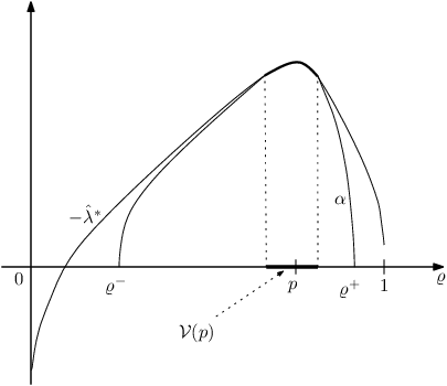
The function (−λ^∗)(-{\hat{\lambda}}^{*}) is important for understanding the rate α{\alpha}. (We recall that both functions depend on pp, but we don’t write explicitely the dependence.) Note that these two functions coincide at ϱ=p\varrho=p and take the value ln⁡(2​d)\ln(2d).

Theorem 1.3

Let p∈(0,1)p\in(0,1).

  1. 1.

    We have the annealed bound: For all ϱ\varrho,

    α⁡(ϱ)≤−λ^∗​(ϱ).{\alpha}(\varrho)\leq-{\hat{\lambda}}^{*}(\varrho)\;. (8)
  2. 2.

    The function α⁡(ϱ)+λ^∗​(ϱ){\alpha}(\varrho)+{\hat{\lambda}}^{*}(\varrho) is nonincreasing for ϱ∈[p,ϱ+)\varrho\in[p,\varrho^{+}) and is nondecreasing for ϱ∈(ϱ−,p]\varrho\in(\varrho^{-},p].

  3. 3.

    The set

    𝒱⁡(p)={ϱ∈(0,1):α⁡(ϱ)=−λ^∗​(ϱ)}{\mathcal{V}}(p)=\{\varrho\in(0,1):{\alpha}(\varrho)=-{\hat{\lambda}}^{*}(\varrho)\} (9)

    is an interval containing pp (here, “interval” is understood in broad sense, i.e., it can reduce to the single point {p}\{p\}).

  4. 4.

    In dimension d=1d=1, 𝒱⁡(p)={p}{\mathcal{V}}(p)=\{p\}, i.e. the inequality in (8) is strict for all ϱ≠p\varrho\neq p.

  5. 5.

    In dimension d≥3d\geq 3, 𝒱⁡(p){\mathcal{V}}(p) contains a neighborhood of pp.

  6. 6.

    Let d≥3d\geq 3, and πd\pi_{d} be the probability for the dd-dimensional simple random walk to ever return to the starting point. When p>πdp>\pi_{d}, then [p,1)⊂𝒱⁡(p)[p,1)\subset{\mathcal{V}}(p), so that the equality holds in (8) for all ϱ∈[p,1)\varrho\in[p,1). Similarly, when p<1−πdp<1-\pi_{d}, then (0,p]⊂𝒱⁡(p)(0,p]\subset{\mathcal{V}}(p), so that the equality holds for all ϱ∈(0,p]\varrho\in(0,p].

  7. 7.

    In dimension d≥2d\geq 2, if p<(1/2​d)p<(1/2d), then sup𝒱⁡(p)<1\sup{\mathcal{V}}(p)<1. Similarly, if p>1−(1/2​d)p>1-(1/2d), we have inf𝒱⁡(p)>0\inf{\mathcal{V}}(p)>0.

Remark 1.4

(i) The annealed bound comes from the first-moment method, and most of the results stating that the equality α⁡(ϱ)=−λ^∗​(ϱ){\alpha}(\varrho)=-{\hat{\lambda}}^{*}(\varrho) holds, are derived from the second-moment method.

(ii) By transience of the random walk in dimension d≥3d\geq 3, we have πd<1\pi_{d}<1. In fact, π3=0.3404​…>π4>π5​…\pi_{3}=0.3404\ldots>\pi_{4}>\pi_{5}\ldots [23, page 103]. In particular, for p∈(πd,1−πd)p\in(\pi_{d},1-\pi_{d}), we have α⁡(ϱ)=−λ^∗​(ϱ){\alpha}(\varrho)=-{\hat{\lambda}}^{*}(\varrho) for all ϱ∈(0,1)\varrho\in(0,1).

Refer to caption
Figure 2: Typical behaviour of the function α\alpha when d≥3d\geq 3

The following property of the free energy φ\varphi of the directed polymer is interesting and seems to be new.

Theorem 1.5

The function φ\varphi is strictly convex on ℝ{\mathbb{R}}, and the functions φ∗\varphi^{*} and α{\alpha} are differentiable in the interior of their domains.

We will obtain much sharper results for large dimension and ϱ\varrho’s not too far from pp. The reason is that the partition function ZnZ_{n} behaves smoothly as n↗∞n\nearrow{\infty}. The almost-sure limit

W∞​(β)=limn→∞Zn​(β)​e−n​λ^​(β)W_{\infty}({\beta})=\lim_{n\to{\infty}}Z_{n}({\beta})e^{-n{\hat{\lambda}}({\beta})}

exists for all β{\beta}, since the sequence is a positive (𝒢n)n({\mathcal{G}}_{n})_{n}-martingale, where 𝒢n=σ⁡{η⁡(t,x);t≤n,x∈ℤd}{\mathcal{G}}_{n}=\sigma\{{\eta}(t,x);t\leq n,x\in{\mathbb{Z}}^{d}\}. So, let us now concentrate on the case of large dimension, d≥3d\geq 3. When β{\beta} belongs to some neighborhood of the origin (known as the weak disorder region), the limit W∞W_{\infty} is strictly positive a.s. In a smaller neighborhood of the origin, the limit can be expressed as a (random) perturbation series in ℒ2{\mathcal{L}}^{2} [22]. Moreover, the convergence holds in much stronger sense, namely, in the sense of analytic functions [7]. We will use strong tools from complex analysis, as it is classically done to obtain limit theorems for sums of random variables [20].

Theorem 1.6

Assume d≥3d\geq 3. There exist a neighborhood U3U_{3} of pp in ℝ{\mathbb{R}} and an event Ω2\Omega_{2} with full probability such that for every sequence knk_{n} with kn/n→ϱ∈U3k_{n}/n\to\varrho\in U_{3} and all η∈Ω2{\eta}\in\Omega_{2},

Qn​(kn)=−α′′​(ϱ)2​π​n​W∞​(β⁡(ϱ))​exp⁡{n​α​(knn)}​(1+o⁡(1))Q_{n}(k_{n})=\sqrt{\frac{-{\alpha}^{\prime\prime}(\varrho)}{2\pi n}}\;W_{\infty}({\beta}(\varrho))\;\exp\Big\{n{\alpha}\Big(\frac{k_{n}}{n}\Big)\Big\}\;(1+o(1))

where o⁡(1)o(1) tends to 0 as n→∞n\to{\infty}, and β⁡(ϱ)=ln⁡(1−p)​ϱp⁡(1−ϱ){\beta}(\varrho)=\ln\frac{(1-p)\varrho}{p(1-\varrho)}. The neighborhood U3U_{3} is contained in 𝒱⁡(p){\mathcal{V}}(p), hence we have α=−λ^∗{\alpha}=-{\hat{\lambda}}^{*} with λ^∗{\hat{\lambda}}^{*} given by (7).

We note that the leading order is deterministic, but the prefactor is random (as W∞W_{\infty}), depending on the particular realization of the Bernoulli field. This theorem is a corollary of a more refined result (Theorem 3.2), which can be found in Section 3. This will be proved by complex analysis arguments, considering the Fourier transform of HnH_{n} under some (polymer) measure. Fourier methods are quite strong, they are used in a different spirit in [1] to obtain sharp results on the polymer path itself for small β{\beta}. The disadvantage is that we have to restrict the parameter domain. It would be tempting to use only real variable techniques as in the Ornstein-Zernike theory for the Bernoulli bond percolation [3], but we take another, shorter route.

Remark 1.7

The model is also interesting with real-valued η⁡(t,x){\eta}(t,x) with general distribution. This is motivated by first-passage time percolation. Our results at the exponential order remain valid for variables with exponential moments. For the case of the Gaussian law, we mention the recent preprint [17] on the so-called REM conjecture: it is proved that the local statistics of (Hn​(S),S∈𝒫n)(H_{n}(S);S\in{\mathcal{P}}_{n}) approach that of a Poisson point process, provided that one focuses on values distant from the mean 𝔼​Hn{\mathbb{E}}H_{n} by at most o⁡(n1−ε)o(n^{1-\varepsilon}).

We can interpret our last result in this spirit. In our case, (Hn​(S),S∈𝒫n)(H_{n}(S);S\in{\mathcal{P}}_{n}) spreads on the lattice, and natural local statistics of the energy levels are the ratios Qn​(kn)/𝔼​Qn​(kn)Q_{n}(k_{n})/{\mathbb{E}}Q_{n}(k_{n}). For d≥3d\geq 3 and kn∼n​ϱ∈U3k_{n}\sim n\varrho\in U_{3},

Qn​(kn)/𝔼​Qn​(kn)≃W∞​(β⁡(ϱ))Q_{n}(k_{n})/{\mathbb{E}}Q_{n}(k_{n})\simeq W_{\infty}({\beta}(\varrho))

since 𝔼​W∞​(β)=1{\mathbb{E}}W_{\infty}({\beta})=1. We emphasize that here the energy level knk_{n} is of order nn (far from the bulk), and that the limit is not universal but depends on the lattice and the law of the environment η{\eta}.

2 Logarithmic asymptotics

2.1 Proof of Theorem 1.1

We start by introducing some probability measures.

Let PP be the law of the simple random walk on ℤd{\mathbb{Z}}^{d} starting from 0, i.e. the probability measure on the space 𝒫∞{\mathcal{P}}_{\infty} of infinite paths making the increments St−St−1S_{t}-S_{t-1} independent and uniformly distributed on the set of 2​d2d neighbors of 0∈ℤd0\in{\mathbb{Z}}^{d}. Observe that the restriction of PP to paths of length nn is the normalized counting measure on 𝒫n{\mathcal{P}}_{n}, and so the partition function takes now the familiar form (EPE_{P} is the expectation with respect to PP)

Zn=(2​d)n​EP​[exp⁡{β​Hn​(S)}].Z_{n}=(2d)^{n}E_{P}[\exp\{{\beta}H_{n}(S)\}]. (10)

The law νn=νnη\nu_{n}=\nu_{n}^{{\eta}} of (1/n)​Hn(1/n)H_{n} under PP, given by νn​({ϱ}):=P⁡(Hn​(S)=n​ϱ)\nu_{n}(\{\varrho\}):=P(H_{n}(S)=n\varrho), is such that

νn​({ϱ})=Qn​(n​ϱ)(2​d)nifn​ϱ∈{0,1,…,n}.\nu_{n}(\{\varrho\})=\frac{Q_{n}(n\varrho)}{(2d)^{n}}\hskip 10.00002pt{\rm if}\hskip 10.00002ptn\varrho\in\{0,1,\ldots,n\}. (11)

We extend νn\nu_{n} to a probability measure on ℝ{\mathbb{R}} that we still denote by νn\nu_{n}, νn​(A)=∑ϱ∈A,n​ϱ∈{0,1,…,n}νn​({ϱ}),A⊂ℝ\nu_{n}(A)=\sum_{\varrho\in A,n\varrho\in\{0,1,\ldots,n\}}\nu_{n}(\{\varrho\}),A\subset{\mathbb{R}}.

All what we need to obtain the proof of Theorem 1.1, is to prove that νn\nu_{n} obeys an almost sure large deviation principle, see Proposition 2.1 below. Recall first the event Ω0​(β)\Omega_{0}({\beta}) from (4), and define the event Ω0=⋂β∈ℚΩ0​(β)\Omega_{0}=\bigcap_{{\beta}\in{\mathbb{Q}}}\Omega_{0}({\beta}). Then, we have ℙ⁡(Ω0)=1{\mathbb{P}}(\Omega_{0})=1, and on this event the convergence (4) holds for any real number β{\beta} by convexity and monotonicity.

Proposition 2.1

The function

I⁡(ϱ)=ln⁡(2​d)+φ∗​(ϱ)∈[0,ln⁡(2​d)]∪{+∞}I(\varrho)=\ln(2d)+\varphi^{*}(\varrho)\in[0,\ln(2d)]\cup\{+{\infty}\}

is lower semi-continuous and convex on [0,1][0,1]. Moreover, for all η∈Ω0{\eta}\in\Omega_{0} the sequence (νn,n≥1)(\nu_{n},n\geq 1) obeys a large deviation principle with rate function II. That is,

  • (i)

    for any closed F⊂[0,1]F\subset[0,1], we have

    lim supn→∞n−1lnνn(F)≤−infϱ∈FI(ϱ),\limsup_{n\to{\infty}}n^{-1}\ln\nu_{n}(F)\leq-\inf_{\varrho\in F}I(\varrho),
  • (ii)

    for any open (in the induced topology on [0,1][0,1]) G⊂[0,1]G\subset[0,1], we have

    lim infn→∞n−1lnνn(G)≥−infϱ∈GI(ϱ).\liminf_{n\to{\infty}}n^{-1}\ln\nu_{n}(G)\geq-\inf_{\varrho\in G}I(\varrho).

Now, we first finish the proof of Theorem 1.1, and then prove the above proposition.

Proof of Theorem 1.1. Assume that ϱ∈[p,ϱ+)\varrho\in[p,\varrho^{+}) and η∈Ω0{\eta}\in\Omega_{0}. Applying (i) of Proposition 2.1 with F=[ϱ,1]F=[\varrho,1] and using (11) together with the fact that ϱ≥p\varrho\geq p, we see that the limit in (6) is not larger than ln⁡(2​d)−I⁡(ϱ)=α⁡(ϱ)\ln(2d)-I(\varrho)={\alpha}(\varrho). Applying (ii) of Proposition 2.1 with G=(ϱ+ε,1]G=(\varrho+\varepsilon,1] (ε>0\varepsilon>0) and using the fact that ϱ≥p\varrho\geq p, we see that the limit is at least α⁡(ϱ+ε){\alpha}(\varrho+\varepsilon). Since ϱ<ϱ+\varrho<\varrho^{+}, this quantity tends to α⁡(ϱ){\alpha}(\varrho) as ε↘0\varepsilon\searrow 0. This proves (6) for ϱ∈[p,ϱ+)\varrho\in[p,\varrho^{+}). The case ϱ∈(ϱ−,p)\varrho\in(\varrho^{-},p) is completely similar. Finally, when ϱ>ϱ+\varrho>\varrho^{+} (the case ϱ<ϱ−\varrho<\varrho^{-} is similar) we have I⁡(ϱ)=∞I(\varrho)={\infty} and then Rn​(ϱ)=0R_{n}(\varrho)=0 for large nn, proving (6) in this case. □\Box

Proof of Proposition 2.1. The properties of II are clear from the definition.

Fix η∈Ω0{\eta}\in\Omega_{0}. In view of (4) and (10), the Laplace transforms of νn(⋅)=P((1/n)Hn=⋅)\nu_{n}(\cdot)=P((1/n)H_{n}=\cdot) have logarithmic asymptotics:

limn→∞1n​ln⁡EP​(exp⁡{β​Hn​(S)})=φ⁡(β)−ln⁡(2​d)\lim_{n\to{\infty}}\frac{1}{n}\ln E_{P}(\exp\{{\beta}H_{n}(S)\})=\varphi({\beta})-\ln(2d)

for all real β{\beta}. From the Gärtner-Ellis theorem (Theorem 2.3.6 in [9]), the full statement (i) in Proposition 2.1 follows, and we obtain for open G⊂[0,1]G\subset[0,1] that

lim infn→∞1nlnνn(G)≥−inf{I(ϱ);ϱ∈G∩ℰ},\liminf_{n\to{\infty}}\frac{1}{n}\ln\nu_{n}(G)\geq-\inf\{I(\varrho);\varrho\in G\cap{\mathcal{E}}\}\;, (12)

where

ℰ={ϱ∈[0,1]:∃β∀r≠ϱ,βϱ−φ∗(ϱ)>βr−φ∗(r)}{\mathcal{E}}=\Big\{\varrho\in[0,1]:\exists\beta\;\forall r\neq\varrho,\;\beta\varrho-\varphi^{*}(\varrho)>\beta r-\varphi^{*}(r)\Big\}

is the set of exposed points of φ∗\varphi^{*} from (5). Its complement is the set of all points ϱ\varrho such that φ∗\varphi^{*} is linear in a neighborhood of ϱ\varrho. We will improve (12) into (ii) of Proposition 2.1 with a subadditivity argument. We start by showing that φ\varphi is differentiable at 0 with that φ′​(0)=p\varphi^{\prime}(0)=p. Indeed, using Jensen inequality twice, we have

1n​ln​EP​[e𝔼​β​(Hn−n​p)]≤𝔼​1n​ln​EP​[eβ⁡(Hn−n​p)]≤1n​ln​𝔼​EP​[eβ⁡(Hn−n​p)]\frac{1}{n}\ln E_{P}[e^{{\mathbb{E}}{\beta}(H_{n}-np)}]\leq{\mathbb{E}}\frac{1}{n}\ln E_{P}[e^{{\beta}(H_{n}-np)}]\leq\frac{1}{n}\ln{\mathbb{E}}E_{P}[e^{{\beta}(H_{n}-np)}]

Computing the extreme terms and taking the limit n→∞n\to{\infty} for the middle one, we get

0≤φ⁡(β)−β​p≤λ⁡(β)−β​p,0\leq\varphi({\beta})-{\beta}p\leq{\lambda}({\beta})-{\beta}p\;,

which shows that φ′​(0)=p\varphi^{\prime}(0)=p since λ′​(0)=p{\lambda}^{\prime}(0)=p. This implies that p∈ℰp\in{\mathcal{E}} and that ℰ{\mathcal{E}} is a neighborhood of pp. Let ϱ∈(ϱ−,ϱ+)∩G\varrho\in(\varrho^{-},\varrho^{+})\cap G be a non-exposed point of φ∗\varphi^{*}. For definiteness, we assume ϱ>p\varrho>p. Let

ϱ1=sup{ϱ′∈ℰ;ϱ′<ϱ},ϱ2=inf{ϱ′∈ℰ;ϱ′>ϱ}.\varrho_{1}=\sup\{\varrho^{\prime}\in{\mathcal{E}};\varrho^{\prime}<\varrho\}\;,\hskip 10.00002pt\varrho_{2}=\inf\{\varrho^{\prime}\in{\mathcal{E}};\varrho^{\prime}>\varrho\}\;.

Recall that φ\varphi is strictly convex by Theorem 1.5 – that we will prove below independently. This implies that the function φ∗\varphi^{*} cannot have a linear piece that goes up to ϱ+\varrho^{+}, cf. Figure 1. Then, p<ϱ1<ϱ<ϱ2<ϱ+p<\varrho_{1}<\varrho<\varrho_{2}<\varrho^{+}, and ϱ1,ϱ2∈ℰ\varrho_{1},\varrho_{2}\in{\mathcal{E}}. Let γ∈(0,1)\gamma\in(0,1) such that ϱ=γ​ϱ1+(1−γ)​ϱ2\varrho=\gamma\varrho_{1}+(1-\gamma)\varrho_{2}. Since the interval (ϱ1,ϱ2)(\varrho_{1},\varrho_{2}) consists of non-exposed points, we have I⁡(ϱ)=γ​I​(ϱ1)+(1−γ)​I​(ϱ2)I(\varrho)=\gamma I(\varrho_{1})+(1-\gamma)I(\varrho_{2}). Since GG is open and contains ϱ\varrho, we can find ε>0\varepsilon>0 and k,ℓ∈ℕ∗k,\ell\in{\mathbb{N}}^{*} such that

|u−ϱ1|<ε,|v−ϱ2|<ε⟹k​u+ℓ​vk+ℓ∈Gε|u-\varrho_{1}|<\varepsilon,|v-\varrho_{2}|<\varepsilon\Longrightarrow\frac{ku+\ell v}{k+\ell}\in G^{\varepsilon}

with GεG^{\varepsilon} the set of r∈Gr\in G at distance at least ε\varepsilon from the outside of GG. The key fact is

Card{S∈𝒫n⁡(k+ℓ):Hn⁡(k+ℓ)​(S)n⁡(k+ℓ)∈Gε}\displaystyle\mathop{\rm Card}\nolimits\Big\{S\in{\mathcal{P}}_{n(k+\ell)}:\frac{H_{n(k+\ell)}(S)}{n(k+\ell)}\in G^{\varepsilon}\Big\}
≥\displaystyle\geq ∑x∈ℤdCard{S∈𝒫n⁡(k+ℓ):Hn​k​(S)n​k∈(ϱ1−ε,ϱ1+ε),Sn​k=x}\displaystyle\sum_{x\in{\mathbb{Z}}^{d}}\mathop{\rm Card}\nolimits\Big\{S\in{\mathcal{P}}_{n(k+\ell)}:\frac{H_{nk}(S)}{nk}\in(\varrho_{1}-\varepsilon,\varrho_{1}+\varepsilon),S_{nk}=x\Big\}
×Card{S∈𝒫n⁡(k+ℓ):Sn​k=x,\displaystyle{}\times\mathop{\rm Card}\nolimits\Big\{S\in{\mathcal{P}}_{n(k+\ell)}:S_{nk}=x,
Hn⁡(k+ℓ)​(S)−Hn​k​(S)n​ℓ∈(ϱ2−ε,ϱ2+ε)}\displaystyle~~~~~~~~~~~~~~~\frac{H_{n(k+\ell)}(S)-H_{nk}(S)}{n\ell}\in(\varrho_{2}-\varepsilon,\varrho_{2}+\varepsilon)\Big\}
≥\displaystyle\geq Card{S∈𝒫n⁡(k+ℓ):Hn​k​(S)n​k∈(ϱ1−ε,ϱ1+ε)}\displaystyle\mathop{\rm Card}\nolimits\Big\{S\in{\mathcal{P}}_{n(k+\ell)}:\frac{H_{nk}(S)}{nk}\in(\varrho_{1}-\varepsilon,\varrho_{1}+\varepsilon)\Big\}
×min‖x‖1≤n​kCard{S∈𝒫n⁡(k+ℓ):Sn​k=x,\displaystyle{}\times\min_{\|x\|_{1}\leq nk}\mathop{\rm Card}\nolimits\Big\{S\in{\mathcal{P}}_{n(k+\ell)}:S_{nk}=x,
Hn⁡(k+ℓ)​(S)−Hn​k​(S)n​ℓ∈(ϱ2−ε,ϱ2+ε)}\displaystyle~~~~~~~~~~~~~~~~~~~~~~~~~~\frac{H_{n(k+\ell)}(S)-H_{nk}(S)}{n\ell}\in(\varrho_{2}-\varepsilon,\varrho_{2}+\varepsilon)\Big\}
=\displaystyle= Card{S∈𝒫n​k:Hn​k​(S)n​k∈(ϱ1−ε,ϱ1+ε)}\displaystyle\mathop{\rm Card}\nolimits\Big\{S\in{\mathcal{P}}_{nk}:\frac{H_{nk}(S)}{nk}\in(\varrho_{1}-\varepsilon,\varrho_{1}+\varepsilon)\Big\}
×min⁡Card‖x‖1≤n​k⁡{S∈𝒫n​ℓ:Hn​ℓ(n​k,x)​(S)n​ℓ∈(ϱ2−ε,ϱ2+ε)}\displaystyle{}\times\min_{\|x\|_{1}\leq nk}\mathop{\rm Card}\nolimits\Big\{S\in{\mathcal{P}}_{n\ell}:\frac{H_{n\ell}^{(nk,x)}(S)}{n\ell}\in(\varrho_{2}-\varepsilon,\varrho_{2}+\varepsilon)\Big\}

with Hn​ℓ(n​k,x)​(S)=∑t=1nη⁡(t+n​k,St+x)H_{n\ell}^{(nk,x)}(S)=\sum_{t=1}^{n}{\eta}(t+nk,S_{t}+x) the Hamiltonian in the time-space shifted environment. Similarly, we denote by νn​ℓ(n​k,x)\nu_{n\ell}^{(nk,x)} the measure νn​ℓ(n​k,x)(⋅)=P(Hn​ℓ(n​k,x)∈⋅)\nu_{n\ell}^{(nk,x)}(\cdot)=P(H_{n\ell}^{(nk,x)}\in\cdot). The above display implies that

lim infn→∞1n⁡(k+ℓ)​ln⁡νn⁡(k+ℓ)​(Gε)\displaystyle\liminf_{n\to{\infty}}\frac{1}{n(k+\ell)}\ln\nu_{n(k+\ell)}(G^{\varepsilon})
≥\displaystyle\geq kk+ℓ​lim infn→∞1n​k​ln⁡νn​k​((,,,))\displaystyle\frac{k}{k+\ell}\liminf_{n\to{\infty}}\frac{1}{nk}\ln\nu_{nk}\big((\varrho_{1}-\varepsilon,\varrho_{1}+\varepsilon)\big)
+ℓk+ℓlim infn→∞1n​ℓmin‖x‖1≤n​klnνn​ℓ(n​k,x)((ϱ2−ε,ϱ2+ε))\displaystyle{}+\frac{\ell}{k+\ell}\liminf_{n\to{\infty}}\frac{1}{n\ell}\min_{\|x\|_{1}\leq nk}\ln\nu_{n\ell}^{(nk,x)}\big((\varrho_{2}-\varepsilon,\varrho_{2}+\varepsilon)\big)

It is straightforward to check that

lim infn→∞1n⁡(k+ℓ)​ln⁡νn⁡(k+ℓ)​(Gε)≤lim infn→∞1n​ln⁡νn​(G),\liminf_{n\to{\infty}}\frac{1}{n(k+\ell)}\ln\nu_{n(k+\ell)}(G^{\varepsilon})\leq\liminf_{n\to{\infty}}\frac{1}{n}\ln\nu_{n}(G)\;,

and it is not difficult to see that

lim infn→∞1n​ℓ​min‖x‖1≤n​k​ln⁡νn​ℓ(n​k,x)​((,,,))≥−I⁡(ϱ2),ℙ-a.s.\liminf_{n\to{\infty}}\frac{1}{n\ell}\min_{\|x\|_{1}\leq nk}\ln\nu_{n\ell}^{(nk,x)}\big((\varrho_{2}-\varepsilon,\varrho_{2}+\varepsilon)\big)\geq-I(\varrho_{2})\;,\hskip 10.00002pt\text{${\mathbb{P}}$-a.s.} (13)

We postpone the proof of (13) for the moment. Hence, the key inequality implies

lim infn→∞1n​ln⁡νn​(G)\displaystyle\liminf_{n\to{\infty}}\frac{1}{n}\ln\nu_{n}(G) ≥\displaystyle\geq −kk+ℓ​I​(ϱ1+ε)−ℓk+ℓ​I​(ϱ2+ε),\displaystyle-\frac{k}{k+\ell}I(\varrho_{1}+\varepsilon)-\frac{\ell}{k+\ell}I(\varrho_{2}+\varepsilon)\;,
lim infn→∞1n​ln⁡νn​(G)\displaystyle\liminf_{n\to{\infty}}\frac{1}{n}\ln\nu_{n}(G) ≥\displaystyle\geq −[γ​I​(ϱ1)+(1−γ)​I​(ϱ2)]=−I⁡(ϱ),\displaystyle-\big[\gamma I(\varrho_{1})+(1-\gamma)I(\varrho_{2})\big]=-I(\varrho),

letting ε↘0\varepsilon\searrow 0 and k/(k+ℓ)→γk/(k+\ell)\to\gamma. This yields statement (ii) in Proposition 2.1.

Now, let us prove (13). By a standard concentration inequality (e.g., Theorem 4.2 in [6]), we have

ℙ⁡(|ln⁡Zn−𝔼​ln⁡Zn|≥u)≤2​exp⁡{−u24​β2​n}.{\mathbb{P}}(|\ln Z_{n}-{\mathbb{E}}\ln Z_{n}|\geq u)\leq 2\exp\Big\{-\frac{u^{2}}{4{\beta}^{2}n}\Big\}\;.

Therefore we have, ℙ{\mathbb{P}}-a.s. as n→∞n\to{\infty},

max‖x‖1≤m≤n⁡|1n​ln⁡Zn(m,x)​(β)−φ⁡(β)|→0,β∈ℝ,\max_{\|x\|_{1}\leq m\leq n}\Big|\frac{1}{n}\ln Z_{n}^{(m,x)}({\beta})-\varphi({\beta})\Big|\to 0\;,\hskip 10.00002pt{\beta}\in{\mathbb{R}}\;,

with Zn(m,x)Z_{n}^{(m,x)} the partition function associated to Hn(m,x)H_{n}^{(m,x)}. Since ϱ2\varrho_{2} is an exposed point for φ∗\varphi^{*}, (13) follows from the Gärtner-Ellis theorem. □\Box

Let us comment on the above proof. We could improve (12) into the full lower bound (ii) in Proposition 2.1 with a subadditivity argument, implying convexity of the rate function. If we knew that (ϱ−,ϱ+)⊂ℰ(\varrho^{-},\varrho^{+})\subset{\mathcal{E}} – or, equivalently, that φ\varphi is differentiable –, we could directly conclude without this extra argument. We tried to prove it, but we could not. We state it as a conjecture:

Conjecture 2.2

The function φ\varphi is everywhere differentiable.

2.2 Proof of Theorem 1.3

  1. 1.

    By Jensen inequality,

    𝔼​ln⁡Zn≤n​λ^​(β).{\mathbb{E}}\ln Z_{n}\leq n{\hat{\lambda}}({\beta})\;.

    Then, φ​(β)≤λ^​(β)\varphi({\beta})\leq{\hat{\lambda}}({\beta}), which implies φ∗​(ϱ)≥λ^∗​(ϱ)\varphi^{*}(\varrho)\geq{\hat{\lambda}}^{*}(\varrho) from the definition of Legendre transform. The inequality now follows from α≤−φ∗{\alpha}\leq-\varphi^{*}.

  2. 2.

    Set φn​(β)=n−1​𝔼​ln⁡Zn​(β)\varphi_{n}(\beta)=n^{-1}{\mathbb{E}}\ln Z_{n}(\beta). From Theorem 1.1 in [7] we have

    λ^′​(β)≥φn′​(β){\hat{\lambda}}^{\prime}(\beta)\geq\varphi_{n}^{\prime}(\beta)

    for all β≥0\beta\geq 0. Hence, for ϱ≥p\varrho\geq p, the reciprocal functions are such that

    (λ^′)−1​(ϱ)≤(φn′)−1​(ϱ).({\hat{\lambda}}^{\prime})^{-1}(\varrho)\leq(\varphi_{n}^{\prime})^{-1}(\varrho)\;.

    Since (λ^′)−1=(λ^∗)′({\hat{\lambda}}^{\prime})^{-1}=({\hat{\lambda}}^{*})^{\prime} and (φn′)−1=(φn∗)′(\varphi_{n}^{\prime})^{-1}=(\varphi_{n}^{*})^{\prime}, we have

    (λ^∗)′​(ϱ)≤(φ∗)′​(ϱ)({\hat{\lambda}}^{*})^{\prime}(\varrho)\leq(\varphi^{*})^{\prime}(\varrho)

    for all ϱ≥p\varrho\geq p where φ∗\varphi^{*} is differentiable. Since α=−φ∗\alpha=-\varphi^{*} for ϱ≠ϱ+\varrho\neq\varrho^{+}, this proves the first half of the desired statement. The other half is similar.

  3. 3.

    From Theorem 1.1 in [7] it is known that the set

    𝒲⁡(p)={β∈ℝ:φ⁡(β)=λ^​(β)}{\mathcal{W}}(p)=\{\beta\in{\mathbb{R}}:\varphi({\beta})={\hat{\lambda}}({\beta})\}

    is an interval containing 0. Let β∈𝒲⁡(p){\beta}\in{\mathcal{W}}(p), and ϱ=λ′​(β)=λ^′​(β)\varrho={\lambda}^{\prime}({\beta})={\hat{\lambda}}^{\prime}({\beta}). From Theorem 2.3 (a) in [4] it is known that β∈𝒲⁡(p)\beta\in{\mathcal{W}}(p) implies φ∗​(ϱ)≤0\varphi^{*}(\varrho)\leq 0. Then, the supremum defining λ^∗​(ϱ){\hat{\lambda}}^{*}(\varrho) is achieved at β{\beta}, which implies the first equality in

    −λ^∗​(ϱ)=−[β​ϱ−λ^​(β)]=−[β​ϱ−φ⁡(β)]=−φ∗​(ϱ)=α⁡(ϱ),\displaystyle-{\hat{\lambda}}^{*}(\varrho)=-[{\beta}\varrho-{\hat{\lambda}}({\beta})]=-[{\beta}\varrho-\varphi({\beta})]=-\varphi^{*}(\varrho)={\alpha}(\varrho)\;,

    where the second equality holds for β∈𝒲⁡(p){\beta}\in{\mathcal{W}}(p), the third one because of φ′​(β)=λ^′​(β)=ϱ\varphi^{\prime}({\beta})={\hat{\lambda}}^{\prime}({\beta})=\varrho, and the last one because φ∗​(ϱ)≤0\varphi^{*}(\varrho)\leq 0.

    Let now β∉𝒲⁡(p){\beta}\notin{\mathcal{W}}(p), and ϱ=λ′​(β)\varrho={\lambda}^{\prime}({\beta}). Then,

    −λ^∗​(ϱ)=−[β​ϱ−λ^​(β)]>−[β​ϱ−φ⁡(β)]≥−φ∗​(ϱ)≥α⁡(ϱ).\displaystyle-{\hat{\lambda}}^{*}(\varrho)=-[{\beta}\varrho-{\hat{\lambda}}({\beta})]>-[{\beta}\varrho-\varphi({\beta})]\geq-\varphi^{*}(\varrho)\geq{\alpha}(\varrho)\;.

    Observe that λ′{\lambda}^{\prime} is a diffeomorphism from ℝ{\mathbb{R}} to (0,1)(0,1). From this we can identify the set 𝒱⁡(p){\mathcal{V}}(p) defined by (9),

    𝒱⁡(p)={λ′​(β);β∈𝒲⁡(p)},{\mathcal{V}}(p)=\{{\lambda}^{\prime}({\beta});{\beta}\in{\mathcal{W}}(p)\}\;, (14)

    which is an interval containing pp.

  4. 4.

    When d=1d=1, it is known that 𝒲⁡(p)={0}{\mathcal{W}}(p)=\{0\}, see Theorem 1.1 in [7]. Hence, 𝒱⁡(p){\mathcal{V}}(p) reduces to {p}\{p\}.

  5. 5.

    When d≥3d\geq 3, from celebrated results of Imbrie and Spencer [13], Bolthausen [2], it is known that 𝒲⁡(p){\mathcal{W}}(p) contains a neighborhood of 0. In view of (14), 𝒱⁡(p){\mathcal{V}}(p) is in its turn a neighborhood of pp.

  6. 6.

    This is a consequence of [5, example 2.1.1], which shows for instance that, if p>πdp>\pi_{d}, then 𝒲⁡(p)⊃ℝ+{\mathcal{W}}(p)\supset{\mathbb{R}}^{+}. Indeed, in view of (14), this implies that 𝒱⁡(p){\mathcal{V}}(p) contains [p,1)[p,1), and α{\alpha} is still equal to −λ^∗-{\hat{\lambda}}^{*} at ϱ=1\varrho=1 by upper semi-continuity of both functions. The case of p<1−πdp<1-\pi_{d} is similar.

  7. 7.

    This is a consequence of [5, example 2.2.1], which shows for instance that, if p<(1/2​d)p<(1/2d), then 𝒲⁡(p){\mathcal{W}}(p) is bounded from above. The other case is similar.

□\Box

2.3 Strict convexity of the free energy

The aim of this section is to prove Theorem 1.5. We start with a variance estimate analogous to that for Gibbs field in [10].

Lemma 2.3

For any compact set K⊂ℝK\subset{\mathbb{R}}, there exists a positive constant C=CKC=C_{K} such that

𝔼​(ln⁡Zn)′′​(β)≥C​n,β∈K{\mathbb{E}}(\ln Z_{n})^{\prime\prime}({\beta})\geq Cn\;,\hskip 20.00003pt{\beta}\in K

Proof: The polymer measure at inverse temperature β{\beta} with environment η{\eta} is the random probability measure μn=μnβ\mu_{n}=\mu_{n}^{\beta} on the path space defined by

μn​({S})=Zn−1​exp⁡{β​Hn​(S)},S=(S1,…,Sn)∈𝒫n.\mu_{n}(\{S\})=Z_{n}^{-1}\exp\{{\beta}H_{n}(S)\}\;,\hskip 10.00002ptS=(S_{1},\ldots,S_{n})\in{\mathcal{P}}_{n}\;. (15)

For simplicity we write μn​(S1,…,Sn)\mu_{n}(S_{1},\ldots,S_{n}) for μn​({(S1,…,Sn)})\mu_{n}(\{(S_{1},\ldots,S_{n})\}). The polymer measure is Markovian (but time-inhomogeneous), and

(ln⁡Zn)′′​(β)=Varμn​(Hn).(\ln Z_{n})^{\prime\prime}({\beta})={\rm Var}_{\mu_{n}}(H_{n}).

Let Σt{\Sigma}_{t} be the tt-coordinate mapping on 𝒫n{\mathcal{P}}_{n} given by Σt​(S)=St{\Sigma}_{t}(S)=S_{t}, and regard it as a random variable.

Define

ℐ⁡(x,y)={z∈ℤd:‖x−z‖1=‖z−y‖1=1},x,y∈ℤd{\mathcal{I}}(x,y)=\{z\in{\mathbb{Z}}^{d}:\|x-z\|_{1}=\|z-y\|_{1}=1\}\;,\hskip 10.00002ptx,y\in{\mathbb{Z}}^{d} (16)

the set of lattice points which are next to both xx and yy. The set ℐ⁡(x,y){\mathcal{I}}(x,y) is empty except if yy can be reached in two steps by the simple random walk from xx; in this case its cardinality is equal to 2​d,22d,2 or 1 according to y=x,‖y−x‖∞=1y=x,\|y-x\|_{\infty}=1 or ‖y−x‖∞=2\|y-x\|_{\infty}=2. The Markov property implies that, under μ2​n\mu_{2n}, Σ1,Σ3,…,Σ2​n−1{\Sigma}_{1},{\Sigma}_{3},\ldots,{\Sigma}_{2n-1} are independent conditionally on Σe:=(Σ2,Σ4,…,Σ2​n){\Sigma}^{e}:=({\Sigma}_{2},{\Sigma}_{4},\ldots,{\Sigma}_{2n}), and the law of Σ2​t−1{\Sigma}_{2t-1} given Σe{\Sigma}^{e} only depends on Σ2​t−2,Σ2​t{\Sigma}_{2t-2},{\Sigma}_{2t}, and has support ℐ⁡(Σ2​t−2,Σ2​t){\mathcal{I}}({\Sigma}_{2t-2},{\Sigma}_{2t}).

From the variance decomposition under conditioning, we have

Varμ2​n​(H2​n)\displaystyle{\rm Var}_{\mu_{2n}}(H_{2n}) =\displaystyle= Eμ2​n​Varμ2​n​(H2​n∣Σe)+Varμ2​n​(Eμ2​n​[H2​n∣Σe])\displaystyle E_{\mu_{2n}}{\rm Var}_{\mu_{2n}}(H_{2n}\mid{\Sigma}^{e})+{\rm Var}_{\mu_{2n}}(E_{\mu_{2n}}[H_{2n}\mid{\Sigma}^{e}])
≥\displaystyle\geq Eμ2​n​Varμ2​n​(H2​n∣Σe)\displaystyle E_{\mu_{2n}}{\rm Var}_{\mu_{2n}}(H_{2n}\mid{\Sigma}^{e})
=\displaystyle= Eμ2​n​Varμ2​n​(∑t=1nη⁡(2​t−1,Σ2​t−1)∣Σe)\displaystyle E_{\mu_{2n}}{\rm Var}_{\mu_{2n}}(\sum_{t=1}^{n}{\eta}(2t-1,{\Sigma}_{2t-1})\mid{\Sigma}^{e})
=\displaystyle= ∑t=1nEμ2​n​Varμ2​n​(η⁡(2​t−1,Σ2​t−1)∣Σe)\displaystyle\sum_{t=1}^{n}E_{\mu_{2n}}{\rm Var}_{\mu_{2n}}({\eta}(2t-1,{\Sigma}_{2t-1})\mid{\Sigma}^{e})

where E[⋅∣Σe],Var(⋅∣Σe)E[\;\cdot\mid{\Sigma}^{e}],{\rm Var}(\;\cdot\mid{\Sigma}^{e}) denote conditional expectation and conditional variance. To obtain the last equality we used the conditional independence. Define the event

M(η,t,y,z)={Card{η(t,x);x∈ℐ(y,z)}=2}.M({\eta},t,y,z)=\Big\{\mathop{\rm Card}\nolimits\big\{{\eta}(t,x);x\in{\mathcal{I}}(y,z)\big\}=2\Big\}\;.

The reason for introducing M⁡(η,t,y,z)M({\eta},t,y,z) is that on this event, a path SS conditioned on St−1=y,St+1=zS_{t-1}=y,S_{t+1}=z, has the option to pick up a η⁡(t,St){\eta}(t,S_{t}) value that can be either 0 or 1, bringing therefore some amount of randomness. This event plays a key role here, as well as in the proof of Lemma 3.3 below. Note for further purpose that

ℙ⁡(M⁡(η,t,y,z))=1−(pCardℐ⁡(y,z)+(1−p)Cardℐ⁡(y,z))=:q⁡(y−z).{\mathbb{P}}\Big(M({\eta},t,y,z)\Big)=1-\left(p^{\mathop{\rm Card}\nolimits{\mathcal{I}}(y,z)}+(1-p)^{\mathop{\rm Card}\nolimits{\mathcal{I}}(y,z)}\right)=:q(y-z)\;. (17)

The key observation is, for all t≤nt\leq n and β∈K{\beta}\in K,

Varμ2​n​(η⁡(2​t−1,Σ2​t−1)∣Σe)≥C​𝟏​{M⁡(η,2​t−1,Σ2​t−2,Σ2​t)},{\rm Var}_{\mu_{2n}}({\eta}(2t-1,{\Sigma}_{2t-1})\mid{\Sigma}^{e})\geq C{\bf 1}{\{M({\eta},2t-1,{\Sigma}_{2t-2},{\Sigma}_{2t})\}}\;, (18)

where the constant CC depends only on KK and the dimension dd. Indeed, on the event M⁡(η,2​t−1,S2​t−2,S2​t)M({\eta},2t-1,S_{2t-2},S_{2t}), the variable η⁡(2​t−1,Σ2​t−1){\eta}(2t-1,{\Sigma}_{2t-1}) brings some fluctuation under the conditional law: it takes values 0 and 1 with probability uniformly bounded away from 0 provided β{\beta} remains in the compact. Hence,

𝔼​Varμ2​n​(H2​n)\displaystyle{\mathbb{E}}{\rm Var}_{\mu_{2n}}(H_{2n}) ≥\displaystyle\geq C​𝔼​∑t=1nμ2​n​[M⁡(η,2​t−1,Σ2​t−2,Σ2​t)]\displaystyle C{\mathbb{E}}\sum_{t=1}^{n}\mu_{2n}[M({\eta},2t-1,{\Sigma}_{2t-2},{\Sigma}_{2t})]
=\displaystyle= C​𝔼​∑t=1n∑x,y∈ℤdμ2​n​(Σ2​t−2=x,Σ2​t=y)​𝟏​{M⁡(η,2​t−1,x,y)}\displaystyle C{\mathbb{E}}\sum_{t=1}^{n}\sum_{x,y\in{\mathbb{Z}}^{d}}\!\mu_{2n}({\Sigma}_{2t-2}=x,{\Sigma}_{2t}=y){\bf 1}{\{M({\eta},2t-1,x,y)\}}

For 1≤i≤n1\leq i\leq n, let μ~n(i)\tilde{\mu}_{n}^{(i)} be the polymer measure in the environment η~​(t,x)=η​(t,x)\tilde{\eta}(t,x)={\eta}(t,x) if t≠it\neq i, η~​(i,x)=0\tilde{\eta}(i,x)=0 for all xx. Obviously,

C−​μ~n(i)​(S)≤μn​(S)≤C+​μ~n(i)​(S),S∈𝒫n,C^{-}\tilde{\mu}_{n}^{(i)}(S)\leq\mu_{n}(S)\leq C^{+}\tilde{\mu}_{n}^{(i)}(S)\;,\hskip 10.00002ptS\in{\mathcal{P}}_{n},

with positive finite C−,C+C^{-},C^{+} not depending on n,η,β∈Kn,{\eta},{\beta}\in K. Then, with C′=C​C−C^{\prime}=CC^{-},

𝔼​Varμ2​n​(H2​n)\displaystyle{\mathbb{E}}{\rm Var}_{\mu_{2n}}(H_{2n})
≥\displaystyle\geq C′​𝔼​∑t=1n∑x,y∈ℤdμ~2​n(2​t−1)​(Σ2​t−2=x,Σ2​t=y)​𝟏​{M⁡(η,2​t−1,x,y)}\displaystyle C^{\prime}{\mathbb{E}}\sum_{t=1}^{n}\sum_{x,y\in{\mathbb{Z}}^{d}}\tilde{\mu}_{2n}^{(2t-1)}({\Sigma}_{2t-2}\!=\!x,{\Sigma}_{2t}\!=\!y){\bf 1}{\{M({\eta},2t-1,x,y)\}}
=\displaystyle= C′​𝔼​∑t=1n∑x,y∈ℤdμ~2​n(2​t−1)​(Σ2​t−2=x,Σ2​t=y)​ℙ​(M⁡(η,2​t−1,x,y))\displaystyle C^{\prime}{\mathbb{E}}\sum_{t=1}^{n}\sum_{x,y\in{\mathbb{Z}}^{d}}\tilde{\mu}_{2n}^{(2t-1)}({\Sigma}_{2t-2}\!=\!x,{\Sigma}_{2t}\!=\!y){\mathbb{P}}(M({\eta},2t-1,x,y))
≥\displaystyle\geq 2C′p(1−p)𝔼∑t=1n∑x,y∈ℤdμ~2​n(2​t−1)(Σ2​t−2=x,Σ2​t=y)𝟏{∥x−y∥∞≤1}\displaystyle 2C^{\prime}p(1-p){\mathbb{E}}\sum_{t=1}^{n}\sum_{x,y\in{\mathbb{Z}}^{d}}\tilde{\mu}_{2n}^{(2t-1)}({\Sigma}_{2t-2}\!=\!x,{\Sigma}_{2t}\!=\!y){\bf 1}{\{\|x-y\|_{\infty}\leq 1\}}
≥\displaystyle\geq C′p(1−p)𝔼∑t=22​n∑x,y∈ℤdμ~2​n(2​t−1)(Σt−2=x,Σt=y)𝟏{∥x−y∥∞≤1},\displaystyle C^{\prime}p(1-p){\mathbb{E}}\sum_{t=2}^{2n}\sum_{x,y\in{\mathbb{Z}}^{d}}\tilde{\mu}_{2n}^{(2t-1)}({\Sigma}_{t-2}\!=\!x,{\Sigma}_{t}\!=\!y){\bf 1}{\{\|x-y\|_{\infty}\leq 1\}}\;,

since we can repeat the same procedure, but conditioning on the path at odd times. Finally, with Δ​St:=St−St−1\Delta S_{t}:=S_{t}-S_{t-1} and C′′=C′​C−​p​(1−p)C^{\prime\prime}=C^{\prime}C^{-}p(1-p), we have for all β∈K,ε>0{\beta}\in K,\varepsilon>0,

𝔼​Varμ2​n​(H2​n)\displaystyle{\mathbb{E}}{\rm Var}_{\mu_{2n}}(H_{2n}) ≥\displaystyle\geq C′′𝔼Eμ2​n∑t=22​n𝟏{ΔΣt≠ΔΣt−1}\displaystyle C^{\prime\prime}{\mathbb{E}}E_{\mu_{2n}}\sum_{t=2}^{2n}{\bf 1}{\{\Delta{\Sigma}_{t}\neq\Delta{\Sigma}_{t-1}\}} (19)
≥\displaystyle\geq n​C′′​ε×𝔼​μ2​n​(An,ε),\displaystyle nC^{\prime\prime}\varepsilon\times{\mathbb{E}}{\mu_{2n}}(A_{n,\varepsilon})\;,

where

An,ε={S∈𝒫n:∑t=22​n𝟏{ΔSt≠ΔSt−1}≥nε}.A_{n,\varepsilon}=\Big\{S\in{{\mathcal{P}}}_{n}:\sum_{t=2}^{2n}{\bf 1}{\{\Delta S_{t}\neq\Delta S_{t-1}\}}\geq n\varepsilon\Big\}\;.

It is easy to see that the complement

An,εc={∑t=22​n𝟏{ΔSt=ΔSt−1}>n(2−ε)}A_{n,\varepsilon}^{c}=\Big\{\sum_{t=2}^{2n}{\bf 1}{\{\Delta S_{t}=\Delta S_{t-1}\}}>n(2-\varepsilon)\Big\}

of this set has cardinality smaller than exp⁡{n​δ​(ε)}\exp\{n\delta(\varepsilon)\}, with δ⁡(ε)↘0\delta(\varepsilon)\searrow 0 as ε↘0\varepsilon\searrow 0. We bound

ℙ⁡(max⁡{H2​n​(S);S∈An,εc}≥2​n​ϱ)≤en​δ​(ε)×Prob⁡(ℬ⁡(2​n,p)≥2​n​ϱ),{\mathbb{P}}(\max\{H_{2n}(S);S\in A_{n,\varepsilon}^{c}\}\geq 2n\varrho)\leq e^{n\delta(\varepsilon)}\times{\rm Prob}({\mathcal{B}}(2n,p)\geq 2n\varrho)\;,

with ℬ⁡(2​n,p){\mathcal{B}}(2n,p) a binomial random variable. It follows that there exists some ϱ⁡(ε)\varrho(\varepsilon) with ϱ⁡(ε)↘p\varrho(\varepsilon)\searrow p as ε↘0\varepsilon\searrow 0 such that the left-hand side is less than exp⁡{−n​δ​(ε)1/2}\exp\{-n\delta(\varepsilon)^{1/2}\}. For all η{\eta} such that max⁡{H2​n​(S);S∈An,εc}≤2​n​ϱ​(ε)\max\{H_{2n}(S);S\in A_{n,\varepsilon}^{c}\}\leq 2n\varrho(\varepsilon), we have the estimate

μ2​n​(An,εc)\displaystyle{\mu_{2n}}(A_{n,\varepsilon}^{c}) ≤\displaystyle\leq exp⁡{2​n​[β​ϱ​(ε)−φ⁡(β)+δ⁡(ε)+o⁡(1)]}\displaystyle\exp\big\{2n[{\beta}\varrho(\varepsilon)-\varphi({\beta})+\delta(\varepsilon)+o(1)]\big\}
≤\displaystyle\leq exp⁡{2​n​[φ∗​(ϱ⁡(ε))+δ⁡(ε)+o⁡(1)]}\displaystyle\exp\big\{2n[\varphi^{*}(\varrho(\varepsilon))+\delta(\varepsilon)+o(1)]\big\}

with o⁡(1)→o(1)\to as n→∞n\to{\infty}. But, as ε↘0\varepsilon\searrow 0,

φ∗​(ϱ⁡(ε))+δ⁡(ε)→φ∗​(p)=−ln⁡(2​d)<0.\varphi^{*}(\varrho(\varepsilon))+\delta(\varepsilon)\to\varphi^{*}(p)=-\ln(2d)<0.

By continuity we can choose ε>0\varepsilon>0 such that φ∗(ϱ(ε))+δ(ε)≤(−1/2)ln(2d)\varphi^{*}(\varrho(\varepsilon))+\delta(\varepsilon)\leq(-1/2)\ln(2d), and 𝔼​μ2​n​(An,ε)→1{\mathbb{E}}{\mu_{2n}}(A_{n,\varepsilon})\to 1 as n→∞n\to{\infty}. Finally, from (19) we obtain the desired result for even nn. The same computations apply to μ2​n+1\mu_{2n+1}, yielding a similar bound. This concludes the proof of Lemma 2.3. □\Box

Proof of Theorem 1.5: It follows from Lemma 2.3 that, for β,β′∈K{\beta},{\beta}^{\prime}\in K,

φ⁡(β′)≥φ⁡(β)+(β′−β)​φr′​(β)+CK2​(β′−β)2,β≤β′,\varphi({\beta}^{\prime})\geq\varphi({\beta})+({\beta}^{\prime}-{\beta})\varphi_{r}^{\prime}({\beta})+\frac{C_{K}}{2}({\beta}^{\prime}-{\beta})^{2}\;,\hskip 10.00002pt{\beta}\leq{\beta}^{\prime}\;,

with φr′\varphi_{r}^{\prime} the right-derivative, and a similar statement for β′≤β{\beta}^{\prime}\leq{\beta}. Indeed, this inequality holds for (1/n)​𝔼​ln⁡Zn(1/n){\mathbb{E}}\ln Z_{n} instead of φ\varphi, and we can pass to the limit n→∞n\to{\infty}. This yields the strict convexity of φ\varphi. By a classical property of Legendre duality, it implies the differentiability of φ∗\varphi^{*}. □\Box

3 Sharp asymptotics

Assume d≥3d\geq 3. Let U0U_{0} be the open set in the complex plane given by U0={β∈ℂ:|Imβ|<π}.U_{0}=\{{\beta}\in{\mathbb{C}}:|\mathop{\rm Im}\nolimits{\beta}|<\pi\}. Then, U0U_{0} is a neighborhood of the real axis, and λ⁡(β)=log⁡𝔼⁡[exp⁡{β​η​(t,x)}]{\lambda}({\beta})=\log{\mathbb{E}}[\exp\{{\beta}{\eta}(t,x)\}] is an analytic function on U0U_{0}. Define, for n≥0n\geq 0 and β∈U0{\beta}\in U_{0},

Wn​(β)=EP​[exp⁡(β​∑t=1nη⁡(t,St)−n​λ​(β))].W_{n}({\beta})=E_{P}\Big[\exp\Big({\beta}\sum_{t=1}^{n}{\eta}(t,S_{t})-n{\lambda}({\beta})\Big)\Big]\;. (20)

Then, for all β∈U0{\beta}\in U_{0}, the sequence (Wn​(β),n≥0)(W_{n}({\beta}),n\geq 0) is a (𝒢n)n({\mathcal{G}}_{n})_{n}-martingale with complex values, where 𝒢n=σ⁡{η⁡(t,x);t≤n,x∈ℤd}{\mathcal{G}}_{n}=\sigma\{{\eta}(t,x);t\leq n,x\in{\mathbb{Z}}^{d}\}. At the same time, for each nn and η{\eta}, Wn​(β)W_{n}({\beta}) is an analytic function of β∈U0{\beta}\in U_{0}.

Define the real subset

U1={β∈ℝ:λ⁡(2​β)−2​λ​(β)<−ln⁡πd},U_{1}=\big\{{\beta}\in{\mathbb{R}}\;:\;{\lambda}(2{\beta})-2{\lambda}({\beta})<-\ln\pi_{d}\big\}\;, (21)

which is an open interval (β1−,β1+)({\beta}_{1}^{-},{\beta}_{1}^{+}) containing 0 (−∞≤β1−<0<β1+≤+∞-{\infty}\leq{\beta}_{1}^{-}<0<{\beta}_{1}^{+}\leq+{\infty}). The following is established in [7]:

Proposition 3.1

Define U2U_{2} to be the connected component of the set

{β∈U0:λ⁡(2​Reβ)−2​Reλ⁡(β)<−ln⁡πd}\Big\{{\beta}\in U_{0}\;:\;{\lambda}(2\mathop{\rm Re}\nolimits{\beta})-2\mathop{\rm Re}\nolimits{\lambda}({\beta})<-\ln\pi_{d}\Big\}

which contains the origin. Then, U2U_{2} is a complex neighborhood of U1U_{1}. Furthermore, there exists an event Ω1\Omega_{1} with ℙ⁡(Ω1)=1{\mathbb{P}}(\Omega_{1})=1 such that,

Wn​(β)→W∞​(β)​as​n→∞,for all ​η∈Ω1,β∈U2,W_{n}({\beta})\to W_{\infty}({\beta})\;{\rm as\ }n\to\infty,\hskip 10.00002pt\text{for all }{\eta}\in\Omega_{1},{\beta}\in U_{2}\;,

where the convergence is locally uniform. In particular, the limit W∞​(β)W_{\infty}({\beta}) is holomorphic in U2U_{2}, and all derivatives of WnW_{n} converge locally uniformly to the corresponding ones of W∞W_{\infty}. Finally, W∞​(β)>0W_{\infty}({\beta})>0 for all β∈U1{\beta}\in U_{1}, ℙ{\mathbb{P}}-a.s.

For the sake of completeness we repeat the proof here.

Proof of Proposition 3.1: Since (ez)¯=ez¯\overline{(e^{z})}=e^{\overline{z}} and 𝔼⁡[f]¯=𝔼⁡[f¯]\overline{{\mathbb{E}}[f]}={\mathbb{E}}[\overline{f}], we have λ⁡(β)¯=λ⁡(β¯)\overline{{\lambda}({\beta})}={\lambda}(\overline{{\beta}}), and

𝔼⁡[|Wn​(β)|2]\displaystyle{\mathbb{E}}\Big[|W_{n}({\beta})|^{2}\Big] =\displaystyle= 𝔼⁡[EP​[exp⁡{β​Hn​(S)−n​λ​(β)}]​EP​[exp⁡{β¯​Hn​(S~)−n​λ⁡(β)¯}]]\displaystyle{\mathbb{E}}\Big[E_{P}[\exp\{{\beta}H_{n}(S)-n{\lambda}({\beta})\}]E_{P}[\exp\{\overline{{\beta}}H_{n}(\tilde{S})-n\overline{{\lambda}({\beta})}\}]\Big] (22)
=\displaystyle= EP⊗2​[𝔼⁡[exp⁡{β​Hn​(S)+β¯​Hn​(S~)−2​n​Reλ⁡(β)}]]\displaystyle E_{P^{\otimes 2}}\Big[{\mathbb{E}}\Big[\exp\{{\beta}H_{n}(S)+\overline{{\beta}}H_{n}(\tilde{S})-2n\mathop{\rm Re}\nolimits{\lambda}({\beta})\}\Big]\Big]
=\displaystyle= EP⊗2[exp{[λ(2Reβ)−2Reλ(β)]∑t=1n𝟏{St=S~t}}]\displaystyle E_{P^{\otimes 2}}\Big[\exp\Big\{[{\lambda}(2\mathop{\rm Re}\nolimits{\beta})-2\mathop{\rm Re}\nolimits{\lambda}({\beta})]\sum_{t=1}^{n}{\bf 1}{\{S_{t}=\tilde{S}_{t}\}}\Big\}\Big]
≤\displaystyle\leq EP⊗2[exp{[λ(2Reβ)−2Reλ(β)]∑t=1∞𝟏{St=S~t}}]\displaystyle E_{P^{\otimes 2}}\Big[\exp\Big\{[{\lambda}(2\mathop{\rm Re}\nolimits{\beta})-2\mathop{\rm Re}\nolimits{\lambda}({\beta})]\sum_{t=1}^{\infty}{\bf 1}{\{S_{t}=\tilde{S}_{t}\}}\Big\}\Big]
<\displaystyle< ∞\displaystyle{\infty} (23)

if β∈U2{\beta}\in U_{2}. Indeed, the random variable ∑t=1∞𝟏{St=S~t}\sum_{t=1}^{\infty}{\bf 1}{\{S_{t}=\tilde{S}_{t}\}} (which is the number of meetings between two independent dd-dimensional simple random walks) is geometrically distributed with parameter πd\pi_{d}.

For any real β∈U2{\beta}\in U_{2}, the positive martingale Wn​(β)W_{n}({\beta}) is bounded in L2L^{2}, hence it converges almost surely and in ℒ2{\mathcal{L}}^{2}-norm to a non-negative limit W∞​(β)W_{\infty}({\beta}). Moreover, the event {W∞(β)=0}\{W_{\infty}({\beta})=0\} is a tail event, so it has probability 0 or 1. Since 𝔼​W∞​(β)=1{\mathbb{E}}W_{\infty}({\beta})=1, we have necessarily W∞​(β)>0W_{\infty}({\beta})>0, ℙ{\mathbb{P}}-a.s.

We need a stronger convergence result. Fix a point β∈U2{\beta}\in U_{2} and a radius r>0r>0 such that the closed disk D⁡(β,r)⊂U2D({\beta},r)\subset U_{2}. Choosing R>rR>r such that D⁡(β,R)⊂U2D({\beta},R)\subset U_{2}, we obtain by Cauchy’s integral formula for all β′∈D⁡(β,r){\beta}^{\prime}\in D({\beta},r),

Wn​(β′)=12​i​π​∫∂D⁡(β,R)Wn​(z)z−β′​𝑑z=∫01Wn​(β+R​e2​i​π​u)​R​e2​i​π​u(β+R​e2​i​π​u)−β′​𝑑u,W_{n}({\beta}^{\prime})=\frac{1}{2i\pi}\int_{\partial D({\beta},R)}\frac{W_{n}(z)}{z-{\beta}^{\prime}}dz=\int_{0}^{1}\frac{W_{n}({\beta}+Re^{2i\pi u})Re^{2i\pi u}}{({\beta}+Re^{2i\pi u})-{\beta}^{\prime}}du\;,

hence

Xn:=sup{|Wn​(β′)|;β′∈D⁡(β,r)}≤R​∫01|Wn​(β+R​e2​i​π​u)|R−r​𝑑u.X_{n}:=\sup\{|W_{n}({\beta}^{\prime})|;{\beta}^{\prime}\in D({\beta},r)\}\leq R\int_{0}^{1}\frac{|W_{n}({\beta}+Re^{2i\pi u})|}{R-r}du\;.

Letting C=(R/(R−r))2C=(R/(R-r))^{2}, we obtain by the Schwarz inequality

(𝔼⁡[Xn])2\displaystyle({\mathbb{E}}[X_{n}])^{2} ≤\displaystyle\leq C​𝔼​[∫01|Wn​(β+R​e2​i​π​u)|2​𝑑u]\displaystyle C{\mathbb{E}}[\int_{0}^{1}|W_{n}({\beta}+Re^{2i\pi u})|^{2}du]
≤\displaystyle\leq C​sup{𝔼⁡[|Wn​(β′′)|2];n≥1,β′′∈D⁡(β,R)}\displaystyle C\sup\{{\mathbb{E}}[|W_{n}({\beta}^{\prime\prime})|^{2}];n\geq 1,{\beta}^{\prime\prime}\in D({\beta},R)\}
<\displaystyle< ∞\displaystyle{\infty}

in view of (23). Notice now that XnX_{n}, a supremum of positive submartingales, is itself a positive submartingale. Since sup𝔼⁡[Xn]<∞\sup{\mathbb{E}}[X_{n}]<{\infty}, XnX_{n} converges ℙ{\mathbb{P}}-a.s. to a finite limit X∞X_{\infty}. Finally,

sup{|Wn​(β′)|;β′∈D⁡(β,r),n≥1}<∞ℙ-a.s.,\sup\{|W_{n}({\beta}^{\prime})|;{\beta}^{\prime}\in D({\beta},r),n\geq 1\}<{\infty}\hskip 10.00002pt\text{${\mathbb{P}}$-a.s.},

and WnW_{n} is uniformly bounded on compact subsets of U2U_{2} on a set of environments of full probability. On this set, (Wn,n≥0)(W_{n},n\geq 0) is a normal sequence [21] which has a unique limit on the real axis: since U2U_{2} is connected, the full sequence converges to some limit W∞W_{\infty}, which is holomorphic on U2U_{2}, and, as mentioned above, positive on the real axis. □\Box

We do not know that W∞​(β)≠0W_{\infty}({\beta})\neq 0 for general β∈U2{\beta}\in U_{2}, only for β∈U1{\beta}\in U_{1}. Therefore, for all η∈Ω1{\eta}\in\Omega_{1}, we fix another complex neighborhood U3U_{3} of U1U_{1}, included in U2U_{2} and depending on η{\eta}, such that W∞W_{\infty} and WnW_{n} (for nn large) belongs to ℂ∖ℝ−{\mathbb{C}}\setminus{\mathbb{R}}_{-}. Recall that

Zn​(β)=Wn​(β)​exp⁡{n​λ^​(β)}Z_{n}(\beta)=W_{n}({\beta})\exp\{n{\hat{\lambda}}({\beta})\} (24)

by definition.

It is sometimes convenient to consider, for real β{\beta}, the β{\beta}-tilted law

νn,β​(k)=Zn​(β)−1​eβ​k​Qn​(k),k∈{0,1,…,n},\nu_{n,{\beta}}(k)=Z_{n}({\beta})^{-1}e^{{\beta}k}Q_{n}(k)\;,\hskip 20.00003ptk\in\{0,1,\ldots,n\}\;,

which is a probability measure on the integers 0,1,…,n0,1,\ldots,n. Its mean is equal to (d/d​β)​ln⁡Zn​(β)(d/d{\beta})\ln Z_{n}({\beta}), and its variance is

Dn,β=d2d​β2​ln⁡Zn​(β).D_{n,{\beta}}=\frac{d^{2}}{d{\beta}^{2}}\ln Z_{n}({\beta})\;. (25)

These quantities depend also on η{\eta}, and Dn,β>0D_{n,{\beta}}>0 as soon as the Bernoulli configuration (η⁡(t,x),t≤n,‖x‖1≤n,‖x‖1=nmod2{\eta}(t,x),t\leq n,\|x\|_{1}\leq n,\|x\|_{1}=n\mod 2) is not identically 0 or 1 on each “hyperplane” t=kt=k, k=1,…,nk=1,\ldots,n. This happens eventually with probability 1, so we will not worry about degeneracy of the variance Dn,βD_{n,{\beta}}. By positivity of the variance, for all uu in the range of (d/d​β)​ln⁡Zn​(⋅)(d/d{\beta})\ln Z_{n}(\cdot) there exists unique β=βn​(u)∈ℝ{\beta}={\beta}_{n}(u)\in{\mathbb{R}} such that

dd​β​ln⁡Zn​(βn​(u))=u.\frac{d}{d{\beta}}\ln Z_{n}({\beta}_{n}(u))=u\;. (26)

Observe that the function βn{\beta}_{n} is itself random. Define for β∈ℝ,k∈ℕ{\beta}\in{\mathbb{R}},k\in{\mathbb{N}},

In​(k)=sup{β​k−ln⁡Zn​(β);β∈ℝ}−n​ln⁡(2​d).I_{n}(k)=\sup\{{\beta}k-\ln Z_{n}({\beta});{\beta}\in{\mathbb{R}}\}-n\ln(2d)\;. (27)

(We will see in the proof of Theorem 1.6 below, that In​(k)∼n​I​(k/n)I_{n}(k)\sim nI(k/n) with II as in Proposition 2.1.) For kk in the range of (d/d​β)​ln⁡Zn​(⋅)(d/d{\beta})\ln Z_{n}(\cdot), we have

In​(k)=βn​(k)​k−ln⁡Zn​(βn​(k))−n​ln⁡(2​d).I_{n}(k)={\beta}_{n}(k)k-\ln Z_{n}({\beta}_{n}(k))-n\ln(2d)\;. (28)

Recall (β1−,β1+)({\beta}_{1}^{-},{\beta}_{1}^{+}) defined in (21).

Theorem 3.2

There exist an event Ω2\Omega_{2} with ℙ⁡(Ω2)=1{\mathbb{P}}(\Omega_{2})=1 and a real neighborhood U4U_{4} of 0, U4⊂(β1−,β1+)U_{4}\subset({\beta}_{1}^{-},{\beta}_{1}^{+}), with the following property. Let kn∈{0,1,…,n}k_{n}\in\{0,1,\ldots,n\} be a sequence such that βn​(kn){\beta}_{n}(k_{n}) remains in a compact subset KK of U4U_{4}, and let D^n=Dn,βn​(kn)\hat{D}_{n}=D_{n,{\beta}_{n}(k_{n})}. Then, for all η∈Ω2{\eta}\in\Omega_{2},

Qn​(kn)=12​π​D^n​exp⁡{−In​(kn)+n​ln⁡(2​d)}×(1+o⁡(1)),Q_{n}(k_{n})=\frac{1}{\sqrt{2\pi\hat{D}_{n}}}\exp\{-I_{n}(k_{n})+n\ln(2d)\}\times\big(1+o(1)\big),

where o⁡(1)→0o(1)\to 0 as n→∞n\to{\infty}.

Proof of Theorem 3.2. Suppose that β{\beta} is a real number. Note that the Fourier transform of the tilted measure is

∑k=0nei​k​u​νn,β​(k)=Zn​(β+i​u)Zn​(β).\sum_{k=0}^{n}e^{iku}\nu_{n,{\beta}}(k)=\frac{Z_{n}({\beta}+iu)}{Z_{n}({\beta})}\;.

From the usual inversion formula for Fourier series we have

Qn(kn)=Zn(β)e−β​kn×12​π∫−ππZn​(β+i​u)Zn​(β)e−i​kn​udu.Q_{n}(k_{n})=Z_{n}({\beta})e^{-{\beta}k_{n}}\times\frac{1}{2\pi}\int_{-\pi}^{\pi}\frac{Z_{n}({\beta}+iu)}{Z_{n}({\beta})}e^{-ik_{n}u}\,du\;.

Taking β=βn​(kn){\beta}={\beta}_{n}(k_{n}) and using (28) this becomes

Qn(kn)=e−In​(kn)+n​ln⁡(2​d)×12​π∫−ππZn​(βn​(kn)+i​u)Zn​(βn​(kn))e−i​kn​udu.Q_{n}(k_{n})=e^{-I_{n}(k_{n})+n\ln(2d)}\times\frac{1}{2\pi}\int_{-\pi}^{\pi}\frac{Z_{n}\Big({\beta}_{n}(k_{n})+iu\Big)}{Z_{n}\Big({\beta}_{n}(k_{n})\Big)}e^{-ik_{n}u}\,du\;. (29)

For the moment, KK is any compact subset of (β1−,β1+)({\beta}_{1}^{-},{\beta}_{1}^{+}). From the Taylor expansion of ZnZ_{n} at β=βn​(kn){\beta}={\beta}_{n}(k_{n}) and (26), we have

log⁡Zn​(βn​(kn)+i​u)=log⁡Zn​(βn​(kn))+i​u​kn−u22​D^n+Restn,\log{Z_{n}\Big({\beta}_{n}(k_{n})+iu\Big)}=\log{Z_{n}\Big({\beta}_{n}(k_{n})\Big)}+iuk_{n}-\frac{u^{2}}{2}\hat{D}_{n}+{\rm Rest}_{n}\;,

where the remainder can be estimated by the Cauchy integral formula,

|Restn|≤|u|3​δK−3​max⁡{|log⁡Zn​(β′)|;β′∈D⁡(β′′,δK),β′′∈K}|{\rm Rest}_{n}|\leq|u|^{3}\delta_{K}^{-3}\max\{|\log Z_{n}({\beta}^{\prime})|;{\beta}^{\prime}\in D({\beta}^{\prime\prime},\delta_{K}),{\beta}^{\prime\prime}\in K\}

for all |u|≤δK|u|\leq\delta_{K}, with δK>0\delta_{K}>0 equal to half of the distance from KK to the complement of U3U_{3}. From Proposition 3.1 and the definition of U3U_{3}, the above maximum is less that CK​nC_{K}n for all n≥1n\geq 1, with CKC_{K} random but finite and independent of nn.

Moreover, in view of Proposition 3.1 and (24,25), we see that

D^n=n​λ′′​(βn​(kn))+Wn′′​(βn​(kn))\hat{D}_{n}=n{\lambda}^{\prime\prime}({\beta}_{n}(k_{n}))+W_{n}^{\prime\prime}({\beta}_{n}(k_{n})) (30)

is such that CK′​n≤D^n≤CK′′​nC_{K}^{\prime}n\leq\hat{D}_{n}\leq C_{K}^{\prime\prime}n for some positive constants CK′,CK′′C_{K}^{\prime},C_{K}^{\prime\prime}.

We split the integral in (29) according to |u|≤εn:=(ln⁡n/n)1/2|u|\leq\varepsilon_{n}:=(\ln n/n)^{1/2} or not, and the first contribution is

∫|u|≤εnZn​(βn​(kn)+i​u)Zn​(βn​(kn))​e−i​kn​u​𝑑u\displaystyle\int_{|u|\leq\varepsilon_{n}}\frac{Z_{n}\Big({\beta}_{n}(k_{n})+iu\Big)}{Z_{n}\Big({\beta}_{n}(k_{n})\Big)}e^{-ik_{n}u}\,du (31)
=\displaystyle= ∫|u|≤εnexp⁡{−u22​D^n}​𝑑u​(1+o⁡(1))\displaystyle\int_{|u|\leq\varepsilon_{n}}\exp\Big\{-\frac{u^{2}}{2}\hat{D}_{n}\Big\}du(1+o(1))
=\displaystyle= 1D^n​∫|u|≤εn​D^n1/2exp⁡{−u22}​𝑑u​(1+o⁡(1))\displaystyle\frac{1}{\sqrt{\hat{D}_{n}}}\int_{|u|\leq\varepsilon_{n}\hat{D}_{n}^{1/2}}\exp\Big\{-\frac{u^{2}}{2}\Big\}du(1+o(1))
=\displaystyle= 12​π​D^n​(1+o​(1))\displaystyle\frac{1}{\sqrt{2\pi\hat{D}_{n}}}(1+o(1))

since εn​D^n1/2→∞\varepsilon_{n}\hat{D}_{n}^{1/2}\to{\infty} by (30).

Finally, to show that the other contribution is negligible, we need the following fact:

Lemma 3.3

There exist an event Ω3\Omega_{3} with ℙ⁡(Ω3)=1{\mathbb{P}}(\Omega_{3})=1, an integer random variable n0n_{0}, a neighborhood U5U_{5} of 0 in ℝ{\mathbb{R}}, and κ>0\kappa>0 such that n0​(η)<∞n_{0}({\eta})<{\infty} for η∈Ω3{\eta}\in\Omega_{3} and

|Zn​(β+i​u)Zn​(β)|≤exp⁡{−κ​n​u2}+exp⁡{−κ​n}\Big|\frac{Z_{n}({\beta}+iu)}{Z_{n}({\beta})}\Big|\leq\exp\{-\kappa nu^{2}\}+\exp\{-\kappa n\}

for η∈Ω3,β∈U5,u∈[−π,π]{\eta}\in\Omega_{3},\beta\in U_{5},u\in[-\pi,\pi], and n≥n0​(η)n\geq n_{0}({\eta}).

With the lemma to hand, for η,β,u{\eta},{\beta},u as above, we bound

∫εn<u≤πZn​(βn​(kn)+i​u)Zn​(βn​(kn))e−i​kn​udu=o(D^n−1/2)\int_{\varepsilon_{n}<u\leq\pi}\frac{Z_{n}\big({\beta}_{n}(k_{n})+iu\big)}{Z_{n}\big({\beta}_{n}(k_{n})\big)}e^{-ik_{n}u}\,du=o\big({\hat{D}_{n}}^{-1/2}\big)

where we have used n=𝒪⁡(D^n)n={\mathcal{O}}(\hat{D}_{n}) of (30). Combined with (31) and (29) this estimate yields the proof of the theorem, with Ω2=Ω1∩Ω3\Omega_{2}=\Omega_{1}\cap\Omega_{3}, and U4=U5∩U3U_{4}=U_{5}\cap U_{3}. □\Box

We turn to the proof of Lemma 3.3, which states that the distribution νn,β\nu_{n,{\beta}} does not concentrate on a sublattice of ℤ{\mathbb{Z}}, and is not too close from such a distribution. In our proof we take advantage of some (conditional) independance in the variables η⁡(t,St){\eta}(t,S_{t}) under νn,β\nu_{n,{\beta}}. This is reminiscent of a construction of [11] for central limit theorem and equivalence of ensembles for Gibbs random fields.

Proof of Lemma 3.3: In the notations of the proof of Lemma 2.3,

|Z2​n​(β+i​u)Z2​n​(β)|\displaystyle\Big|\frac{Z_{2n}({\beta}+iu)}{Z_{2n}({\beta})}\Big| =\displaystyle= |Eμ2​n​ei​u​H2​n|\displaystyle\Big|E_{\mu_{2n}}e^{iuH_{2n}}\Big|
=\displaystyle= |Eμ2​n​Eμ2​n​[ei​u​H2​n|Σe]|\displaystyle\Big|E_{\mu_{2n}}E_{\mu_{2n}}\Big[e^{iuH_{2n}}\,\big|\,{\Sigma}^{e}\Big]\Big|
≤\displaystyle\leq Eμ2​n​|Eμ2​n​[ei​u​H2​n|Σe]|\displaystyle E_{\mu_{2n}}\Big|E_{\mu_{2n}}\Big[e^{iuH_{2n}}\,\big|\,{\Sigma}^{e}\Big]\Big|
=\displaystyle= Eμ2​n​∏t=1n|Eμ2​n​[ei​u​η​(2​t−1,S2​t−1)|Σe]|\displaystyle E_{\mu_{2n}}\prod_{t=1}^{n}\Big|E_{\mu_{2n}}\Big[e^{iu{\eta}(2t-1,S_{2t-1})}\,\big|\,{\Sigma}^{e}\Big]\Big|

by conditional independence of Σ1,Σ3,…,Σ2​n−1{\Sigma}_{1},{\Sigma}_{3},\ldots,{\Sigma}_{2n-1} under μ2​n\mu_{2n} given Σe{\Sigma}^{e}. Recall the notation ℐ{\mathcal{I}} from (16) and denote by

mℓ=Card{x∈ℐ(S2​t−2,S2​t):η(2t−1,x)=ℓ},ℓ=0,1,…,m_{\ell}=\mathop{\rm Card}\nolimits\big\{x\in{\mathcal{I}}(S_{2t-2},S_{2t}):{\eta}(2t-1,x)=\ell\big\}\,,\hskip 20.00003pt\ell=0,1,\ldots,

the number of sites which can be reached by the walk at time 2​t−12t-1 and where η⁡(⋅){\eta}(\cdot) equals to 0 and 1 respectively (m1+m0≤2​dm_{1}+m_{0}\leq 2d). Then, for m0,m1≥1m_{0},m_{1}\geq 1,

|Eμ2​n​[ei​u​η​(2​t+1,S2​t+1)|Σe]|\displaystyle\Big|E_{\mu_{2n}}\Big[e^{iu{\eta}(2t+1,S_{2t+1})}\,\big|\,{\Sigma}^{e}\Big]\Big| =\displaystyle= |m1​eβ+i​u+m0m1​eβ+m0|\displaystyle\Big|\frac{m_{1}e^{{\beta}+iu}+m_{0}}{m_{1}e^{{\beta}}+m_{0}}\Big|
≤\displaystyle\leq exp⁡{−C​u2},|u|≤π,\displaystyle\exp\{-Cu^{2}\}\;,\hskip 20.00003pt|u|\leq\pi\;,

where the constant CC is uniform for β∈K{\beta}\in K, and 1≤m0,m1≤2​d1\leq m_{0},m_{1}\leq 2d. We obtain

|Eμ2​nei​u​H2​n|≤Eμ2​nexp{−Cu2∑t=1n𝟏{M(η,2t−1,Σ2​t−2,Σ2​t)}}.\Big|E_{\mu_{2n}}e^{iuH_{2n}}\Big|\leq E_{\mu_{2n}}\exp\Big\{-Cu^{2}\sum_{t=1}^{n}{\bf 1}{\{M({\eta},2t-1,{\Sigma}_{2t-2},{\Sigma}_{2t})\}}\Big\}\;.

So far our arguments do not require β{\beta} to be small. From this point, we will use a perturbation argument. Since μ2​n(β)\mu_{2n}^{(\beta)} is equal to PP for β=0{\beta}=0, we study the term on the right-hand side for the simple random walk measure PP instead of the polymer measure μ2​n\mu_{2n}, and estimate the error from this change of measure. This procedure is rather weak, we believe that the result of the lemma holds for a much larger range of β{\beta}, but we we do not know how to control the term in the right-hand side in a different way.

For ε>0\varepsilon>0 we split the last expectation according to the sum being larger or smaller than n​εn\varepsilon,

|Eμ2​n​ei​u​H2​n|\displaystyle\Big|E_{\mu_{2n}}e^{iuH_{2n}}\Big| ≤\displaystyle\leq e−C​ε​u2+μ2​n​(∑t=1n𝟏​{M⁡(η,2​t−1,Σ2​t−2,Σ2​t)}≤n​ε)\displaystyle e^{-C\varepsilon u^{2}}+\mu_{2n}\Big(\sum_{t=1}^{n}{\bf 1}{\{M({\eta},2t\!-\!1,{\Sigma}_{2t-2},{\Sigma}_{2t})\}}\leq n\varepsilon\Big) (32)
≤\displaystyle\leq e−C​ε​u2+e2​n​β​P​(∑t=1n𝟏​{M⁡(η,2​t−1,Σ2​t−2,Σ2​t)}≤n​ε)\displaystyle e^{-C\varepsilon u^{2}}+e^{2n{\beta}}P\Big(\sum_{t=1}^{n}{\bf 1}{\{M({\eta},2t\!-\!1,{\Sigma}_{2t-2},{\Sigma}_{2t})\}}\leq n\varepsilon\Big)\;\,\phantom{**}

by the obvious inequalities 0≤H2​n≤2​n0\leq H_{2n}\leq 2n. For γ∈(0,1]\gamma\in(0,1], note that

𝔼​exp⁡{−γ​𝟏​{M⁡(η,2​t−1,S2​t−2,S2​t)}}\displaystyle{\mathbb{E}}\exp\!\Big\{-\gamma{\bf 1}{\{M({\eta},2t-1,S_{2t-2},S_{2t})\}}\Big\} =\displaystyle= e−γ​q​(S2​t−2−S2​t)\displaystyle e^{-\gamma}q(S_{2t-2}-S_{2t})
+[1−q⁡(S2​t−2−S2​t)],\displaystyle{}+[1-q(S_{2t-2}-S_{2t})]\;,

with qq defined in (17). Then, there exists some C1>0C_{1}>0 such that

supx:P⁡(Σ2=x)>0,‖x‖∞≤1(e−γq(x)+[1−q(x)])≤exp{−C1γ},γ∈(0,1].\sup_{\begin{subarray}{c}x:P({\Sigma}_{2}=x)>0,\\ \|x\|_{\infty}\leq 1\end{subarray}}\big(e^{-\gamma}q(x)+[1-q(x)]\big)\leq\exp\{-C_{1}\gamma\}\;,\hskip 20.00003pt\gamma\in(0,1].

Hence,

𝔼EPexp{−γ∑t=1n𝟏{M(η,2t−1,Σ2​t−2,Σ2​t)}}\displaystyle{\mathbb{E}}E_{P}\exp\Big\{-\gamma\sum_{t=1}^{n}{\bf 1}{\{M({\eta},2t-1,{\Sigma}_{2t-2},{\Sigma}_{2t})\}}\Big\}
=\displaystyle= EPexp{−C1γ∑t=1n𝟏{∥Σ2​t−2−Σ2​t∥∞≤1}}\displaystyle E_{P}\exp\Big\{-C_{1}\gamma\sum_{t=1}^{n}{\bf 1}{\{\|{\Sigma}_{2t-2}-{\Sigma}_{2t}\|_{\infty}\leq 1\}}\Big\}
=\displaystyle= (EPexp{−C1γ𝟏{∥Σ2∥∞≤1}})n\displaystyle\Big(E_{P}\exp\Big\{-C_{1}\gamma{\bf 1}{\{\|{\Sigma}_{2}\|_{\infty}\leq 1\}}\Big\}\Big)^{n}
=\displaystyle= ((2​d−1)​e−C1​γ+12​d)n\displaystyle\Big(\frac{(2d-1)e^{-C_{1}\gamma}+1}{2d}\Big)^{n}
≤\displaystyle\leq e−n​C2​γ\displaystyle e^{-nC_{2}\gamma}

with C2>0C_{2}>0. Now, we choose ε=C2/2,γ=1\varepsilon=C_{2}/2,\gamma=1, and we get

𝔼​P​(∑t=1n𝟏​{M⁡(η,2​t−1,Σ2​t−2,Σ2​t)}≤n​ε)\displaystyle{\mathbb{E}}P\Big(\sum_{t=1}^{n}{\bf 1}{\{M({\eta},2t-1,{\Sigma}_{2t-2},{\Sigma}_{2t})\}}\leq n\varepsilon\Big)
≤\displaystyle\leq en​γ​ε𝔼EPexp{−γ∑t=1n𝟏{M(η,2t−1,Σ2​t−2,Σ2​t)}}\displaystyle e^{n\gamma\varepsilon}{\mathbb{E}}E_{P}\exp\Big\{-\gamma\sum_{t=1}^{n}{\bf 1}{\{M({\eta},2t-1,{\Sigma}_{2t-2},{\Sigma}_{2t})\}}\Big\}
≤\displaystyle\leq e−nC2/2,\displaystyle e^{-nC_{2}/2}\;,

and then

ℙ(P(∑t=1n𝟏{M(η,2t−1,Σ2​t−2,Σ2​t)}≤nε)≥e−nC2/4)≤e−nC2/4.{\mathbb{P}}\Big(P(\sum_{t=1}^{n}{\bf 1}{\{M({\eta},2t\!-\!1,{\Sigma}_{2t\!-\!2},{\Sigma}_{2t})\}}\leq n\varepsilon)\geq e^{-nC_{2}/4}\Big)\leq e^{-nC_{2}/4}\;.

By Borel-Cantelli lemma, the set Ω3\Omega_{3} of all environments such that

P(∑t=1n𝟏{M(η,2t−1,Σ2​t−2,Σ2​t)}≤nε)≤e−nC2/4eventually,P\Big(\sum_{t=1}^{n}{\bf 1}{\{M({\eta},2t\!-\!1,{\Sigma}_{2t\!-\!2},{\Sigma}_{2t})\}}\leq n\varepsilon\Big)\leq e^{-nC_{2}/4}\hskip 20.00003pt{\rm eventually},

is of full measure. We define n0n_{0} as the first integer (if exists) from which the previous bound is fulfilled, and U5=(−C2/4,C2/4)U_{5}=(-C_{2}/4,C_{2}/4). From (32) we easily check that Lemma 3.3 holds true with κ=min⁡(C​ε,C2/2)\kappa=\min(C\varepsilon,C_{2}/2). □\Box

Proof of Theorem 1.6: The theorem is a corollary of Theorem 3.2, where Ω2\Omega_{2} and U3U_{3} are introduced. In particular we know that α=−η∗{\alpha}=-{\eta}^{*} in U3U_{3}. Note that β⁡(ϱ){\beta}(\varrho) is the maximizer in the definition of λ∗​(ϱ){\lambda}^{*}(\varrho) as a Legendre transform. Since kn/n→ϱk_{n}/n\to\varrho, we have that βn​(kn)→β⁡(ϱ){\beta}_{n}(k_{n})\to{\beta}(\varrho). By (30), D^n∼n​λ′′​(β⁡(ϱ))\hat{D}_{n}\sim n{\lambda}^{\prime\prime}({\beta}(\varrho)), and by Legendre duality,

(λ∗)′∘λ′=Id,({\lambda}^{*})^{\prime}\circ{\lambda}^{\prime}={\rm Id}\;,

and so λ′′​(β⁡(ϱ))=1/(λ∗)′′​(ϱ){\lambda}^{\prime\prime}({\beta}(\varrho))=1/({\lambda}^{*})^{\prime\prime}(\varrho). The only quantity left to be studied is In​(kn)I_{n}(k_{n}). Combining (27, 24) and performing the change of variable β=β⁡(kn/n)+v{\beta}={\beta}(k_{n}/n)+v, we have

In​(kn)\displaystyle I_{n}(k_{n}) =\displaystyle= sup{β​kn−n​λ^​(β)−ln⁡Wn​(β);β∈ℝ}\displaystyle\sup\{{\beta}k_{n}-n{\hat{\lambda}}({\beta})-\ln W_{n}({\beta});{\beta}\in{\mathbb{R}}\}
=\displaystyle= sup{(β(kn/n)+v)kn−nλ^(β(kn/n)+v)\displaystyle\sup\Big\{({\beta}(k_{n}/n)+v)k_{n}-n{\hat{\lambda}}({\beta}(k_{n}/n)+v)
−lnWn(β(kn/n)+v);v∈ℝ}\displaystyle~~~~~~~~~~~~~~~~~~~-\ln W_{n}({\beta}(k_{n}/n)+v);v\in{\mathbb{R}}\Big\}
=\displaystyle= sup{n[λ^(β(kn/n))−λ^(β(kn/n)+v)+λ^′(β(kn/n))v]\displaystyle\sup\Big\{n\Big[{\hat{\lambda}}({\beta}(k_{n}/n))-{\hat{\lambda}}({\beta}(k_{n}/n)+v)+{\hat{\lambda}}^{\prime}({\beta}(k_{n}/n))v\Big]
−lnWn(β(kn/n)+v);v∈ℝ}+nλ^∗(kn/n)\displaystyle\hskip 20.00003pt\hskip 20.00003pt\hskip 20.00003pt-\ln W_{n}({\beta}(k_{n}/n)+v);v\in{\mathbb{R}}\Big\}+n{\hat{\lambda}}^{*}(k_{n}/n)
=\displaystyle= n​λ^∗​(kn/n)−ln⁡Wn​(β⁡(kn/n))\displaystyle n{\hat{\lambda}}^{*}(k_{n}/n)-\ln W_{n}({\beta}(k_{n}/n))
+sup{n[λ^(β(kn/n))−λ^(β(kn/n)+v)+λ^′(β(kn/n))v]\displaystyle{}+\sup\Big\{n\Big[{\hat{\lambda}}({\beta}(k_{n}/n))-{\hat{\lambda}}({\beta}(k_{n}/n)+v)+{\hat{\lambda}}^{\prime}({\beta}(k_{n}/n))v\Big]
−lnWn(β(kn/n)+v)+lnWn(β(kn/n));v∈ℝ}\displaystyle\hskip 20.00003pt\hskip 20.00003pt\hskip 20.00003pt-\ln W_{n}({\beta}(k_{n}/n)+v)+\ln W_{n}({\beta}(k_{n}/n));v\in{\mathbb{R}}\Big\}
=\displaystyle= n​λ^∗​(kn/n)−ln⁡Wn​(β⁡(kn/n))+o⁡(1)\displaystyle n{\hat{\lambda}}^{*}(k_{n}/n)-\ln W_{n}({\beta}(k_{n}/n))+o(1)
=\displaystyle= n​λ^∗​(kn/n)−ln⁡Wn​(β⁡(ϱ))+o⁡(1)\displaystyle n{\hat{\lambda}}^{*}(k_{n}/n)-\ln W_{n}({\beta}(\varrho))+o(1)

by strict convexity of λ^{\hat{\lambda}} and the fact that |ln⁡[Wn​(β+v)/Wn​(β)]|≤|v||\ln[W_{n}({\beta}+v)/W_{n}({\beta})]|\leq|v|. □\Box

References

  • [1] C. Boldrighini, R.A. Minlos, A. Pellegrinotti (2006) Directed polymers up to the L2L_{2} threshold. Markov Process. Related Fields 12, 475–508.
  • [2] E. Bolthausen (1989) A note on diffusion of directed polymers in a random environment. Commun. Math. Phys. 123, 529–534.
  • [3] M. Campanino, D. Ioffe (2002) Ornstein-Zernike theory for the Bernoulli bond percolation on ℤd\mathbb{Z}^{d}. Ann. Probab. 30, 652–682.
  • [4] F. Comets, T. Shiga, N. Yoshida (2003) Directed Polymers in Random Environment: Path Localization and Strong Disorder. Bernoulli 705–723.
  • [5] F. Comets, T. Shiga, N. Yoshida (2004) Probabilistic Analysis of Directed Polymers in a Random Environment: a Review. In: “Stochastic Analysis on Large Scale Interacting Systems”, Advanced Studies in Pure Mathematics 39 (ed. Funaki, Osada), 115–142.
  • [6] F. Comets, V. Vargas (2006) Majorizing multiplicative cascades for directed polymers in random media. ALEA Lat. Am. J. Probab. Math. Stat. 2, 267–277.
  • [7] F. Comets, N. Yoshida (2006) Directed polymers in random environment are diffusive at weak disorder. Ann. Probab. 34, 1746–1770.
  • [8] R. Durrett (1988) Lecture notes on particle systems and percolation. The Wadsworth & Brooks/Cole Statistics/Probability Series, Pacific Grove, CA.
  • [9] A. Dembo, O. Zeitouni (1998) Large Deviation Techniques and Applications. 2nd Ed. Springer Verlag.
  • [10] R. Dobrushin, B. Nahapetian (1974) Strong convexity of the pressure for lattice systems of classical statistical physics. (Russian) Teoret. Mat. Fiz. 20, 223–234. English translation: Theoret. and Math. Phys. 20, 782–789.
  • [11] R. Dobrushin, B. Tirozzi (1977) The central limit theorem and the problem of equivalence of ensembles. Comm. Math. Phys. 54, 173–192.
  • [12] G. Grimmett (1999) Percolation. Second edition. Fundamental Principles of Mathematical Sciences, 321. Springer-Verlag, Berlin.
  • [13] J. Imbrie, T. Spencer (1988) Diffusion of directed polymer in a random environment. J. Stat. Phys. 52, 609–626.
  • [14] H. Kesten (1986) Aspects of first passage percolation. École d’été de probabilités de Saint-Flour XIV. Lecture Notes in Math. 1180, 125-264, Springer, Berlin.
  • [15] H. Kesten, Z. Su (2000) Asymptotic behavior of the critical probability for ϱ\varrho-percolation in high dimensions. Probab. Theory Related Fields 117, 419–447.
  • [16] H. Kesten, V. Sidoravicius (preprint 2007) A problem in last-passage percolation. arXiv.org/abs/0706.3626
  • [17] I. Kurkova (preprint 2007) Local energy statistics in directed polymers
    http://hal.archives-ouvertes.fr/ccsd-00129340/en/
  • [18] S. Lee (1993) An inequality for greedy lattice animals. Ann. Appl. Probab. 3, 1170–1188.
  • [19] M. Menshikov, S. Zuev (1993) Models of ϱ\varrho-percolation. In: Petrozavodsk conference on Probabilistic methods in discrete mathematics (V.F. Kolchin et al. ed.), Progr. Pure Appl. Discrete Math., 1, VSP, 337–347.
  • [20] V. Petrov (1975) Sums of independent random variables. Ergebnisse der Mathematik und ihrer Grenzgebiete, Band 82. Springer-Verlag, New York-Heidelberg.
  • [21] W. Rudin (1987) Real and complex analysis. Third edition. McGraw-Hill Book Co., New York.
  • [22] Y. Sinai (1995) A remark concerning random walks with random potentials Fund. Math. 147 173–180.
  • [23] F. Spitzer (1976) Principles of Random Walks. Springer Verlag, New York, Heiderberg, Berlin.