PITHA 07/05
IPPP/07/35
CERN-PH-TH-07-107
0707.0773 [hep-ph]
July 5, 2007
Four-fermion production near the pair
production
threshold
M. Benekea, P. Falgaria, C. Schwinna, A. Signerb and
G. Zanderighic
aInstitut für Theoretische Physik E, RWTH Aachen,
D–52056 Aachen, Germany
bIPPP, Department of Physics, University of Durham,
Durham DH1 3LE, England
c CERN, 1211 Geneva 23, Switzerland
Abstract
We perform a dedicated study of the four-fermion production process near the pair-production threshold in view of the importance of this process for a precise measurement of the boson mass. Accurate theoretical predictions for this process require a systematic treatment of finite-width effects. We use unstable-particle effective field theory (EFT) to perform an expansion in the coupling constants, , and the non-relativistic velocity of the boson up to next-to-leading order in . We find that the dominant theoretical uncertainty in is currently due to an incomplete treatment of initial-state radiation. The remaining uncertainty of the NLO EFT calculation translates into 10 – 15 MeV, and to about MeV with additional input from the NLO four-fermion calculation in the full theory.
1 Introduction
The mass of the gauge boson is a key observable in the search for virtual-particle effects through electroweak precision measurements. Its current value, GeV [1], is determined from a combination of continuum pair-production at LEPII and single- production at the Tevatron.11 1 This value refers to the definition of the mass from a Breit-Wigner parameterization with a running width as it is adopted in the experimental analyses. It is related to the pole mass used in this paper by [2] . Further measurements of single- production at the LHC should reduce the error by a factor of two. Beyond LHC it has been estimated that an error of MeV could be achieved by operating an collider in the vicinity of the pair-production threshold [3]. This estimate is based on statistics and the performance of a future linear collider, and it assumes that the cross section is known theoretically to sufficient accuracy so that its measurement can be converted into one of . In reality, achieving this accuracy is a difficult theoretical task, requiring the calculation of loop and radiative corrections. Since the bosons decay rapidly, this calculation should be done for a final state of sufficiently long-lived particles, rather than for on-shell pair-production. A systematic treatment of finite-width effects is therefore needed.
In this paper we investigate in detail the inclusive four-fermion production process
| (1) |
in the vicinity of the pair-production threshold, i.e. for . Here denotes an arbitrary flavour-singlet state (nothing, photons, gluons, …). No kinematic cuts shall be applied to the final state. In this kinematical regime the process (1) is primarily mediated by the production of two resonant, non-relativistic bosons with virtuality of order
| (2) |
one of which decays into leptons, the other into hadrons. Here we have introduced the non-relativistic velocity , and the decay width . We perform a systematic expansion of the total cross section in the small quantities
| (3) |
corresponding to a (re-organized) loop expansion and a kinematic expansion. All three expansion parameters are of the same order, and for power-counting purposes we denote them collectively as . Our calculation is accurate at next-to-leading order (NLO). Note that resonant processes such as (1) are complicated by the need to account for the width of the intermediate unstable particles to avoid kinematic singularities in their propagators. The expansion in the electroweak coupling is therefore not a standard loop expansion. ( denotes the electromagnetic coupling, and with the Weinberg angle.)
NLO calculations of four-fermion production have been done already some time ago in the continuum (not near threshold) in the double-pole approximation for the two propagators [4, 5, 6] or with further simplifications [7, 8]. This approximation was supposed to break down for kinematic reasons in the threshold region. Thus, when this project was begun [9], there existed only LO calculations in the threshold region as well as studies of the effect of Coulomb photon exchanges [10, 11], rendering the effective field theory approach [12, 13, 14] the method of choice for the NLO calculation. Meanwhile a full NLO calculation of four-fermion production has been performed in the complex mass scheme [15, 16] without any kinematic approximations, and for the fully differential cross sections in the continuum or near threshold. This is a difficult calculation that required new methods for the numerical evaluation of one-loop six-point tensor integrals. In comparison, our approach is computationally simple, resulting in an almost analytic representation of the result. The drawback is that our approach is not easily extended to differential cross sections. Nevertheless, we believe that a completely independent calculation of NLO four-fermion production is useful, and we shall compare our result to [15] in some detail. Having a compact analytic result at hand is also useful for an investigation of theoretical uncertainties. Note that while the full four-fermion NLO calculation [15, 16] is a priori of the same accuracy in as the NLO effective-theory result, it includes a subset of higher order terms in the EFT expansion. We discuss the relevance of these higher order terms at the end of this paper.
The organization of the paper is as follows. In Section 2 we explain our method of calculation. We focus on aspects of unstable-particle effective theory that are specific to pair production near threshold and refer to [13] for those, which are in complete analogy with the line-shape calculation of a single resonance. The section ends with a list of all terms that contribute to the NLO result. We construct the effective-theory expansion of the tree approximation to the four-fermion cross section in Section 3. Of course, this calculation can be done nearly automatically without any expansions with programs such as Whizard [17], CompHep [18, 19] or MadEvent [20, 21]. The purpose of this section is to demonstrate the convergence of the expansion towards the “exact” tree-level result, and to provide analytic expressions for those terms that form part of the NLO calculation near threshold. In Section 4 we calculate the radiative corrections required at NLO. These consist of hard loop corrections to pair-production and decay, of Coulomb corrections up to two photon exchanges, and soft-photon corrections. The entire calculation is done setting the light fermion masses to zero, which is a good approximation except for the initial-state electrons, whose mass is relevant, since the cross section is not infrared-safe otherwise. In Section 5 we describe how to transform from the massless, “partonic” cross section to the physical cross section with finite electron mass, including a resummation of large logarithms from initial-state radiation. Assembling the different pieces we obtain the full inclusive NLO four-fermion cross section in terms of compact analytic and numerical expressions. In Section 6 we perform a numerical evaluation of the NLO cross section, estimate the final accuracy, and compare our result to [15], obtaining very good agreement. We find that the dominant theoretical uncertainty in is currently due to an incomplete treatment of initial-state radiation. The remaining uncertainty of the NLO EFT calculation translates into 10 – 15 MeV, and to about MeV with additional input from the NLO four-fermion calculation in the full theory. We conclude in Section 7. Some of the lengthier equations are separated from the main text and provided in Appendices A and B.
2 Method of calculation
We extract the inclusive cross section of the process (1) from the appropriate cuts of the forward-scattering amplitude. For inclusive observables, where one integrates over the virtualities of the intermediate resonances, the propagator singularity poses no difficulty, if the integration contours can be deformed sufficiently far away from the singularity. This is not possible, however, for the calculation of the line-shape of a single resonance, and for pair production near threshold (the pair production equivalent of the resonance region), where the kinematics does not allow this deformation. The width of the resonance becomes a relevant scale, and it may be useful to separate the dynamics at this scale from the dynamics of the short distance fluctuations at the scale of the resonance mass by constructing an effective field theory.
2.1 Unstable-particle effective theory for pair production near threshold
The following formalism resembles rather closely the formalism described in [12, 13]. The generalization from a scalar to a vector boson resonance is straightforward. The pair-production threshold kinematics implies a change in power counting that is analogous to the difference between heavy-quark effective theory and non-relativistic QCD.
In pair-production the short-distance fluctuations are given by hard modes, whose momentum components are all of order . After integrating out the hard modes, the forward-scattering amplitude is given by [13]
| (4) |
The operators () in the first term on the right-hand side produce (destroy) a pair of non-relativistic bosons. The second term accounts for the remaining non-resonant contributions. The matrix elements are to be computed with the effective Lagrangian discussed below and the operators include short-distance coefficients due to the hard fluctuations. Note that there is no separate term for production of one resonant and one off-shell , since for such configurations the integrations are not trapped near the singularity of the propagator. These configurations are effectively short-distance and included in the non-resonant production-decay operators .
The effective Lagrangian describes the propagation and interactions of two non-relativistic, spin-1 fields representing the nearly on-shell (potential) modes; two sets of collinear fields for the incoming electron and positron, respectively; and potential and collinear photon fields. The corresponding momentum scalings in the center-of-mass frame are:
| (5) | ||||
The small parameter is either the non-relativistic velocity squared, , related to , or , since the characteristic virtuality is never parametrically smaller than for an unstable . The interactions of the collinear modes are given by soft-collinear effective theory [22, 23, 24]. There is nothing specifically new related to collinear modes in pair production, and we refer to [13] for further details. As far as the next-to-leading order calculation is concerned, the soft-collinear Lagrangian allows us to perform the standard eikonal approximation for the interaction of soft photons with the energetic electron (positron) in the soft one-loop correction.
The Lagrangian for the resonance fields is given by the non-relativistic Lagrangian, generalized to account for the instability [9, 25]. The terms relevant at NLO are
| (6) |
Here and () are non-relativistic, spin-1 destruction fields for particles with electric charge , respectively. The interactions with photons is incorporated through the covariant derivative . The effective theory does not contain fields for the other heavy particles in the Standard Model, the and Higgs bosons, and the top quark. Their propagators are always off-shell by amounts of order and therefore their effect is encoded in the short-distance matching coefficients. In a general -gauge this also applies to the pseudo-Goldstone (unphysical Higgs) fields, except in ’t Hooft-Feynman gauge , where the scalar and unphysical charged pseudo-Goldstone modes have masses and can also be resonant. However, the two degrees of freedom cancel each other, leading to the same Lagrangian (6) describing the three polarization states of a massive spin-1 particle. The effective Lagrangian has only a U(1) electromagnetic gauge symmetry as should be expected at scales far below . However, since the short-distance coefficients of the Lagrangian and all other operators are determined by fixed-order matching of on-shell matrix elements to the full Standard Model, they are independent of the gauge parameter in -gauge by construction. The often quoted gauge-invariance problems in the treatment of unstable particles arise only if one performs resummations of perturbation theory in gauge-dependent quantities such as propagators.
The matching coefficient in (6) is obtained from the on-shell two-point function of a transverse boson. “On-shell” here refers to the complex pole determined from
| (7) |
with any renormalized mass parameter, and the renormalized, transverse self-energy. The solution to this equation,
| (8) |
defines the pole mass and the pole width of the . The matching coefficient is then given by
| (9) |
In the remainder of the paper, we adopt a renormalization convention where is the pole mass , in which case is purely imaginary. With , , and , we see that the first bilinear term in (6) consists of leading-order operators, while the second is suppressed by one factor of , and can be regarded as a perturbation. Accordingly, the propagator of the fields is
| (10) |
The effective theory naturally leads to a fixed-width form of the resonance propagator. Note that it would be sufficient to keep only the one-loop expression for in the propagator, and to include higher-order corrections perturbatively.
Loop diagrams calculated using the Lagrangian (6) receive contributions from soft and potential photons.22 2 What we call “soft” here, is usually termed “ultrasoft” in the literature on non-relativistic QCD. There are further modes (called “soft” there) with momentum [26]. In the present context these modes cause, for instance, a small modification of the QED Coulomb potential due to the one-loop photon self-energy, but these effects are beyond NLO. Since the potential photons do not correspond to on-shell particles, they can be integrated out, resulting in a non-local (Coulomb) potential, analogous to potential non-relativistic QED [27]. Up to NLO the required PNRQED Lagrangian is
| (11) | ||||
Only the (multipole-expanded) soft photon appears in the covariant derivative . The potential field has support in a region in the time direction and in a region in each space direction, hence the measure in the action scales as . Together with we find from the kinetic term that . Analogously we find that the non-local Coulomb potential scales as . Since we count , the Coulomb potential is suppressed by , or , and need not be resummed, in contrast to the case of top-quark pair-production near threshold. However, with this counting the Coulomb enhancement introduces an expansion in half-integer powers of the electromagnetic coupling, the one-loop Coulomb correction being a “N1/2LO” term.
2.2 Production vertex, production-decay vertices and the leading-order cross section
We now turn to the production and production-decay operators appearing in the representation (4) of the forward-scattering amplitude. The lowest-dimension production operator must have field content , where the subscripts on the electron fields stand for the two different direction labels of the collinear fields. The short-distance coefficients follow from matching the expansion of the renormalized on-shell matrix elements for in the small relative momentum to the desired order in ordinary weak-coupling perturbation theory. The on-shell condition for the lines implies that their momentum satisfies , but in a perturbative matching calculation this condition must be fulfilled only to the appropriate order in and . On the effective-theory side of the matching equation one also has to add a factor with
| (12) |
for each external line [13].33 3 This is the well-known factor, which accounts for the normalization of non-relativistic fields, generalized to unstable particles and general mass renormalization conventions. At tree-level, and at leading order in , .
Thus we are led to consider the tree-level, on-shell pair-production amplitude shown in Figure 1. To leading order in the non-relativistic expansion the -channel diagrams vanish and only the helicity configuration contributes. The corresponding operator (including its tree-level coefficient function) reads
| (13) |
where we have introduced the notation and the unit-vector for the direction of the incoming electron three-momentum . For completeness we note that the emission of collinear photons from the or collinear fields of some other direction, which leads to off-shell propagators, can be incorporated by adding Wilson lines to the collinear fields, implying the form . However, these Wilson lines will not be needed for our NLO calculation, since the collinear loop integrals vanish (see, however, Section 5).

The leading contribution from the potential region to the forward-scattering amplitude is given by the expression
| (14) |
This corresponds to the one-loop diagram shown in Figure 2, computed with the vertex (13) and the propagator (10). We can use power counting to estimate the magnitude of the leading-order amplitude prior to its calculation. With , the production operator scales as . The integration measure scales as in the potential region and the external collinear states are normalized as , hence . This expectation is confirmed by the explicit calculation of the one-loop diagram:
| (15) | |||||
Here we have defined . We adopted the standard helicity notation , and used , valid in the pole scheme, in the last line. The fermion energies are set to in the external spinors. The calculation has been performed by first evaluating the integral using Cauchy’s theorem, and the trace . The remaining integral contains a linear divergence that is, however, rendered finite by dimensional regularization (with ) so the limit can be taken. The numerical comparison of (15) to the full tree-level result and the convergence of the effective-theory approximation will be discussed in Section 3.

Taking the imaginary part of (15) does not yield the cross section of the four-fermion production process (1) with its flavour-specific final state. At leading order the correct result is given by multiplying the imaginary part with the leading-order branching fraction product . This procedure can be justified as follows. The imaginary part of the non-relativistic propagator obtained by cutting an line is given by
| (16) |
The propagator of the line implicitly includes a string of self-energy insertions. Taking the imaginary part amounts to performing all possible cuts of the self-energy insertions while the unstable particle is not cut [28]. To obtain the total cross section for a flavour-specific four-fermion final state, only the cuts through these specific fermion lines have to be taken into account. At the leading order this amounts to replacing in the numerator of (16) by the corresponding partial width, here and , respectively, while the total width is retained in the denominator. The leading-order cross section is therefore
| (17) |
The unpolarized cross section is given by , since the other three helicity combinations vanish.

The leading contribution from non-resonant production-decay operators to (4) arises from four-electron operators of the form
| (18) |
where , are Dirac matrices. If , the contribution to the forward-scattering amplitude scales as . This should be compared to . The calculation of the short-distance coefficients is performed in standard fixed-order perturbation theory in the full electroweak theory. The propagator is the free propagator, since the self-energy insertions are treated perturbatively. The leading contribution to the forward-scattering amplitude arises from the one-loop diagrams shown in Figure 3. We will calculate the imaginary part of the short-distance coefficients by evaluating the cut diagrams. The calculation of cuts corresponding to tree amplitudes is most conveniently performed in unitary gauge with propagator . To leading order in the expansion in , the cut one-loop diagrams in Figure 3 correspond to the production cross section of two on-shell bosons directly at threshold, which vanishes. In fact, from an explicit representation of these one-loop diagrams it can be seen that the imaginary parts from the hard region vanish in dimensional regularization to all orders in the expansion. Thus the leading imaginary parts of arise from two-loop diagrams of order . Just as the Coulomb correction the leading non-resonant (hard) contribution provides another N1/2LO correction relative to (15).
2.3 Classification of corrections up to NLO
We now give an overview of the contributions to the four-fermion cross section at N1/2LO and NLO. These consist of the short-distance coefficients of the non-relativistic Lagrangian (11), of the production operators , and the four-electron operators on the one hand; and corrections that arise in calculating the matrix elements in (4) within the effective theory on the other.
2.3.1 Short-distance coefficients in the effective Lagrangian
The effective Lagrangian (11) is already complete to NLO. The only non-trivial matching coefficient is , which follows from the location of the pole, which in turn can be computed from the expansion of the self-energy [13]. In the pole scheme, we require the NLO correction to the decay width , defined as the imaginary part of the pole location, see (8), (9). At leading order, with44 4 Here the masses of the light fermions are neglected, and the CKM matrix has been set to the unit matrix.
| (19) |
There are electroweak as well as QCD corrections to the self-energy. We shall count the strong coupling as . Thus the mixed QCD-electroweak two-loop self-energy provides a N1/2LO correction to , while at NLO we need the self-energy at orders and . The QCD effects are included by multiplying the leading-order hadronic partial decay widths by the universal QCD correction for massless quarks [29],
| (20) |
with in the scheme. The electroweak correction to the pole-scheme decay width is denoted by . The explicit expression is given in Section 4.1. We therefore have
| (21) |
These results refer to the total width, which appears in the propagator and the forward-scattering amplitude. The extraction of the flavour-specific process will be discussed in Section 3.2.
2.3.2 Matching coefficients of the production operators
There are two sorts of corrections related to production operators: higher-dimensional operators suppressed by powers of , and one-loop corrections to the operators of lowest dimension such as (13).
The higher-dimension production operators are of the form
| (22) |
where is some combination of Dirac matrices and and are functions of the covariant derivative acting on the fields. (Here and below, we drop the collinear direction label on the electron fields, whenever they are obvious.) The short-distance coefficients of these operators follow from the expansion of appropriate on-shell amplitudes around the threshold. The expansion parameter is . However, for the inclusive cross section there is no interference of the -suppressed operator with the leading one, hence the correction from higher-dimension operators begins at NLO. Full results for the tree-level matching of the N1/2LO production operators are given in [9]. The NLO contribution to the inclusive cross section is computed in Section 3.1.
The one-loop correction to the matching coefficient of the production vertex (13) and the related operator with right-handed electrons requires to calculate the renormalized scattering amplitudes for and to NLO in ordinary weak coupling perturbation theory for the momentum configuration , i.e. directly at threshold. This generates the NLO production operator
| (23) |
The calculation of the coefficients , is discussed in Section 4.1. Note, however, that the one-loop correction does in fact not contribute to the NLO cross section, since there is no leading-order contribution from the helicity initial state, and no interference between LR and RL configurations.
2.3.3 Matching coefficients of four-electron operators
As discussed above the leading contributions from the non-resonant production-decay operators to the imaginary part of the forward scattering amplitude arise at N1/2LO, where the half-integer scaling arises from the absence of the threshold suppression present in the LO cross section. The calculation of the cut 2-loop diagrams amounts to the calculation of the squared and phase-space integrated matrix element of the on-shell processes and in ordinary perturbation theory (no “resummations” in internal propagators). This includes contributions of what is usually called double-resonant (or CC03) diagrams, where one of the propagators is in fact off-shell, as well as genuine single-resonant processes. In the terminology of the method of regions, these corrections are given by the hard-hard part of the two-loop forward-scattering amplitude. Since they contain all diagrams contributing to the tree-level scattering processes and , the matching coefficients are gauge invariant. Since only one line is cut in the N1/2LO contributions, they can be viewed as systematic corrections to the narrow-width approximation. This calculation is performed in Section 3.3.
To NLO in the power counting we would have to compute also the NLO QCD corrections to . The corrections to the “double-resonant” (CC03) diagrams can be taken into account approximately by multiplying them with the one-loop QCD correction to the hadronic decay width. The corrections to the single-resonant diagrams require the full calculation. However, we shall find that the contribution of the single-resonant diagrams to is numerically already small, so we neglect the QCD corrections.
2.3.4 Calculations in the effective theory
One-loop diagrams with insertions of subleading operators.
The contributions in this class arise from evaluating the first term in (4) at one loop, see Figure 2, but with one insertion of the subleading bilinear terms in the Lagrangian (11), which correspond to kinetic energy and width corrections, or with production operator products and , where is either a higher-dimension operator (22) or the one-loop correction (23). As already mentioned the N1/2LO products vanish after performing the angular integrals. In the calculation discussed further in Section 3 we actually follow a different approach and directly expand the spin-averaged squared matrix elements rather than the amplitude before squaring, which would yield the individual production vertices.
Coulomb corrections.
A single insertion of the Coulomb potential interaction in the Lagrangian (11) contributes at N1/2LO. To NLO one has to calculate the double insertion into the leading-order amplitude from and a single insertion into . The latter vanishes for the total cross section. There is no coupling of the potential photons to the collinear electrons and positrons, so there are no Coulomb corrections to the four-fermion operators. The Coulomb corrections are given in Section 4.2.
NLO corrections from soft and collinear photons.
To NLO one has to calculate two-loop diagrams in the effective theory arising from the coupling of the collinear modes and the potential bosons to the soft and collinear photons contained in the NRQED Lagrangian (6) and the SCET Lagrangian. The cuts correspond to one-loop virtual and bremsstrahlung corrections to the leading-order cross section. In the terminology of the method of regions these are contributions from the soft-potential, the -potential and the -potential regions. They correspond to “non-factorizable corrections” and are discussed in Section 4.3.
3 Expansion of the Born cross section
This section serves two purposes. First, we calculate all NLO corrections to four-fermion production in the effective theory (EFT) except those related to loop corrections, which will be added in Section 4. Second, we investigate the convergence of the successive EFT approximations to what is usually referred to as the Born four-fermion production cross section. The two calculations are not exactly the same, since the implementation of the width in the Born cross section is not unique. We define the “exact” Born cross section by the ten tree diagrams for , where the propagators are supplied with a fixed-width prescription. The EFT calculation is done by expanding directly the forward-scattering amplitude. The relevant loop momentum regions are either all hard, or hard and potential. In the latter regions the two propagators and the interactions are described by the non-relativistic Lagrangian. The all-hard contributions correspond to the matching and matrix element of the four-electron operators.
3.1 Expansion in the potential region
We first reconsider the one-loop diagrams (before cutting) shown in Figure 3, where the loop momentum is now assumed to be in the potential region. The forward-scattering amplitude corresponding to these diagrams may be written as
| (24) |
where , , , with and the sum of the initial-state momenta. Here is the square of the off-shell pair-production amplitude at tree level, including the numerator from the propagators, and
| (25) |
is the full renormalized (transverse) propagator.55 5 The longitudinal part of the propagator is cancelled by the transverse projector from the decay into massless fermions. Writing the amplitude in the full theory with a resummed propagator is contrary to the spirit of effective field theory calculations, where the matching coefficients are obtained by fixed-order calculations. However, this allows us to compare the EFT expansion with the standard calculation of the fixed-width Born cross section.
To see the correspondence with the EFT calculation, we parameterize the momentum as , where is a potential residual momentum (, ), and expand in , including an expansion of the self-energy around and in the number of loops,
| (26) |
with and denoting the loop order. The result is
| (27) |
where, to make the notation simpler, we included the QCD correction from (21) into instead of expanding it out, and . Next we eliminate from the numerator in (27) by completing the square and obtain
| (28) | |||||
The individual terms now have a clear interpretation in the EFT formalism. The first term in the second line corresponds to a single insertion of the NLO terms – a kinetic energy correction and a second-order width correction – in the non-relativistic Lagrangian (11) into a line. The local term, , in the second line is similar to a corresponding term in single resonance production [13], where it contributes to a production-decay vertex at tree level. Here this term leads to potential loop integrals with only one or no non-relativistic propagator, which vanish in dimensional regularization. Thus, we can drop this term. In the first line of (28) we recognize the non-relativistic propagator (10) multiplied by a correction to the residue. The residue correction originates from the expansion of the field normalization factor defined in (12), and from the derivative of the renormalized one-loop self-energy, , at . In an EFT calculation these residue corrections are not associated with the propagator, but they enter the matching relations of the one-loop and higher-dimension production and decay vertices [13]. In order to compare with the “exact” Born cross section, where these terms are included, we keep these residue corrections here rather than in the matching calculation of Section 4.1.
The real part of depends on the field-renormalization convention in the full theory. In the following we adopt the on-shell scheme for field renormalization, , and the pole scheme for mass renormalization. Since at one-loop due to the decay into massless fermions, it follows that . Furthermore, and in the pole mass renormalization scheme, which implies , for the renormalized two-loop self-energy at . The QCD correction can be included into as before.
To compare with the “exact” Born cross section, we write (25) in this renormalization scheme in the form
| (29) |
The fixed-width prescription corresponds to replacing by in the denominator, but not in the numerator, where the factor of arises from the integration over the two-particle phase space of the decay products. In addition one drops the terms (since they come from ) and . Repeating the derivation of (28) with this modified expression we obtain
| (30) |
The additional term is purely real and does not contribute to the cut propagator relevant to the cross-section calculation. We therefore arrive at the interesting conclusion that the fixed-width prescription coincides with the EFT approximation in the potential region up to the next-to-leading order, if is the pole mass, up to a trivial term related to the one-loop correction to the pole scheme decay width.
In the calculation of the NLO correction to the forward-scattering amplitude in the potential region, we use the expansion (27) in (24), and drop all terms beyond NLO. This already accounts for all NLO corrections from the effective Lagrangian, and for some corrections from higher-dimension production operators with tree-level short-distance coefficients. Further corrections of this type come from the expansion of the squared matrix element . The square of the production amplitude of two off-shell bosons depends on four kinematic invariants, which we may choose to be , , , and . This choice is convenient, since all four invariants are small with respect to in the potential region. In the expansion of to NLO, we may further approximate by , since and exploit that does not depend on the direction of . We find, for the and helicity initial states (the LL and RR combinations vanish),
| (31) |
The functions
| (32) |
originate from the -channel photon and boson propagators. The NLO terms proportional to can be identified with tree-level production operator products and as discussed in Section 2.3. In such calculations and would be evaluated at . Here we keep the exact -dependence, since this can be done at no calculational cost.
Note that the coefficient functions of production operators in the EFT are determined by on-shell matching, which implies an expansion of amplitudes around the complex pole position rather than [30, 31]. The difference cannot be neglected in NLO calculations. In principle the expansions (31) could have yielded terms such as , which should be written as . The difference cancels a resonant propagator (possibly giving rise to a production-decay operator matching coefficient), while the remaining term must be combined with other contributions to the loop correction to the leading-order production vertex. This complication can be ignored here, since the expansion of is independent of up to NLO.
The NLO correction from the potential region is now obtained by inserting the expansions (27), (31) into (24) and performing the loop integral. The integral has an odd power-divergence which is finite in dimensional regularization. The LO cross section has already been given in (17). The NLO terms are
| (33) |
Since and every term is suppressed by relative to the leading order as it should be. The unpolarized cross section is one fourth the sum of the LR, RL contributions. The factor 1/27 comes from the tree-level branching ratio for the final state in the conversion from the forward-scattering amplitude to the partial cross section. As discussed above, when we use this expression to compare with the standard Born cross section in the fixed-width scheme, we set to zero. When we use the expression (33) in the complete NLO calculation including radiative corrections, we have to keep in mind that multiplying all terms by the product of leading-order branching fractions as in (33) is actually not correct. The required modification is discussed in Section 3.2.
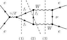
In addition to the -suppressed terms from the potential region of the one-loop diagrams shown in Figure 3, there is another NLO contribution from the leading terms of two-loop diagrams with one hard and one potential loop, which may also be associated with the Born cross section. An example is displayed in Figure 4. Cut (1) does not correspond to a four-fermion final state and must be dropped. Cut (3) corresponds to the interference of a tree-level production operator with the real part of a hard one-loop correction to a production operator. Since the -channel diagrams do not contribute to the leading-power production operator, this cut is beyond NLO. Cut (2) is a contribution to what is usually termed the “Born cross section” corresponding to the interference of single and double resonant diagrams in the kinematic region where both fermion pairs have invariant mass of order . The contribution from this cut is contained in the imaginary parts of the hard one-loop correction to the production operators. The threshold suppression of the -channel diagrams applies here as well, hence this contribution is also not relevant at NLO.
3.2 Decay-width correction for the flavour-specific cross section
As already noted, the expression (33) has to be modified in order to take the radiative correction to the decay correctly into account. In this subsection we derive the required modification of the formula, but note that it will not be needed for the comparison to the Born cross section, where radiative corrections are excluded.
To include the loop corrections to decay for the flavour-specific four-fermion final state we have to identify contributions to the forward-scattering amplitude from cut two-loop self-energy insertions and include only the appropriate cuts containing a muon and muon-antineutrino or up and anti-down quarks and, possibly, a photon. Repeating the expansion in the potential region performed in Section 3.1 for the cut diagram with flavour-specific cuts selected, one finds that in the pole mass renormalization and on-shell field renormalization scheme adopted here all terms in the expansion are correctly treated by multiplying the totally inclusive result by the ratio of leading-order partial branching fractions, , except for one term involving the insertion of . In (33) this insertion results in part of the term involving , and is also multiplied by . We therefore have to modify this term to include the flavour-specific cuts correctly. At NLO we have to consider diagrams where is inserted in only one of the two -lines. Cutting this line produces a contribution to the imaginary part of the forward-scattering amplitude of the form
| (34) |
where is the inverse propagator of the non-relativistic boson. The first two terms correspond to cutting the line to the left and right of the insertion. The flavour-specific final states are extracted from these cuts as discussed below (16). This amounts to multiplying the NLO correction (33) by the leading-order branching ratios, so these two terms are treated correctly by the factor . The last term corresponds to a cut two loop self-energy insertion, where only the cuts leading to the desired final state must be taken into account. Therefore here has to be replaced by and , respectively, to obtain the NLO cross section for the four-fermion final state. To implement these replacements, note that the contribution of the last term in (34) to the forward-scattering amplitude is of the form . We can therefore compensate the incorrect treatment of the flavour-specific cross section in (33) by subtracting this contribution for each line and adding the flavour-specific corrections. Multiplying by the leading-order branching fraction for the second line one obtains the additional NLO correction to the cross section,
| (35) |
At NLO this correction is equivalent to multiplying the imaginary part of the leading-order (or even next-to-leading order) forward-scattering amplitude by the one-loop corrected branching ratios rather than by , where . The NLO partial decay rates are calculated in Section 4.1.
3.3 Expansion in the hard region
We now consider the hard contributions, which determine the matching coefficients of four-electron production-decay operators. As already discussed in Section 2.2, the one-loop diagrams shown in Figure 3 do not provide imaginary parts of the forward-scattering amplitude. The leading hard contributions originate from the two-loop diagrams in Figure 5. These diagrams are to be calculated in standard perturbation theory with no width added to the propagator, but expanded near threshold. The result must be of order , which results in a N1/2LO correction relative to the leading-order cross section. Higher-order terms in the hard region come from higher-order terms in the expansion (in ) near threshold and from diagrams with more hard loops, all of which are N3/2LO and smaller.

In the hard region it is simpler to calculate the four-fermion cross section directly as the sum over the relevant cuts of the forward-scattering amplitude as shown in Figure 5. Note that this includes cutting lines as well as diagrams with self-energy insertions into the propagator. This can be interpreted as an expansion of the resummed propagator in the distribution sense [32, 33], such as
| (36) |
“PV” denoting the principal value. The left-hand side arises from cutting fermion-loop insertions into the propagator, but not the lines itself. But the leading term in the expansion of this expression, equivalent to the narrow-width approximation, looks as if a line with no self-energy insertions is cut.
The principal-value prescription is redundant at N1/2LO, where the singularity in the integrand is located at one of the integration limits, and is regularized by dimensional regularization, which has to be supplied in any case to regulate infrared divergences that arise as a consequence of factorizing hard and potential regions in the threshold expansion. As in the potential region, the integrals are actually analytically continued to finite values, since the divergences are odd power divergences. The result of the calculation can be written as
| (37) |
Here the first sum extends over the diagrams as labelled in Figure 5, the second over the fermions in the internal fermion loops. The explicit values of the coefficients arising from the diagrams h1-h3 are
| (38) |
The three coefficients contain the contribution of the diagrams h1-h3 shown in Figure 5 and of the symmetric diagrams with self-energy insertions on the lower line. contains also the contribution of the complex conjugate of h2. The explicit expressions of coefficients and , with , for the diagrams h4-h7 are given in Appendix A. Similar to (32) the -dependence of the arises trivially from photon and propagators, and we could put at N1/2LO. Since all other terms in (37) are energy-independent, we conclude that the leading hard contribution results in a constant N1/2LO shift of the cross section.
This contribution can be interpreted as arising from a final state where one fermion pair originates from a nearly on-shell decay, while the other is produced non-resonantly, either from a highly virtual , or as in the truly single-resonant diagrams h4-h7. Numerical investigation reveals that the contribution from h4-h7 is rather small, below of the full tree cross section in the energy range GeV and GeV. Below GeV it becomes negative and its magnitude grows to at GeV. The smallness of the single-resonant contributions is in part due to large cancellations between the diagrams h4 and h5.
The comparison with the Born cross section performed below shows that the region of validity of the EFT expansion is significantly enlarged, if the energy-dependent N3/2LO terms are included. These can only arise from the next-to-leading order terms of the expansion in the hard region (the expansion in the potential region produces only integer-power corrections in ). The energy-dependent terms are related to the next order in the threshold expansion of the cut diagrams in Figure 5. The computation for the numerically dominant diagrams h1-h3 gives
| (39) |
where
| (40) |
Other N3/2LO corrections related to the Born cross section arise from cut three-loop diagrams of the type h1-h3, but with two self-energy insertions, and of type h4-h7 with one insertion. This N3/2LO term is (almost) energy-independent and can be parameterized by
| (41) |
The coefficients are equal to the factors multiplying in (39) and we omitted the small contributions from h4-h7. The calculation of the numerical coefficients is non-trivial, since it contains products of distributions. A rough estimate of these corrections is , resulting in an energy-independent contribution to the cross section of order . The comparison below suggests that actually it is significantly smaller.
3.4 Comparison to the four-fermion Born cross section
We compare the successive EFT approximations to the four-fermion Born cross section in the fixed-width scheme. We discuss only the unpolarized cross section given by . The relevant terms are given in (17), (33), (37), and (39). The input parameters are taken to be
| (42) |
The pole mass is related to the on-shell mass through the relation (valid to )
| (43) |
where
| (44) |
We use the fine-structure constant in the scheme, , and the on-shell Weinberg angle . Inserting (44) into (43), and solving the equation for , we get the following pole parameters:
| (45) |
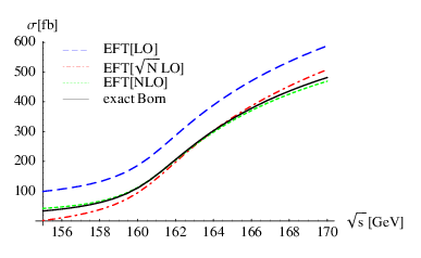
The value of the width used here is the leading-order decay width (19), excluding the one-loop QCD correction. This is appropriate for a tree-level calculation and ensures that the branching ratios add up to one. Correspondingly we set in the effective-theory calculation. In Figure 6 we plot the numerical result obtained with Whizard [17] for the tree-level cross-section, and the successive effective-theory approximations. We used the fixed-width scheme in Whizard and checked that the results from the O’Mega [34], CompHep [18] and MadGraph [20] matrix elements agree within the numerical error of the Monte-Carlo integration. The large constant shift of about 100 fb by the N1/2LO correction from the hard region is clearly visible, but the NLO approximation is already close to the full Born calculation. In Table 1 we perform a more detailed numerical comparison, now including also the N3/2LO approximation. (The missing energy-independent N3/2LO terms are set to zero.) We observe that the convergence of the expansion is very good close to the threshold at GeV, as should be expected. The accuracy of the approximation degrades as one moves away from threshold, particularly below threshold, where the doubly-resonant potential configurations are kinematically suppressed. If one aims at accuracy of the cross section, the NLO approximation suffices only in a rather narrow region around threshold. Including the N3/2LO term from the first correction in the expansion in the hard region leads to a clear improvement both above ( at 170 GeV) and below threshold ( at 155 GeV). The energy region where the target accuracy is met now covers the region of interest for the mass determination (see Section 6.4).
| (fb) | |||||
|---|---|---|---|---|---|
| EFT(LO) | EFT(LO) | EFT(NLO) | EFT(LO) | exact Born | |
| 155 | 101.61 | 1.62 | 43.28 | 31.30 | 34.43(1) |
| 158 | 135.43 | 39.23 | 67.78 | 62.50 | 63.39(2) |
| 161 | 240.85 | 148.44 | 160.45 | 160.89 | 160.62(6) |
| 164 | 406.8 | 318.1 | 313.5 | 318.8 | 318.3(1) |
| 167 | 527.8 | 442.7 | 420.4 | 429.7 | 428.6(2) |
| 170 | 615.5 | 533.9 | 492.9 | 505.4 | 505.1(2) |
4 Radiative corrections
In this section we calculate the NLO contributions that correspond to genuine loop corrections to four-fermion production. As outlined in Section 2.3 there are several such contributions: an electroweak correction to the matching coefficient of the leading pair-production operator and to decay; a correction from potential photons associated with the Coulomb force between the slowly moving bosons; and soft and collinear photon effects.
4.1 Hard corrections to production and decay
The two hard electroweak corrections required for a NLO calculation are the one-loop corrections and in the production operator (23) and the two-loop electroweak self-energy , see (21). We reiterate that these are conventional perturbative calculations performed in a strict expansion in . In particular, in the ’t Hooft-Feynman gauge, the propagators of the massive gauge bosons are simply given by and the self-energy insertions are taken into account perturbatively. All fermions except for the top quark are treated as massless.
Before addressing these two calculations separately, we briefly discuss the renormalization conventions for the parameters and fields of the electroweak standard model (SM). For a scattering amplitude, whose tree-level expression is proportional to the one-loop counterterm is given by
| (46) |
where the sum extends over all external lines. As specified in (42) the three independent parameters of the electroweak SM are taken to be the and boson mass, and the Fermi constant (including the electromagnetic correction to muon decay in the Fermi theory), while and are derived quantities. Similar to the scheme, the -scheme for defining the electromagnetic coupling has the advantage that the light-fermion masses can be set to zero [35, 36]. The counterterm for is related to the - and -boson self-energies. In the scheme we have
| (47) |
where is the transverse self-energy of the boson66 6 In the conventions used here and in [13] the sum of the amputated 1PI graphs is given by which is the opposite sign compared to [36]. and
| (48) |
appears in the explicit expression for the electroweak correction to muon decay, (see e.g. [36]). For the field-renormalization counterterms for the external lines we use the conventional on-shell scheme for wave-function renormalization [36] in accordance with the choice made in Section 3.1 for the renormalized propagator. In particular, for the -boson and fermion wave-function renormalization we have
| (49) |
where denotes the self energy of the fermion. (Note that .) The on-shell field renormalization of the fermions ensures that no further finite renormalization is needed in calculating the scattering amplitude. On the other hand, since we never consider a physical process with external bosons, the renormalization factor for the field is purely conventional, and our final result is independent of the convention for . However, the matching coefficient of the production operator calculated below does depend on this convention. The dependence is cancelled by the dependence of (28) on , the on-shell derivative of the renormalized one-loop self-energy, whose value depends on .
4.1.1 Production vertices
The general method on how to obtain the matching equations needed to determine the short-distance coefficients of production operators has been discussed in [13]. For and we compute the scattering amplitude at leading order in the non-relativistic approximation using dimensional regularization in dimensions. This is compared to the amplitude obtained with the tree-level operator in the effective theory and the matching coefficient is determined to make the results agree. The matching coefficients thus determined are gauge invariant by construction provided the scattering amplitude is calculated with the external boson momenta at the complex pole position. The matching prescription also includes an additional factor [13], as given in (12), for each external field. However, here we depart from the “correct” matching procedure and omit the factor , since it was already included in Section 3.1 (see discussion after (28)).

The diagrams for the scattering process are generated with FeynArts [37] and the algebra is performed with FeynCalc [38]. At one loop, there are 65 two-point diagrams, 84 three-point diagrams and 31 four-point diagrams (generically counting up-type quarks, down type quarks, leptons and neutrinos), some of which are shown in Figure 7. Due to the simplified kinematics, many of these diagrams do not contribute. In fact, since the one-loop contributions are already suppressed by it is sufficient to take the leading order in the non-relativistic expansion of the one-loop diagrams and to set , to rather than to the complex pole position. Thus, for the momenta we use whereas the incoming lepton momenta can be parametrized as and with . This results in two simplifications. First, many diagrams vanish consistent with the fact that the tree-level -channel diagrams do not contribute at leading order in the non-relativistic expansion. Second, the number of scales present in the loop integrals is reduced. Due to the simplified kinematics, all box integrals can be reduced to triangle diagrams and the one-loop correction to the amplitude for the process takes the simple form
| (50) |
expected from (23), with denoting the polarization vectors of the bosons. (For , the fermion helicities are reversed.) The scalar coefficients can be obtained by projections of the full amplitude. Thus, we are left with the calculation of a scalar quantity and standard techniques for the reduction of tensor and scalar integrals can be applied.
In the computation of all poles cancel and we are left with a finite result. This is to be expected, since the corresponding Born term vanishes, as indicated in (13). For , the matching coefficient of the operator that does not vanish at tree level, the poles do not cancel. After adding the counterterm (46) with , it takes the form
| (51) |
where the finite part together with the expression for is given explicitly in Appendix B. For the final expression of the matching coefficient, the poles have to be subtracted. However, we leave them explicit in order to demonstrate their cancellation against (double) poles from the soft contribution and poles related to initial-state collinear singularities. Numerically,
| (52) |
for GeV, GeV, top-quark mass GeV and Higgs mass GeV.
The matching coefficients and both have a non-vanishing imaginary part. Taken at face value, this imaginary part contributes to the imaginary part of the forward scattering amplitude and, therefore, to the total cross section. Denoting by the NLO contribution to resulting from we have
| (53) |
However, the second term in (53) is induced by cuts that do not correspond to the final state we are interested in, such as the intermediate state in the fourth diagram of Figure 7. In fact, at leading order in the non-relativistic expansion, none of the diagrams that contribute to the hard matching coefficients contains either a quark or a muon. To obtain the flavour-specific cross section we are concerned with, we therefore have to drop the second term in (53) and in what follows it is always understood that we take the real part of the matching coefficients and . Recalling the discussion of cut (2) at the end of Section 3.1, we note that beyond NLO the situation is more complicated, as some of the cuts contributing to the imaginary part of the matching coefficient do correspond to the flavour-specific cross section we are interested in.
The contribution to the cross section resulting from the NLO correction to the production operators is obtained by multiplying the imaginary part of by the leading order branching ratios. The correction to the cross section for the polarization is therefore given by
| (54) |
Because there is no interference of the helicities and , the coefficient does not contribute at NLO. Introducing the abbreviations
| (55) |
for the non-relativistic propagators in the leading-order diagram, Figure 2, and , we can rewrite (54) as
| (56) | |||||
The unintegrated form of the result is given to make the cancellation of the -poles against other contributions computed in the following subsections more transparent.
4.1.2 Decay corrections
Next we discuss the electroweak correction to the matching coefficient . In the pole mass and on-shell field renormalization scheme . The cuts of the 2-loop electroweak self-energy consist of two parts, corresponding to the virtual and real hard corrections to the pole decay width. Dealing with the total cross section, we only need the sum of these two. However, we also have to discuss how to obtain results for the flavour-specific process . To aid this, we will discuss the virtual and real corrections separately, starting with the former.
The virtual one-loop correction to the pole-scheme decay width into a single lepton or quark doublet can be written as
| (57) |
where the tree-level widths in dimensions are and . The calculation of involves the evaluation of the diagrams depicted in Figure 8 with obvious modifications for the leptonic decay. After adding the counterterm (46) with we obtain
| (58) |
where for the leptonic (hadronic) decay we have to set the electric charges to ( ). The finite parts of the matching coefficients are given explicitly in Appendix B. Numerically,
| (59) |
for GeV, GeV, GeV, and GeV.

To this we have to add the correction due to hard real radiation of a single photon. Since the corresponding soft corrections vanish, the hard real corrections are equivalent to the real corrections evaluated in the standard electroweak theory and their calculation is straightforward. We compute the bremsstrahlung diagrams and integrate the squared amplitude (divided by ) over the -dimensional phase-space [39]. The expression thus obtained contains infrared (double) poles which cancel the poles in (57) and we are left with finite expressions for the flavour-specific leptonic and hadronic matching coefficients. Including the (two-loop) QCD correction to the hadronic decay, they read
| (60) |
Strictly speaking, for the computation of these matching coefficients we have to expand around the complex pole and not around . However, the difference in the width is of order and thus beyond NLO [2].
4.2 Coulomb corrections

The exchange of potential photons with energy and three-momentum , shown in Figure 9, corresponds to insertions of the non-local four-boson interactions in the effective Lagrangian (11). These insertions can be summed to all orders in terms of the Green function of the Schrödinger operator evaluated at . Using the representation of the Green function given in [40], we obtain [41]
| (61) |
where is Euler’s psi-function, and a subtraction-scheme dependent real constant that drops out in the cross section has been omitted. The diagram with no photon exchange is not included in this expression, since it corresponds to the leading-order amplitude (15). The logarithm constitutes a correction relative to the leading-order scattering amplitude (15). The expansion of the psi-function in results in an expansion in powers of . Thus, the Coulomb correction up to NLO reads
| (62) |
This contributes only to the LR helicity cross section, since the production operator at the vertices in Figure 9 is the leading order one (13). Directly at threshold () the one-photon exchange N1/2LO term (the logarithm in (62)) is of order 5% relative to the leading order. Two-photon exchange is only a few-permille correction, confirming the expectation that Coulomb exchanges do not have to be summed to all orders due to the large width of the boson. The one and two Coulomb-exchange terms have already been discussed in [10, 11].
4.3 Soft-photon corrections
We now turn to the radiative correction originating from soft-photon exchange. These are contributions to the forward-scattering amplitude, and correspond to two-loop diagrams in the effective theory containing a photon with momentum components . The relevant Feynman rules are given by the coupling of the soft photon to the fields in the PNRQED Lagrangian (11) and to the collinear electrons and positrons contained in the SCET Lagrangian. The latter is simply the eikonal coupling , where is the direction of the four-momentum of the electron or positron. The topologies contributing to the two-loop forward-scattering amplitude are shown in Figure 10. The -boson vertices are leading-order production vertices, hence at NLO the soft correction applies only to the left-right helicity forward-scattering amplitude. Note that (mm2) is not a double-counting of the Coulomb-exchange diagram in Figure 9, since the two diagrams refer to different loop momentum regions.

It is well known that for the process the soft-photon corrections related to the final state cancel for the inclusive cross section [42, 43]. The diagrams of type (im) in Figure 10 cancel pairwise when the sum over incoming positrons and electrons is performed. The sum of the diagrams of the form of (mm1) and (mm2) cancels after the loop integrals are performed. Therefore the sum of all diagrams where a soft photon couples to an line vanishes. In the effective theory this cancellation can be seen from the outset, since it follows from the particular form of the leading coupling of a soft photon to non-relativistic bosons in the effective Lagrangian (11), which involves only . Since the residual gauge invariance of the effective Lagrangian allows one to set the time-like component of the photon field to zero, at leading order the couplings can be removed from the Lagrangian.
Therefore the soft-photon correction in the effective theory is given by the initial-initial state interference diagrams. However, diagram (ii2) leads to a scaleless integral which vanishes in dimensional regularization, and diagram (ii3) and the symmetric diagram are proportional to and , respectively. The only non-zero diagram is (ii1) and the corresponding crossed diagram. The sum of the two diagrams evaluates to
| (63) | |||||
The double -pole in (63) cancels against the pole in the hard matching coefficient; the single pole can be factorized into the initial-state electron (positron) structure function as shown in Section 5. Subtracting the pole part of the integrand (63) before performing the integration, one obtains
| (64) |
As before, the integration has been performed by closing the integration contour in the upper half-plane and picking up the pole at . Because of the absence of soft corrections related to the final state, at NLO the soft corrections to the flavour-specific process (1) can be obtained by multiplying the soft two-loop contributions to the forward-scattering amplitude by the leading-order branching ratios, thus
| (65) |
As a check, we also calculated the soft corrections directly for the process (1) and found agreement with the simpler calculation of the forward-scattering amplitude.
4.4 Collinear-photon corrections

Finally we consider collinear-photon corrections, corresponding to photon energies of order , and photon virtuality of order . The four-momentum of the photon is proportional to the initial-state electron or positron momentum. The collinear photon couplings arise from the SCET Lagrangian, while their couplings to the bosons is encoded in the collinear Wilson lines in the production operators. The diagrams corresponding to NLO contributions are shown in Figure 11. As discussed in [13] all these diagrams are scaleless for on-shell, massless initial-state particles. However, we shall have to say more about collinear effects in Section 5, when we include the resummation of large initial-state radiation logarithms.
4.5 Summary of radiative corrections
The radiative correction to the next-to-leading order cross section is given by the sum of the corrections (56), (65), (62), (35) computed in the previous sections,
| (66) |
Recall that this refers to the helicity initial state, while there are no radiative corrections to the other helicity combinations at NLO. The radiative correction to the unpolarized cross section is one fourth of the LR contribution.
Because of the approximation , the cross section is not infrared-safe, as can be seen by summing the four contributions. The Coulomb and decay corrections are free of infrared singularities. For the sum of the soft (63) and hard (56) terms we obtain the following expression:
| (67) | |||||
The cross section is a “partonic” cross section. It should be convoluted with the electron (positron) distribution function, which contains the infrared effects associated with the electron mass scale. In the following section we discuss how the partonic cross section is transformed to the infrared-finite physical cross section.
5 Initial-state radiation
The remaining -poles in (67) are associated with emission of photons collinear to the incoming electron or positron, and can be factorized into the electron distribution function , in terms of which the physical cross section reads [44, 45]
| (68) |
Here is our result for the NLO helicity-specific cross section after adding the Born cross section from Section 3 and the radiative correction from (66) with the infrared -poles minimally subtracted. The partonic cross section depends on the scales and the factorization scale . The electron distribution function in the scheme depends on and the very-long distance scale . The physical cross section is independent of and includes the electron-mass dependence up to effects suppressed by powers of . By evolving the electron distribution from the scale to the scale , one sums large collinear logarithms , with , from initial-state radiation of photons to all orders in perturbation theory. A NLO calculation of the partonic cross section should go along with a next-to-leading logarithmic approximation, where all terms with and are summed. Note that here we do not attempt to sum logarithms of , which are less important, although the effective-theory formalism is ideally suited for this summation as well.
Unfortunately the structure functions available in the literature do not correspond to the scheme and sum only leading logarithms . To convert our result to this scheme and sum the leading-logarithmic initial-state radiation effects we proceed as follows: first, using the expansion , we compute the scheme-independent NLO physical cross section without summation of collinear logarithms,
| (69) |
Then, by comparing this to the corresponding equation in the conventional scheme,
| (70) |
we determine , and hence . Finally, we calculate the initial-state radiation resummed cross section
| (71) |
in the conventional scheme for the electron (positron) distribution functions. Note that since the Born cross section for the RL helicity combination is already a NLO effect, the scheme conversion must be performed only for . For we simply have .
Step 1: Calculation of the fixed-order physical cross section .
Rather than calculating the last term on the right-hand side of (69), we compute directly the radiative correction to the physical cross section, , by converting , where the collinear divergences are regulated dimensionally, into the expression when the electron mass itself is used as the regulator.
In the presence of the new scale there are two new momentum regions that give non-zero contributions to the radiative corrections. They correspond to hard-collinear photon momentum (, ) and soft-collinear photons (, ).77 7 The existence of two collinear momentum regions is related to the fact that the pair-production threshold region probes the electron distribution function near , where hard-collinear real radiation is inhibited. The corresponding loop integrals are scaleless when ; for , they supply the difference
| (72) |
In other words is the sum of the four contributions in (66) plus those from the two new momentum regions.
Only a small subset of all the radiative correction diagrams has hard- or soft-collinear contributions, namely those containing a photon line connecting to an external electron or positron. The topology of the soft-collinear and hard-collinear diagrams is identical to the (ii) and (im) diagrams in Figure 10, and to the diagrams in Figure 11, respectively. The calculation is straightforward. In each region we simplify the integrand by neglecting all small terms, since the leading-order term in the expansion in each region is sufficient. The soft-collinear correction is
| (73) | |||||
the hard-collinear correction
| (74) | |||||
The structure of the logarithms makes it clear that the two contributions arise each from a single scale, and , respectively. Adding (66), (73), (74), and making use of (67) results in the factorization-scheme independent radiative correction to the physical cross section,
| (75) | |||||
After performing the -integral we may set to four and obtain a finite result. As expected the -poles have cancelled, but the infrared-sensitivity of the cross section is reflected in the large logarithms .
Step 2: Calculation of .
Comparing the right-hand sides of (69) and (70), we obtain the radiative correction to the conventional “partonic” cross section
| (76) |
where is the term in the expansion of the conventional electron structure function provided in [46, 47]. In the notation of [47] we employ the structure function with . To calculate the subtraction term in (76) it is sufficient to approximate in the expression for , to set to the leading-order Born term (17) with the replacement of by , and to use in the limit ,
| (77) |
We then reintroduce the integral over , and exchange the - and -integration to obtain
| (78) |
which shows that is free from the large electron mass logarithms. To obtain the final form in (78) we have shifted the integration variable to . Summing (75) and (78), and performing the -integration, gives the final result for the next-to-leading order radiative correction to the conventional “partonic” cross section
| (79) | |||||
Step 3: Computation of the resummed cross section.
The summation of collinear logarithms from initial-state radiation is completed by performing the convolution (71) using the Born cross section and the radiative correction (79) together with the electron structure functions from [46, 47]. This constitutes our final result, which we shall discuss in detail in the following section.
6 NLO four-fermion production cross section
We now present our NLO predictions for the total cross section of the process and assess the theoretical error on the -mass measurement due to the uncertainties in the cross-section calculation.
6.1 Input parameters and summation of -width corrections
In addition to the input parameters (42) used for the comparison of the tree cross section we use and the masses
| (80) |
We use the fine structure constant in the scheme everywhere including the initial-state radiation. With these input parameters we obtain from (60) the numerical value of the width to NLO,
| (81) |
Note that we have chosen to multiply not only the leading order, but also the electroweak correction to the hadronic decay by the factor defined in (20). In the numerical results below we will resum the full NLO width (81) in the effective-theory propagator (10), that is we do not perform an expansion of the propagator in the perturbative corrections to the matching coefficient . We now describe how the formula for the NLO cross section must be modified to accomplish this summation of the width corrections. Readers not interested in this technical detail may move directly to the next subsection.
Leaving unexpanded amounts to setting to zero in the NLO tree cross section (33) and to replacing by wherever it appears. Some care has then to be taken in order to obtain the correct cross section for the flavour-specific four-fermion final state from the calculation of the forward-scattering amplitude. Cutting the effective-theory propagator leads to a factor
| (82) |
analogously to (16). In the direct calculation of the four-fermion production cross section the numerator arises from integrating over the two-body decay phase space, which yields the leading-order partial width. Hence, we have to multiply all contributions to the forward-scattering amplitude with two cut effective-theory propagators (the potential contributions in Section 3.1, the Coulomb and soft radiative corrections, and the contribution from the one-loop correction to the production operator) by a factor instead of the factor used in the tree level analysis. In the calculation of the matching coefficient of the four-electron production-decay operator performed in Section 3.3 the self-energy insertions on one of the two lines are treated perturbatively, and the decay subprocess is already correctly included at lowest order, while the other is effectively treated in the narrow-width approximation
| (83) |
To obtain the correct flavour-specific final state we therefore have to include a single prefactor or , depending on the charge. As shown in Table 2, with these prescriptions the N3/2LO effective-theory approximation and the full Born cross section (in the fixed-width definition now using (81)) are again in very good agreement, similar to the earlier comparison, where only was resummed in the propagator.
| (fb) | |||
|---|---|---|---|
| EFT Tree (NLO) | EFT Tree (N3/2LO) | exact Born | |
| 155 | 42.25 | 30.54 | 33.58(1) |
| 158 | 65.99 | 60.83 | 61.67(2) |
| 161 | 154.02 | 154.44 | 154.19(6) |
| 164 | 298.6 | 303.7 | 303.0(1) |
| 167 | 400.3 | 409.3 | 408.8(2) |
| 170 | 469.4 | 481.7 | 481.7(2) |
As already mentioned the electroweak radiative corrections are correctly treated by multiplying the inclusive forward-scattering amplitude by , except for the correction to decay itself. These contributions are included by adding the decay correction
| (84) |
instead of (35). The QCD corrections up to order are included in a similar way. Because of the large NLO corrections to the tree cross section and the large effect of ISR, it is sensible to apply the QCD decay correction to the full NLO electroweak cross section. This amounts to multiplying , by the radiative correction factor as given in (20), wherever they appear, which is consistent with the definition of the NLO width (81). If in addition we also account (approximately) for the QCD decay correction to the non-resonant contributions from Section 3.3, this is equivalent to multiplying the entire NLO electroweak cross section by and using the QCD corrected width (81) as will be done in the following analysis.
6.2 NLO four-fermion production cross section in the effective theory
The convolution of the “partonic” cross section with the electron structure functions contains integrations over partonic center-of-mass energies far below threshold, where the effective field theory approximation is not valid. The EFT calculation should be matched to a full cross section calculation below some cms energy, say GeV, where for the full calculation a Born treatment is sufficient, because the cross section below threshold is small. Since the N3/2LO EFT approximation to the Born cross section provides a very good approximation (except significantly below threshold), we have found it more convenient to replace the EFT approximation to the Born cross section convoluted according to (71) by the full ISR-improved Born cross section as generated by the Whizard program [17] rather than to perform this matching. To this we add the NLO radiative correction (79) (replacing the leading-order cross section by the full Born cross section in the decay correction (84)), which we also convolute with the electron distribution functions. Here we simply cut off the integration region GeV. The dependence on this cut-off is negligible. Lowering it from to GeV to GeV ( GeV), changes the cross section at GeV from fb to fb (fb), while the dependence on the cut-off for higher cms energy is even smaller.
| (fb) | ||||
|---|---|---|---|---|
| Born | Born(ISR) | NLO | NLO(ISR-tree) | |
| 158 | 61.67(2) | 45.64(2) | 49.19(2) | 50.02(2) |
| [-26.0%] | [-20.2%] | [-18.9%] | ||
| 161 | 154.19(6) | 108.60(4) | 117.81(5) | 120.00(5) |
| [-29.6%] | [-23.6%] | [-22.2%] | ||
| 164 | 303.0(1) | 219.7(1) | 234.9(1) | 236.8(1) |
| [-27.5%] | [-22.5%] | [-21.8%] | ||
| 167 | 408.8(2) | 310.2(1) | 328.2(1) | 329.1(1) |
| [-24.1%] | [-19.7%] | [-19.5%] | ||
| 170 | 481.7(2) | 378.4(2) | 398.0(2) | 398.3(2) |
| [-21.4%] | [-17.4%] | [-17.3%] | ||
Our result for the NLO four-fermion cross section is shown in Table 3. The impact of radiative corrections is seen by comparing the exact Born cross section (second column, identical to the last column in Table 2), the ISR-improved Born cross section (third column) and the NLO result (fourth column). As is well-known initial-state radiation results in a large negative correction (about 25%). The size of the genuine radiative correction is best assessed by comparing the “NLO” column to the “Born(ISR)” column and thus seen to be about . Given that we aim at a theoretical accuracy at the sub-percent level, this is an important effect. We shall discuss below, in Section 6.4, an estimate of the remaining uncertainty of the NLO cross section.
One uncertainty is related to the fact that the conventional implementation of ISR sums only leading logarithms, whereas a NLO calculation of the partonic cross section should be accompanied by a next-to-leading logarithmic resummation. Thus rather than convoluting the full NLO partonic cross section with the structure functions as done above and indicated in (71), one could equally well convolute only the Born cross section, and add the radiative correction without ISR improvement, as done in some previous NLO calculations [6, 15]. Although we favour the first option, the two implementations are formally equivalent, because the difference is a next-to-leading logarithmic term. We therefore consider this difference as an estimate of the uncertainty induced by the missing next-to-leading logarithmic evolution of the structure functions. To assess this uncertainty, in the fifth column of Table 3 we show the NLO cross section based on the expression
| (85) |
where the NLO correction to the “partonic” cross section, , is given in (79) (with replaced by ). The comparison of the last and second-to-last columns of Table 3 shows that the difference between the two implementations of ISR reaches almost two percent at threshold and is therefore much larger than the target accuracy in the per-mille range. The difference between the two implementations becomes smaller at higher energies and is negligible at GeV. The impact of this difference on the accuracy of the -mass measurement will be investigated further in Section 6.4.
6.3 Comparison to the full four-fermion calculation
| (fb) | ||||
|---|---|---|---|---|
| Born | NLO(EFT) | ee4f [15] | DPA [15] | |
| 161 | 150.05(6) | 104.97(6) | 105.71(7) | 103.15(7) |
| 170 | 481.2(2) | 373.74(2) | 377.1(2) | 376.9(2) |
We now compare the NLO prediction of the four-fermion production process (1) obtained with the effective-theory method to the full NLO calculation performed in [15] in the complex mass scheme. For this comparison, we adjust our input parameters to those of [15],
| (86) |
and use in the relative radiative corrections as in [15]. We first compare the strict electroweak NLO calculation, i.e. the cross section without the QCD correction and without initial-state radiation beyond the first-order term. In the effective-theory calculation the corresponding radiative correction is given by (75) omitting the second-order Coulomb correction and the factor in the decay width. In Table 4 the EFT result and the result of [15] are shown in the columns labelled “NLO(EFT)” and “ee4f”, respectively. For comparison we also show the results for the Born cross section and in the double-pole approximation (“DPA”) in the implementation of [6] as quoted in [15]. The main observation is that the difference between the EFT and the full four-fermion calculation is only at GeV and grows to about at GeV.
Next, in Table 5, we compare to the full result including the QCD correction and the resummation of ISR corrections with [15]. Here we implement the QCD correction as in [15] by multiplying the entire electroweak NLO result by the overall factor . Furthermore, we include ISR corrections only to the Born cross section as in (85), in agreement with the treatment of [15]. Again the second-order Coulomb correction is set to zero, because [15] does not include any two-loop effects. As before, the Table shows the two NLO calculations, the Born cross section (now ISR improved) and the double-pole approximation. The discrepancy between the EFT calculation and the full four-fermion calculation is around at threshold. The EFT approximation is significantly better than the double-pole approximation directly at threshold, while at higher energies the quality of the DPA improves relative to the EFT approximation, since no threshold expansion is performed in the DPA.
6.4 Theoretical error of the determination
The mass will probably be determined by measuring the four-fermion production cross section at a few selected cms energies near the pair-production threshold. In this section we estimate the error on the mass from various sources of theoretical uncertainty. To this end we assume that measurements will be taken at , and at , and that the measured values coincide with our NLO calculation (labelled “NLO(EFT)” in Table 3) corresponding to the pole mass . We denote by the cross section values at the six cms energy points for any other theoretical calculation of four-fermion production as a function of the input mass , and determine the minimum of
| (87) |
For simplicity we assume that each point carries the same weight, so is an arbitrary constant of mass dimension . (We checked that a more realistic assignment does not lead to significantly different results.) The value of at which attains its minimum provides an estimate of the difference in the measured value of due to the different theoretical cross section inputs, and . For instance if is the ISR-improved Born cross section (labelled “Born(ISR)” in Table 3), we obtain MeV, which tells us that comparing measurements to a theoretical calculation without the genuine radiative corrections would result in a value of which is about 200 MeV too low. The NLO calculation is therefore crucial for an accurate determination. Next we attempt to estimate whether it is accurate enough.
Treatment of initial-state radiation.
A look at the last two columns of Table 3 reveals that two different implementation of ISR, which are formally equivalent at the leading-logarithmic level, can lead to differences in the predicted cross section of at GeV, where the sensitivity to is largest. We take this as a measure for the uncertainty caused by the missing next-to-leading logarithmic corrections to the structure function. To estimate the error on caused by this uncertainty, we apply the procedure discussed above and find
| (88) |
This large error could be avoided by measuring the cross section predominantly around GeV rather than around GeV, but the sensitivity to is significantly smaller at higher energies (see Figure 12 below). Thus, this error should be eliminated by a consistent treatment of the electron structure functions at the next-to-leading logarithmic level, in which all NLL corrections are taken into account by convoluting the NLO cross section with the NLL structure functions. A related effect concerns the choice of scheme and scale of the electromagnetic coupling. The difference in the cross section between using and in the -scheme in the radiative correction (including, in particular, initial-state radiation) is about , which translates into another error of about MeV in the mass. The scale ambiguity of the coupling used in initial-state radiation can be resolved only in the context of a next-to-leading logarithmic resummation which takes the evolution of between and into account. On the other hand, the typical scales in the short-distance cross section are at least GeV, so that in the scheme is more appropriate than the low-energy electromagnetic coupling in the radiative correction to the short-distance cross section, since it is numerically close to the running coupling at GeV.
Uncalculated corrections to the “partonic” cross section.
The leading missing higher-order terms in the expansion in and are LO corrections to the forward-scattering amplitude from four-loop potential diagrams (third Coulomb correction), three-loop diagrams with two potential loops and one soft loop (interference of single-Coulomb and soft radiative corrections), two-loop potential diagrams with matching coefficients or higher-dimensional production operators, and the correction to the matching coefficients of the four-electron production-decay operators. The latter is expected to be the largest of these contributions, in particular since the non-resonant N1/2LO contributions are large at the Born level ( at threshold, see Table 1). Presumably, this contribution is also the origin of the difference between the EFT result “NLO(EFT)” and the full four-fermion calculation “ee4f” at GeV in Table 5. A rough estimate of this correction to the helicity-averaged cross section is
| (89) |
where is an -independent constant of order 1. (In fact, if we attributed the difference between our calculation (“NLO(EFT)”) and that of [15] (“ee4f”) at GeV exclusively to this contribution, we would obtain .) Thus, we choose , add (89) to the “NLO(EFT)” calculation, and minimize the function. From this we obtain an error
| (90) |
The second largest uncalculated correction to the partonic cross section is expected to come from diagrams with single-Coulomb exchange and a soft photon or a hard correction to the production vertex. A naive estimate of the sum of the two terms is
| (91) |
where the quantities involved have been defined in Section 4. Estimating the corresponding uncertainty on the mass as before, we find
| (92) |
Adding the two errors we conclude that the uncertainty on due to uncalculated higher-order effects in the effective field theory method is about MeV. Thus, to reach a total error of requires the inclusion of at least some LO corrections in the EFT approach. The larger of the two errors estimated above, due to the electroweak correction to production-decay operator, can be removed by using the full NLO four-fermion calculation, where this correction is included.

Summary.
The discussion above is summarized in Figure 12, where we plot for different values of as function of the cms energy, being our NLO result, “NLO(EFT)”. The relative change in the cross section is shown as dashed lines for . The shape of these curves shows that the sensitivity of the cross section to the mass is largest around the nominal threshold GeV, as expected, and rapidly decreases for larger . (The loss in sensitivity is partially compensated by a larger cross section, implying smaller statistical errors of the anticipated experimental data.)
The dark-shaded area in Figure 12 corresponds to the uncertainty on the cross section from (91), while the light-shaded area adds (linearly) the uncertainty from (89). The theoretical error decreases with , since in (89) is roughly energy-independent, while increases. The largest current uncertainty is, however, due to ambiguities in the implementation of ISR. The solid (red) curve gives the ratio of the two different implementations of ISR, NLO(EFT) vs. NLO(ISR-tree), both evaluated at . As mentioned above, we do not consider this as a fundamental problem, since this uncertainty can be removed with further work on a next-to-leading-logarithmic ISR resummation that will be required for many other processes at a high-energy collider as well.
7 Conclusion
We performed a dedicated study of four-fermion production near the pair-production threshold in view of the importance of this process for an accurate determination of the -boson mass. Our theoretical study of radiative and finite-width corrections was motivated by a corresponding experimental study [3] which showed that the planned high-luminosity linear collider might allow a measurement of with an error of only MeV from the threshold region. Our calculation, and the good agreement with the full NLO four-fermion cross section calculation of [15], demonstrates that accurate theoretical calculations are feasible and available in the threshold region. With regard to the mass determination, we find:
- •
A resummation of next-to-leading collinear logarithms from initial-state radiation is mandatory to reduce the error on below the 30 MeV level.
- •
The NLO partonic cross-section calculation in the effective theory approach implies a residual error of about 10 – 15 MeV on . The largest missing N3/2LO effect is probably due to the electroweak correction to the (non-resonant) production-decay vertex, which is included in the full NLO four-fermion calculation, and can thus be eliminated.
It is forseeable that both items can be removed, so we conclude that there is no fundamental difficulty in reducing the theoretical error in the mass determination from the threshold region to about 5 MeV.
The calculation presented here is also the first NLO calculation of a realistic process in unstable-particle effective theory, since [12, 13] discussed the case of a single resonance in a gauged Yukawa model. Comparison of our results for four-fermion production with numerical integrations of the Born matrix elements and the radiative correction shows good convergence of the EFT expansion, and very good agreement once the first subleading term in each essential region (potential/resonant, hard/non-resonant) is included. The EFT approach provides a consistent treatment of finite-width effects that can in principle be extended systematically to higher orders. Our final results take the form of compact analytic formulae, which has to be compared to the numerical and technical challenges [15] of the full NLO four-fermion cross section calculation. However, it should be mentioned that our calculation is restricted to the inclusive cross section, while a more flexible treatment of the final-state phase space is obviously desirable. This requires either applying effective-theory methods to four-fermion production amplitudes rather than the forward-scattering amplitude, or the consideration of specific cuts such as corresponding to invariant-mass distributions that allow for a semi-inclusive treatment. Interesting developments in this direction have recently been reported for top-quark pair production [48].
Acknowledgement
This work is supported in part by the DFG Sonderforschungsbereich/Transregio 9 “Computergestützte Theoretische Teilchenphysik”, the DFG Graduiertenkolleg “Elementarteilchenphysik an der TeV-Skala”, and the European Community’s Marie-Curie Research Training Network under contract MRTN-CT-2006-035505 ‘Tools and Precision Calculations for Physics Discoveries at Colliders’.
Appendix A Coefficients of non-resonant contributions
In this appendix we list the explicit expressions of the remaining coefficients and in (37). The functions are known analytically, and contain all the -dependence of the cross section (except for the overall factor ). They are determined by the photon and propagators and electroweak couplings. In the limit of vanishing fermion masses the only helicity configurations contributing to the cross section are . The coefficients are -independent, and result from dimensionally regularized cut loop integrals. Typically the last integration is performed numerically, after the subtraction of the singular terms which are integrated analytically, though some analytic results can be obtained. The results given below contain the contribution of the diagrams h4-h7 in Figure 5 including their complex conjugates, except for cut h6, where the complex conjugate is the diagram itself, and cut h7, where the symmetric diagram is automatically taken into account by summing over the four flavours.
Only the configuration contributes to the cut diagram h4:
| (93) |
where and are the couplings of left-handed fermions to and . always denotes the charge of the particle (not the anti-particle) in units of the positron charge. For the cut diagram h5 we have
| (94) |
where and . In this case both left-handed and right-handed incoming fermions contribute (), but only left-handed internal fermions. The coefficients of h6 are
| (95) |
while for h7 we get
| (96) |
where and are the couplings to and of the particles in the same SU(2) doublet (i.e. and ).
Appendix B Hard one-loop coefficients
We give here the explicit analytic results for the hard one-loop coefficients appearing in Section 4.1.
B.1 Production vertices
The general production operator we are concerned with in this appendix reads
| (97) |
where is the hard matching coefficient and refers to the helicity of the incoming leptons ( or ). Starting with , the matching coefficient at tree level is equal to , as can be read off (13). At NLO we have
| (98) |
where is the coefficient in (23). Before renormalization the NLO short-distance coefficient reads
| (99) | |||||
where all functions appearing in the above expression, and , are known analytically and are supplied in Appendix B.3. The counterterms in the scheme are computed from (46) and are given by
| (100) | |||||
The full renormalized coefficient is obtained by adding bare result and counterterms
| (101) |
The poles of are given explicitly in (51) and cancel once one takes into account soft and initial-state collinear radiation.
B.2 Virtual corrections to decay
The decay of a boson is implemented in the effective theory analogous to the production [9]. There are decay operators with collinear fields describing the decay products of the non-relativistic vector boson. For the flavour-specific decays under consideration we have up to NLO
| (104) |
These operators would be needed for the calculation of the scattering amplitude in the effective theory. However, for the total cross section (or the forward scattering amplitude) the directions , of the decay products will be integrated over and, as indicated in (4), there is no need to introduce collinear fields , , and in the effective theory. The matching coefficients of the decay operators enter only indirectly through . The virtual correction to the decay width is related to the coefficient functions of the decay operators. Ignoring QCD corrections, at NLO we have
| (105) |
We give here the explicit results for the electroweak corrections. The unrenormalized one-loop correction to the leptonic decay vertex reads
| (106) | |||||
and the corresponding counterterms computed from (46) are
| (107) |
Similarly the NLO bare correction to the hadronic vertex is given by
| (108) | |||||
and the corresponding counterterms are
| (109) | |||||
B.3 Integrals and auxiliary functions
The results for the short-distance coefficients and their counterterms have been written such that all poles in are apparent and the remaining functions are finite. We give here their analytic expressions. As usual the scalar two- and three-point functions are defined by
| (110) |
and
| (111) |
is then defined as
| (112) |
The auxiliary function used in the expressions for the matching coefficients is related to the two-point function by
| (113) |
and satisfies . It is sufficient to give this function for the following special arguments:
| (114) | |||||
where we introduced . The explicit result for the derivative of the two-point function that is needed reads
| (115) | |||||
The analytic expressions of the finite three-point functions appearing in the results given in (99)–(109) can all be obtained from
| (116) | |||||||
| (117) | |||||||
| (118) | |||||||
| (119) | |||||||
| (120) | |||||||
| (121) | |||||||
where we introduced .
References
- [1] Particle Data Group, W. M. Yao et al., J. Phys. G33, 1 (2006).
- [2] A. Sirlin, Phys. Rev. Lett. 67, 2127 (1991).
- [3] G. Wilson, in 2nd ECFA/DESY Study, pp. 1498–1505, Desy LC note LC-PHSM-2001-009.
- [4] W. Beenakker, F. A. Berends and A. P. Chapovsky, Nucl. Phys. B548, 3 (1999), [hep-ph/9811481].
- [5] A. Denner, S. Dittmaier, M. Roth and D. Wackeroth, Phys. Lett. B475, 127 (2000), [hep-ph/9912261].
- [6] A. Denner, S. Dittmaier, M. Roth and D. Wackeroth, Nucl. Phys. B587, 67 (2000), [hep-ph/0006307].
- [7] S. Jadach, W. Placzek, M. Skrzypek, B. F. L. Ward and Z. Was, Phys. Rev. D65, 093010 (2002), [hep-ph/0007012].
- [8] S. Jadach, W. Placzek, M. Skrzypek, B. F. L. Ward and Z. Was, Comput. Phys. Commun. 140, 432 (2001), [hep-ph/0103163].
- [9] M. Beneke, N. Kauer, A. Signer and G. Zanderighi, Nucl. Phys. Proc. Suppl. 152, 162 (2006), [hep-ph/0411008].
- [10] V. S. Fadin, V. A. Khoze and A. D. Martin, Phys. Lett. B311, 311 (1993).
- [11] V. S. Fadin, V. A. Khoze, A. D. Martin and W. J. Stirling, Phys. Lett. B363, 112 (1995).
- [12] M. Beneke, A. P. Chapovsky, A. Signer and G. Zanderighi, Phys. Rev. Lett. 93, 011602 (2004), [hep-ph/0312331].
- [13] M. Beneke, A. P. Chapovsky, A. Signer and G. Zanderighi, Nucl. Phys. B686, 205 (2004), [hep-ph/0401002].
- [14] A. P. Chapovsky, V. A. Khoze, A. Signer and W. J. Stirling, Nucl. Phys. B621, 257 (2002), [hep-ph/0108190].
- [15] A. Denner, S. Dittmaier, M. Roth and L. H. Wieders, Phys. Lett. B612, 223 (2005), [hep-ph/0502063].
- [16] A. Denner, S. Dittmaier, M. Roth and L. H. Wieders, Nucl. Phys. B724, 247 (2005), [hep-ph/0505042].
- [17] W. Kilian, in 2nd ECFA/DESY Study, pp. 1924–1980, DESY LC-Note LC-TOOL-2001-039.
- [18] A. Pukhov et al., hep-ph/9908288.
- [19] CompHEP, E. Boos et al., Nucl. Instrum. Meth. A534, 250 (2004), [hep-ph/0403113].
- [20] T. Stelzer and W. F. Long, Comput. Phys. Commun. 81, 357 (1994), [hep-ph/9401258].
- [21] F. Maltoni and T. Stelzer, JHEP 02, 027 (2003), [hep-ph/0208156].
- [22] C. W. Bauer, S. Fleming, D. Pirjol and I. W. Stewart, Phys. Rev. D63, 114020 (2001), [hep-ph/0011336].
- [23] C. W. Bauer, D. Pirjol and I. W. Stewart, Phys. Rev. D65, 054022 (2002), [hep-ph/0109045].
- [24] M. Beneke, A. P. Chapovsky, M. Diehl and T. Feldmann, Nucl. Phys. B643, 431 (2002), [hep-ph/0206152].
- [25] A. H. Hoang and C. J. Reisser, Phys. Rev. D71, 074022 (2005), [hep-ph/0412258].
- [26] M. Beneke and V. A. Smirnov, Nucl. Phys. B522, 321 (1998), [hep-ph/9711391].
- [27] A. Pineda and J. Soto, Phys. Rev. D59, 016005 (1999), [hep-ph/9805424].
- [28] M. J. G. Veltman, Physica 29, 186 (1963).
- [29] K. G. Chetyrkin, J. H. Kühn and A. Kwiatkowski, Phys. Rept. 277, 189 (1996), [hep-ph/9503396].
- [30] A. Aeppli, G. J. van Oldenborgh and D. Wyler, Nucl. Phys. B428, 126 (1994), [hep-ph/9312212].
- [31] R. G. Stuart, Phys. Lett. B262, 113 (1991).
- [32] F. V. Tkachov, hep-ph/9802307.
- [33] M. L. Nekrasov, Phys. Lett. B545, 119 (2002), [hep-ph/0207215].
- [34] M. Moretti, T. Ohl and J. Reuter, in 2nd ECFA/DESY Study, pp. 1981–2009, [hep-ph/0102195], DESY LC-Note LC-TOOL-2001-040.
- [35] S. Dittmaier and M. Krämer, Phys. Rev. D65, 073007 (2002), [hep-ph/0109062].
- [36] A. Denner, Fortschr. Phys. 41, 307 (1993).
- [37] T. Hahn, Comput. Phys. Commun. 140, 418 (2001), [hep-ph/0012260].
- [38] R. Mertig, M. Böhm and A. Denner, Comput. Phys. Commun. 64, 345 (1991).
- [39] W. J. Marciano, Phys. Rev. D12, 3861 (1975).
- [40] E. H. Wichmann and C. H. Woo, J. Math. Phys. 2, 178 (1961).
- [41] M. Beneke, in: Proceedings of the 8th International Symposium on Heavy Flavor Physics (Heavy Flavors 8), Southampton, England, 25-29 Jul 1999, [hep-ph/9911490].
- [42] V. S. Fadin, V. A. Khoze and A. D. Martin, Phys. Rev. D49, 2247 (1994).
- [43] K. Melnikov and O. I. Yakovlev, Phys. Lett. B324, 217 (1994), [hep-ph/9302311].
- [44] E. A. Kuraev and V. S. Fadin, Sov. J. Nucl. Phys. 41, 466 (1985).
- [45] W. Beenakker and A. Denner, Int. J. Mod. Phys. A9, 4837 (1994).
- [46] M. Skrzypek, Acta Phys. Polon. B23, 135 (1992).
- [47] W. Beenakker et al., in Physics at LEP2, Vol. 1, edited by G. Altarelli, T. Sjostrand and F. Zwirner, p. 79, 1996, [hep-ph/9602351], report CERN-96-01.
- [48] S. Fleming, A. H. Hoang, S. Mantry and I. W. Stewart, hep-ph/0703207.