Local Properties of $J$ -complex Curves
in Lipschitz-Continuous Structures

S. Ivashkovich, V. Shevchishin Address: Université de Lille-1, UFR de Mathématiques, 59655 Villeneuve d’Ascq, France. Email address: ivachkov@math.univ-lille1.fr Address: IAPMM Nat. Acad. Sci. Ukraine Lviv, Naukova 3b, 79601 Ukraine. Address: Department of Mathematics, University of Hamburg, Bundesstrasse 55, D-20146 Hamburg, Germany. Email address: shevchishin@googlemail.com

Date: August 11, 2026

Abstract.

We prove the existence of primitive curves and positivity of intersections of $J$ -complex curves for Lipschitz-continuous almost complex structures. These results are deduced from the Comparison Theorem for $J$ -holomorphic maps in Lipschitz structures, previously known for $J$ of class ${\mathcal{C}}^{1,Lip}$ . We also give the optimal regularity of curves in Lipschitz structures. It occurs to be ${\mathcal{C}}^{1,LnLip}$ , i.e., the first derivatives of a $J$ -complex curve for Lipschitz $J$ are Log-Lipschitz-continuous. A simple example that nothing better can be achieved is given. Further we prove the Genus Formula for $J$ -complex curves and determine their principal Puiseux exponents (all this for Lipschitz-continuous $J$ -s).

Key words and phrases:

Almost complex structure, pseudoholomorphic curve, cusp, Genus Formula, Puiseux exponents.

1991 Mathematics Subject Classification

Primary 32Q65, Secondary 14H50

1. Introduction

An almost complex structure on a real manifold $X$ is a section of ${\mathsf{End}}^{\mathstrut}_{\mathbb{R}}{TX}$ such that $J^{2}=-{\mathsf{Id}}$ . In this paper we are interested in the case when $J$ is Lipschitz-continuous. A $J$ -holomorphic curve in an almost complex manifold $(X,J)$ is a ${\mathcal{C}}^{1}$ -map $u:S\to X$ from a complex curve $(S,j)$ to $X$ such that $du$ commutes with complex structures, i.e., for every $s\in S$ one has the equality

du(s)\circ j(s)=J(u(s))\circ du(s)

of mappings $T_{s}S\to T_{u(s)}X$ . In a local $j$ -holomorphic coordinate $z=x+iy$ on $S$ and local coordinates $u=(u_{1},...,u_{2n})$ on $X$ this writes as

\frac{\partial u}{\partial x}+J(u)\frac{\partial u}{\partial y}=0,

(1.1)

i.e., as the Cauchy-Riemann equation.

The goal of this paper is to prove that $J$ -complex curves for Lipschitz-continuous $J$ possess all nice properties of the usual complex curves.

1.1. Existence of primitive parameterizations

Recall (see also Definition 4.2) that a $J$ -holomorphic map $u:S\to X$ is called primitive if there are no disjoint non-empty open sets $U_{1},U_{2}$ in $S$ that $u(U_{1})=u(U_{2})$ . Our first result states that every non-primitive $J$ -holomorphic map factorizes through a primitive one, provided $J$ is Lipschitz-continuous.

Theorem A. Let $(S,j)$ be a smooth connected complex curve and $u:(S,j)\to(X,J)$ a non-constant $J$ -holomorphic map with $J$ being Lipschitz-continuous. Then there exists a smooth connected complex curve $(\tilde{S},{\tilde{\jmath}})$ , a primitive $J$ -holomorphic map ${\tilde{u}}:(\widetilde{S},{\tilde{\jmath}})\to(X,J)$ and a surjective holomorphic map $\pi:(S,j)\to(\widetilde{S},{\tilde{\jmath}})$ such that $u={\tilde{u}}\circ\pi$ .

Example 1.

We would like to underline here that $\pi$ in general is not a covering. Let us give a simple, but instructive example. As a parameterizing complex curve $S$ consider the interior of the ellipse $\{\frac{1}{4}{\mathsf{cos}}\,\varphi+i{\mathsf{sin}}\,\varphi:\varphi\in(-\pi,\pi]\}$ . The structure $j$ on $S$ is standard, i.e., $j=J_{\mathsf{st}}$ is the multiplication by $i$ . The almost complex manifold in this example is $({\mathbb{C}},J_{\mathsf{st}})$ . The $J$ -holomorphic map $u:S\to{\mathbb{C}}$ ( i.e., the usual holomorphic function) is taken as follows:

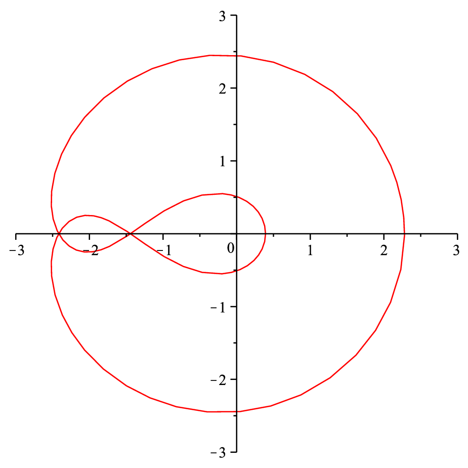
u(z)=\Big(\frac{1}{2}z+1\Big)^{7}.

Refer to caption — Figure 1. On this picture we see the image $u(S)$ . It overlaps around the point $-2$ .

Since we have an overlapping in the image, this map is not primitive. The Theorem A for this example states that if one takes as $\tilde{S}$ the image $u(S)$ , as $\tilde{u}={\mathsf{Id}}$ and as the projection $\pi=u$ then $\tilde{u}:\tilde{S}\to{\mathbb{C}}$ is primitive and $u=\tilde{u}\circ\pi$ .

Remark 1.1.

Let us notice that in the case when $S$ is closed the curve $\tilde{S}$ is also closed and $\pi:S\to\tilde{S}$ is a ramified covering, see Corollary 4.2.

1.2. Positivity of intersections

We denote by $\Delta_{r}$ the disc of radius $r>0$ in ${\mathbb{C}}$ , $\Delta$ stands for $\Delta_{1}$ . Further, let $u_{i}:\Delta\to({\mathbb{C}}^{2},J)$ , $i=1,2$ be two distinct (see Definition 4.1) primitive $J$ -complex discs such that $u_{1}(0)=u_{2}(0)$ . Set $M_{i}\mathrel{\raise 0.3pt\hbox{\rm:}{=}}u_{i}(\Delta)$ . Remark that for Lipschitz-continuous $J$ the notion of multiplicity of zero of a $J$ -holomorphic map is well defined. Namely, due to the Corollary 3.1.3 from [IS1] every non-constant $J$ -holomorphic map $u:(\Delta,0)\to({\mathbb{C}}^{n},J)$ , $J(0)=J_{\mathsf{st}}$ , has the form

u(z)=v_{0}z^{\mu}+O(|z|^{\mu+\alpha}),

(1.2)

where $0\not=v_{0}\in{\mathbb{C}}^{n}$ is called the tangent vector to $u(\Delta)$ at the origin, $\mu\geq 1$ is a natural number, called the multiplicity of $u$ at $0$ , and $0<\alpha<1$ . Our second result is the following

Theorem B. Let $J$ be a Lipschitz-continuous almost complex structure in ${\mathbb{C}}^{2}$ and let $u_{1},u_{2}:\Delta\to{\mathbb{C}}^{2}$ be two distinct $J$ -holomorphic mappings. Then the following holds:

i) For every $0<r<1$ the set $\{\,(z_{1},z_{2})\in\Delta^{2}_{r}:u_{1}(z_{1})=u_{2}(z_{2})\,\}$ is finite.

ii) If $\mu_{1}$ and $\mu_{2}$ are the multiplicities of $u_{1}$ and $u_{2}$ at $z_{1}$ and $z_{2}$ , respectively, with $u_{1}(z_{1})=u_{2}(z_{2})=p$ , then the intersection index $\delta_{p}$ of branches of $M_{1}$ and $M_{2}$ at $z_{1}$ and $z_{2}$ is at least $\mu_{1}\cdot\mu_{2}$ . In particular, $\delta_{p}$ is always strictly positive.

iii) $\delta_{p}=1$ if and only if $M_{1}$ and $M_{2}$ intersect at $p$ transversally.

1.3. Comparison Theorem

Both results of Theorems A and B are obtained using the following statement, which should be considered as the main result of this paper. Let $J$ be a Lipschitz-continuous almost complex structure in the unit ball $B$ in ${\mathbb{C}}^{n}$ and let $u_{1},u_{2}:\Delta\to B$ be two $J$ -holomorphic maps such that $u_{1}(0)=u_{2}(0)=0$ . Assume that both maps have the same order and the same tangent vector at $0$ , i.e., in the representation (1.2) one has

u_{i}(z)=v_{0}z^{\mu}+O(|z|^{\mu+\alpha})\quad\text{ for }\quad i=1,2.

(1.3)

Our goal is to compare these mappings, i.e., to describe in a best possible way their difference.

Comparison Theorem. Let $(X,J)$ be an almost complex manifold with Lipschitz-continuous almost complex structure $J$ and let $u_{i}:\Delta\to X$ be $J$ -holomorphic mappings having the same order and the same tangent vector at $0$ as in (1.3).

(a) There exists a holomorphic function $\psi$ of the form $\psi(z)=z+O(z^{2})$ , an integer $\nu>\mu$ and a ${\mathbb{C}}^{n}$ -valued function $w$ , which belongs to $L^{1,p}_{loc}$ for all $2<p<\infty$ , such that for some $r>0$

u_{2}(z)=u_{1}(\psi(z))+z^{\nu}w(z)\text{ for $z\in\Delta(r)$}.

(1.4)

Moreover, the following alternative holds:

i) either $w(z)$ vanishes identically and then $u_{2}(\Delta(\varepsilon))\subset u_{1}(\Delta)$ for some $\varepsilon>0$ ,

ii) or, the vector $w(0)$ can be chosen orthogonal to $v_{0}$ , in particular, $w(0)\not=0$ and

|{\mathsf{pr}}_{v_{0}}w(z)|\leq C\cdot|z|\,{\mathop{{\mathsf{ln}}}}\frac{1}{|z|}\cdot|w(z)|.

(1.5)

(b) Let $1\not=d\leq\mu$ be a divisor of $\mu$ , and $\eta=e^{2\pi{\mathrm{i}}/d}$ be the primitive root of unity of degree $d$ . Let $u_{1}(\eta z)=u_{1}(\psi(z))+z^{\nu}w(z)$ be the presentation provided by (1.4) for the map $u_{2}(z):=u_{1}(\eta z)$ . Then there exists a holomorphic reparameterization $\varphi$ of the form $\varphi(z)=z+O(z^{2})$ such that

i)

$u_{1}(\varphi(\eta z))\equiv u_{1}(\varphi(z))$ in the case when $w(z)\equiv 0$ ;
ii)

$u_{1}(\varphi(\eta z))=u_{1}(\varphi(z))+w(0)z^{\nu}+O(|z|^{\nu+\alpha})$ otherwise. Moreover, in this case $\nu$ is not a multiple of $d$ .

In (1.5) ${\mathsf{pr}}_{v_{0}}w$ denotes the orthogonal projection of vector $w$ onto the vector $v_{0}$ . Note that $|z|\,{\mathop{{\mathsf{ln}}}}\frac{1}{|z|}=o(|z|^{\alpha})$ for any $0<\alpha<1$ . In fact, from our proof it follows that the vector $w(0)$ can be taken to belong to a prescribed $(n-1)$ -dimensional complex subspace $E_{2}$ of ${\mathbb{C}}^{n}$ transverse to $v_{0}$ , see Remark 3.2. Of course, the choice of $E_{2}$ will affect the reparameterization function $\psi$ and the vector-function $w(z)$ . This theorem is proved in Section 3. Local structure of $J$ -holomorphic maps.

1.4. Optimal regularity of complex curves in Lipschitz structures

Our next result is about the precise regularity of $J$ -complex curves for Lipschitz-continuous $J$ . Recall that a mapping $f$ from a compact set $B\subset{\mathbb{R}}^{n}$ to a normed space is called Log-Lipschitz-continuous if

\left\|{f}\right\|_{{\mathcal{C}}^{LnLip}(B)}\mathrel{\raise 0.3pt\hbox{\rm:}{=}}\left\|{f}\right\|_{L^{\infty}(B)}+{\mathsf{sup}}\,\left\{\frac{|f(x)-f(y)|}{|x-y|\cdot{\mathop{{\mathsf{ln}}}}{\frac{1}{|x-y|}}}:x\not=y\in B,|x-y|\leq\frac{1}{2}\right\}<\infty,

(1.6)

and in this case $\left\|{f}\right\|_{{\mathcal{C}}^{LnLip}(B)}$ is called its Log-Lipschitz norm. Usually one takes $B$ to be the closure of a relatively compact domain $D$ and then one sets $\left\|{f}\right\|_{{\mathcal{C}}^{LnLip}(D)}=\left\|{f}\right\|_{{\mathcal{C}}^{LnLip}(\bar{D})}$ . Without the logarithm in the right hand side (1.6) gives the Lipschitz norm of $f$ , which is denoted by $\left\|{f}\right\|_{{\mathcal{C}}^{Lip}(D)}$ .

Theorem C. Let $u:\Delta\to({\mathbb{R}}^{2n},J)$ be a $J$ -holomorphic map. If $J\in{\mathcal{C}}^{Lip}({\mathbb{R}}^{n})$ then $u\in{\mathcal{C}}^{1,LnLip}$ i.e., the differential of $u$ is Log-Lipschitz-continuous.

We show by a simple example that nothing better can be achieved, in particular $u$ need not belong to ${\mathcal{C}}^{1,Lip}$ .

1.5. Local and global numerical invariants of complex curves

We also prove the following useful formula relating the local and global invariants of a $J$ -complex curve, known as Genus or Adjunction Formula. Let $M=\bigcup_{j=1}^{d}M_{j}$ be a compact $J$ -complex curve in an almost complex surface $(X,J)$ with the distinct irreducible components $\{M_{j}\}$ , where $J$ is Lipschitz-continuous. Denote by $g_{j}$ the genera of parameter curves $S_{j}$ , i.e., each $M_{j}$ is the image $u_{j}(S_{j})$ of a compact Riemann surface $S_{j}$ of genus $g_{j}$ under a primitive $J$ -holomorphic mapping $u_{j}:S_{j}\to X$ . Denote by $[M]^{2}$ the homological self-intersection of $M$ and by $c_{1}(X,J)[M]$ the value of the first Chern class of $(X,J)$ on $M$ . These are the global invariants of $M$ . Denote by $\delta$ the sum of all local intersection indices $\delta_{p}$ of points $p\in M$ . For any singular local branch of $M$ through a point $p$ we define the cusp index $\varkappa_{p}$ as the virtual number of ordinary double points (see Definition 6.1) and denote by $\varkappa$ the sum of the cusp-indices of all cusps of $M$ . These are the local invariants of $M$ . These invariants are related by the following

Theorem D. (Genus Formula) If $J$ is Lipschitz-continuous and $M=\bigcup_{j=1}^{d}M_{j}$ is a compact $J$ -complex curve, where all irreducible components $M_{j}$ of $M$ are distinct, then

\sum_{j=1}^{d}g_{j}=\frac{[M]^{2}-c_{1}(X,J)[M]}{2}+d-\delta-\varkappa.

(1.7)

The novelty here is, of course, in the ability to define the local invariants and to prove that they possess some nice properties (like positivity) under the assumption of Lipschitz continuity of $J$ only. The local intersection indices $\delta_{p}$ are explained by Theorem B. The formula (1.8) below computes the cusp indices $\varkappa_{p}$ .

1.6. Puiseux characteristics of $J$ -complex curves

In the last part of this paper we provide an analog of the Puiseux series for a $J$ -complex curve in a Lipschitz-continuous structure $J$ .

Theorem E. Let $J$ be a Lipschitz-continuous almost complex structure in the unit ball $B\subset{\mathbb{C}}^{n}$ with $J(0)=J_{\mathsf{st}}$ , and let $u:\Delta\to B$ be a primitive $J$ -holomorphic map having the form $u(z)=v_{0}z^{\mu}+O(|z|^{\mu+\alpha})$ , where $\mu\geq 2$ . Then there exist a uniquely defined sequence of natural numbers $p_{0}=\mu<p_{1}<\cdots p_{l}$ , a sequence of vectors $v_{1},\ldots,v_{l}$ each orthogonal to $v_{0}$ , $J$ -holomorphic maps $u_{i}:\Delta_{r}\to B$ , $i=0,\ldots,l$ , and a complex polynomial $\varphi(z)=z+O(z^{2})$ with the following properties:

•

The sequence $d_{i}:={\mathsf{gcd}}(p_{0},\ldots,p_{i})$ is strictly decreasing, $d_{0}>d_{1}>\cdots>d_{l}$ and $d_{l}=1$ ;
•

Each map $u_{i}:\Delta_{r}\to B$ is primitive;
•

$u_{0}(z)=v_{0}z+O(|z|^{1+\alpha})$ , $u_{i}(z)=u_{i-1}(z^{d_{i-1}/d_{i}})+v_{i}\cdot z^{p_{i}/d_{i}}+O(|z|^{p_{i}/d_{i}+\alpha})$ for $i=1,\ldots,l$ ;
•

$u(\varphi(z))-u_{i}(z^{d_{i}})=v_{i+1}z^{p_{i+1}}+O(|z|^{p_{i+1}+\alpha})$ for $i=0,\ldots,l-1$ and $u_{l}(z)=u(\varphi(z))$ ; In particular, if $\eta_{i}:=e^{2\pi{\mathrm{i}}/d_{i}}$ is the primitive root of unity, then

$u(\varphi(\eta_{i}z))-u(\varphi(z))=(\eta_{i}^{p_{i+1}}-1)v_{i+1}z^{p_{i+1}}+O(|z|^{p_{i+1}+\alpha}).$

We call the sequence of the maps $u_{i}(z)$ a Puiseux approximation of the map $u(z)$ , the degrees $p_{0}=\mu<p_{1}<\cdots<p_{l}$ the characteristic exponents, and the numbers $d_{i}={\mathsf{gcd}}(p_{0},\ldots,p_{i})$ the associated divisors. The whole sequence $(p_{0},\ldots,p_{l})$ is called the singularity type of the map $u:\Delta\to B$ at $0$ or of the pseudoholomorphic curve $u(\Delta)=M$ at $0$ . The exponent $p_{0}$ is called the multiplicity or order of $u$ or of the curve $M$ .

In the classical literature ([Co], [BK]) the characteristic exponents are also called essential exponents or even Puiseux characteristics ([Wl]); the difference $p_{0}-p_{1}$ is called the class of the singularity, see e.g. [Co].

Let us illustrate the notions involved in the Theorem E by an example.

Example 2.

Consider a (usual) holomorphic map $u:\Delta\to{\mathbb{C}}^{2}$ given by

u(z)=(z^{6},z^{8}+z^{11}).

Then the $v_{0}=(1,0)$ is the tangent vector at $z=0$ and $\mu=p_{0}=6$ is the multiplicity. Further, its characteristic exponents - where the common divisor drops - are $\mu=p_{0}=6,p_{1}=8,p_{2}=11$ . The corresponding divisors are $d_{0}=p_{0}=6$ , $d_{1}=2$ , $d_{3}=1$ . Further, $v_{1}=e_{2}$ and $v_{2}=e_{2}$ . A Puiseux approximation sequence for $u(z)$ is:
$\bullet\$ $u_{0}(z)=(z,0)$ ,
$\bullet\$ $u_{1}(z)=(z^{3},z^{4})$ ,
$\bullet\$ $u_{2}(z)=u(z)$ .

Finally, we prove that the following classical formula for the index of a cusp of a planar curve

\varkappa_{p}=\frac{1}{2}\sum_{j=1}^{l}(d_{j-1}-d_{j})(p_{j}-1),\quad\text{where}\quad d_{j}\mathrel{\raise 0.3pt\hbox{\rm:}{=}}{\mathsf{gcd}}(p_{0},...,p_{j}),

(1.8)

remains valid for $J$ -complex curves in Lipschitz-continuous $J$ .

1.7. Notes

1. In the classical case, i.e., for algebraic curves the Genus Formula is due to Clebsch and Gordan in the case when the curve in question has only nodal singularities, i.e., transverse intersections, see [CG] and Historical Sketch in [S]. For curves with cusps the Genus Formula is due to Max Noether, see p. 180 in [Fi].

2. The statements of Theorems A and B and the Genus Formula where proved in [MW] for $J\in{\mathcal{C}}^{2}$ . In [Sh] the description of a singularity type of a $J$ -complex curve for $J\in{\mathcal{C}}^{2}$ was given. For $J$ -s of class ${\mathcal{C}}^{1,Lip}$ the positivity of intersections and the part (a) of the Comparison Theorem where proved in [Sk2].

3. Our interest to Lipschitz-continuous structures comes from the following facts. First, a blowing-up of a general almost complex manifold $(X,J)$ , with $J\in{\mathcal{C}}^{\infty}$ , results to an almost complex manifold $(\tilde{X},\tilde{J})$ with only Lipschitz-continuous $\tilde{J}$ . Such a blow-up should be performed in a special coordinate system, adapted to $J$ , see [Du]. It is not difficult to see that the ordinary double points and simple cusps can be resolved by this procedure, as in the classical case, and give a smooth curve. Now the results of the present paper make possible to work with such curves as with usual complex ones.

4. Second, the condition of Lipschitz-continuity cannot be relaxed in any of the statements above. We give an example of two different $J$ -complex curves which coincide by a non-empty open subset for $J$ in all Hölder classes, or $J$ in all $L^{1,p}$ for all $p<\infty$ . In particular, the unique continuation statement of Proposition 3.1 from [FHS] fails to be true. In fact in our example $J$ is “almost” Log-Lipschitz, i.e., is essentially better than $\bigcap_{p<\infty}L^{1,p}$ .

5. At the same time let us point out that even in continuous almost complex structures pseudoholomorphic curves have certain nice properties: every two sufficiently close points can be joined by a $J$ -complex curve, a Fatou-type boundary values theorem is still valid, see [IR2]; Gromov compactness theorem both for compact curves and for curves with boundaries on immersed totally real ( e.g., , Lagrangian) submanifolds hold true for continuous $J$ -s, see [IS3, IS4].

6. To our knowledge the first result about $J$ -complex curves in Lipschitz structures appeared in [NW], where the existence of $J$ -complex curves through a given point in a given direction was proved for $J\in{\mathcal{C}}^{\alpha}$ . Further progress is due to J.-C. Sikorav in [Sk1], see more about that in Remark 3.1 after the proof of Lemma 3.2.

Acknowledgments. This research was partially done during the first authors stay in the Max-Planck-Institute für Mathematik, Bonn. He would like to thank this Institution for the hospitality.

We would like to give our thanks to the Referee of this paper for numerous valuable remarks and suggestions.

2. Zeroes of the Differential of a $J$ -Holomorphic Map

2.1. Inner regularity of pseudoholomorphic maps

Let us first recall few standard facts. For $0<\alpha\leq 1$ consider the Hölder space ${\mathcal{C}}^{k,\alpha}(\Delta,{\mathbb{C}}^{n})$ of mappings $u:\Delta\to{\mathbb{C}}^{n}$ equipped with the norm

\left\|{u}\right\|_{{\mathcal{C}}^{k,\alpha}(\Delta)}:=\left\|{u}\right\|_{{\mathcal{C}}^{k}(\Delta)}+{\mathsf{sup}}\,_{z\not=w,|i|=k}\frac{\left\|{D^{i}u(z)-D^{i}u(w)}\right\|}{|z-w|^{\alpha}}<\infty.

For $k=0$ and $\alpha=1$ the space ${\mathcal{C}}^{0,1}(\Delta,{\mathbb{C}}^{n})$ is the Lipschitz space and is denoted by ${\mathcal{C}}^{Lip}(\Delta,{\mathbb{C}}^{n})$ . The Lipschitz constant of a map $u\in{\mathcal{C}}^{Lip}(\Delta,{\mathbb{C}}^{n})$ is defined as

Lip_{\Delta}(u)\mathrel{\raise 0.3pt\hbox{\rm:}{=}}{\mathsf{sup}}\,_{z\not=w\in\Delta}\frac{\left\|{u(z)-u(w)}\right\|}{|z-w|}.

We also consider Lipschitz continuous (operator valued) functions on relatively compact subsets of ${\mathbb{R}}^{2n}$ with an obvious definitions and notations for them. Another scale of functional spaces, which will be used in this paper, are the Sobolev spaces $L^{k,p}(\Delta,{\mathbb{C}}^{n})$ , $k\in{\mathbb{N}},1\leq p\leq+\infty$ , with the norm

\left\|{u}\right\|_{L^{k,p}(\Delta)}:=\sum_{0\leq|i|\leq k}\left\|{D^{i}u}\right\|_{L^{p}(\Delta)},

where $i=(i_{1},i_{2})$ , with $i_{1},i_{2}\geq 0$ , $|i|=i_{1}+i_{2}$ , and $D^{i}u:=\frac{\partial^{|i|}u}{\partial x^{i_{1}}\partial y^{i_{2}}}$ . Let us also notice the equality $L^{k,\infty}(\Delta,{\mathbb{C}}^{n})={\mathcal{C}}^{k-1,1}(\Delta,{\mathbb{C}}^{n})$ and the continuous Sobolev imbeddings $L^{k,p}(\Delta,{\mathbb{C}}^{n})\hookrightarrow{\mathcal{C}}^{k-1,\alpha}(\Delta,{\mathbb{C}}^{n})$ for $p>2$ and $\alpha=1-\frac{2}{p}$ . We shall frequently use the following notations: $\partial_{x}u:=\frac{\partial u}{\partial x}$ , $\partial_{y}u:=\frac{\partial u}{\partial y}$ and ${\mskip 1.0mu\overline{\mskip-1.0mu{\partial}\mskip-1.0mu}\mskip 1.0mu}u:=\partial_{x}u+i\partial_{y}u$ , i.e., without $\frac{1}{2}$ .

Most considerations in this paper are purely local. Therefore our framework can be described as follows. We consider a Lipschitz-continuous matrix valued function $J$ in the unit ball $B$ of ${\mathbb{C}}^{n}\equiv{\mathbb{R}}^{2n}$ , i.e., $J:B\to$ Mat $(2n\times 2n,{\mathbb{R}})$ such that $J^{2}(x)\equiv-{\mathsf{Id}}$ . Its Lipschitz constant will be denoted by $Lip(J)$ . We are studying $J$ -holomorphic maps $u:\Delta\to B$ . I.e., $u\in{\mathcal{C}}^{0}\cap L^{1,2}(\Delta,B)$ and satisfies

{\mskip 1.0mu\overline{\mskip-1.0mu{\partial}\mskip-1.0mu}\mskip 1.0mu}_{J\circ u}u\mathrel{\raise 0.3pt\hbox{\rm:}{=}}\frac{\partial u}{\partial x}+J(u(z))\frac{\partial u}{\partial y}=0\quad\text{ almost everywhere in }\Delta.

(2.1)

We can consider $J(u(z))=(J\circ u)(z)$ as a matrix valued function on the unit disc, denote it as $J_{u}(z)$ . It satisfies $J_{u}(z)^{2}\equiv-{\mathsf{Id}}$ and therefore it can be viewed as a complex linear structure on the trivial bundle $E:=\Delta\times{\mathbb{R}}^{2n}$ . The mapping $u$ is a section of this bundle. We call the operator ${\mskip 1.0mu\overline{\mskip-1.0mu{\partial}\mskip-1.0mu}\mskip 1.0mu}_{J\circ u}$ the ${\mskip 1.0mu\overline{\mskip-1.0mu{\partial}\mskip-1.0mu}\mskip 1.0mu}$ -operator for the induced structure $J_{u}=J\circ u$ on the bundle $E$ .

Later in this paper we shall use a similar construction as follows. In the trivial bundle $E=\Delta\times{\mathbb{R}}^{2n}(=\Delta\times{\mathbb{C}}^{n})$ over the unit disc consider a complex structure $J(z)$ , i.e., a continuous ${\mathsf{Mat}}(2n\times 2n,{\mathbb{R}})$ -valued function, such that $J(z)^{2}\equiv-{\mathsf{Id}}$ . It defines on $L^{1,2}_{loc}$ - sections of $E$ a ${\mskip 1.0mu\overline{\mskip-1.0mu{\partial}\mskip-1.0mu}\mskip 1.0mu}$ -type operator

{\mskip 1.0mu\overline{\mskip-1.0mu{\partial}\mskip-1.0mu}\mskip 1.0mu}_{J}u\mathrel{\raise 0.3pt\hbox{\rm:}{=}}\frac{\partial u}{\partial x}+J(z)\frac{\partial u}{\partial y}.

(2.2)

Therefore we can interpret (2.1) saying that a $J$ -holomorphic map $u$ is a section of $E$ , which satisfies (2.2) with $J(z)=J_{u}(z)$ .

In the Proposition 2.1 below we shall see that $u$ satisfying (2.1) is, in fact, of class ${\mathcal{C}}^{1,\alpha}$ for all $0<\alpha<1$ .

Proposition 2.1.

Let $J$ be an ${\mathsf{End}}({\mathbb{R}}^{2n})$ -valued function on $\Delta$ of class ${\mathcal{C}}^{k-1,Lip}$ , $k\geq 1$ , and let $R$ be an ${\mathsf{End}}({\mathbb{R}}^{2n})$ -valued function on $\Delta$ of class $L^{k,p}$ , $1<p<\infty$ . Suppose that $J^{2}\equiv-{\mathsf{Id}}$ and that ${\mskip 1.0mu\overline{\mskip-1.0mu{\partial}\mskip-1.0mu}\mskip 1.0mu}_{J}u+Ru\in L^{k,p}(\Delta)$ for some $u\in L^{1,2}(\Delta,{\mathbb{R}}^{2n})$ . Then $u\in L^{k+1,p}_{{\mathsf{loc}}}(\Delta,{\mathbb{R}}^{2n})$ and for $0<r<1$

\hbox{ }\left\|{u}\right\|_{L^{k+1,p}(\Delta(r))}\leq C_{k,p}\bigl(\left\|{{\mskip 1.0mu\overline{\mskip-1.0mu{\partial}\mskip-1.0mu}\mskip 1.0mu}_{J}u+Ru}\right\|_{L^{k,p}(\Delta)}+\left\|{u}\right\|_{L^{p}(\Delta)}\bigr),

(2.3)

where $C_{k,p}=C(\left\|{J}\right\|_{{\mathcal{C}}^{k-1,Lip}},\left\|{R}\right\|_{L^{k,p}},k,p,r)<\infty$ . Moreover, there exists an $\varepsilon=\varepsilon(k,p)>0$ such that if

\left\|{J-J_{\mathsf{st}}}\right\|_{{\mathcal{C}}^{k-1,Lip}(\Delta)}+\left\|{R}\right\|_{L^{k,p}(\Delta)}<\varepsilon

then the constant $C_{k,p}$ above can be chosen to be independent of $||J||$ and $||R||$ .

For the proof see [M], Theorem 6.2.5. The condition $J^{2}\equiv-{\mathsf{Id}}$ is needed in this statement to insure the ellipticity of the operator ${\mskip 1.0mu\overline{\mskip-1.0mu{\partial}\mskip-1.0mu}\mskip 1.0mu}_{J}$ . We shall use in this paper the case $k=1$ only. Remark that our initial assumption on $u$ is $u\in L^{1,2}(\Delta)$ which implies that $u\in L^{p}(\Delta)$ for all $p<\infty$ . This proposition implies, in particular, that a $J$ -holomorphic map $u:\Delta\to{\mathbb{R}}^{2n}$ is of class $L^{2,p}_{{\mathsf{loc}}}(\Delta)$ for all $p<\infty$ provided $J$ is Lipschitz. In particular $u\in{\mathcal{C}}^{1,\alpha}_{loc}(\Delta)$ for all $0<\alpha<1$ .

2.2. Estimation of the differential at cusp-points

Throughout this subsection we fix some $2<p<\infty$ and make the following assumption:

$(*)$

$J$ is an almost complex structure in $B$ with $J(0)=J_{\mathsf{st}}$ such that $\left\|{J-J_{\mathsf{st}}}\right\|_{{\mathcal{C}}^{Lip}(B)}$ is small enough. $u:\Delta\to B$ is a $J$ -holomorphic map such that $u(0)=0$ and such that $\left\|{du}\right\|_{L^{1,p}(\Delta)}$ is small enough.

Let us notice that this assumption is by no means restrictive. Indeed, we can always replace $J(w)$ by $J_{\tau}(w):=J(\tau w)$ and $u(z)$ by $u_{t,\tau}(z):=\tau^{-1}u(tz)$ with some appropriately chosen $\tau$ and $t$ .

By the Corollary 3.1.3 from [IS1] (see also Proposition 3 in [Sk2] and the corresponding Corollary 1.4.3 in [IS2]) we can assign multiplicity of zero to a $J$ -holomorphic map $u:\Delta\to(B,J)$ provided that $J$ is at least Lipschitz. In particular, zeroes of $u$ are isolated, as for the classical holomorphic functions. Moreover, we can represent such $u$ (in the neighborhood of its zero point, say $z_{0}=0$ , provided $J(0)=J_{\mathsf{st}}$ ) as

u(z)=z^{\mu}P(z)+z^{2\mu-1}v(z),

(2.4)

where $\mu\geq 1$ is an integer (a multiplicity of zero), $P(z)$ is some (holomorphic) polynomial of degree at most $\mu-1$ , $P(0)\not=0$ and $v\in L^{1,p}_{loc}(\Delta,{\mathbb{C}}^{n})$ for all $2<p<\infty$ , and therefore $v\in{\mathcal{C}}^{\alpha}(\Delta,{\mathbb{C}}^{n})$ for all $0<\alpha<1$ . In addition, $v(0)=0$ . Now we want to derive from (2.4) some properties of the differential $du$ .

Let us start with the following preliminary estimate.

Lemma 2.1.

For any integer $\mu\geq 1$ there exists a constant $C=C(\mu,p)<\infty$ with the following property: for every $J$ -holomorphic map $u:\Delta\to(B,J)$ , satisfying the assumption (*) and having the form (2.4) one has

\left\|{v}\right\|_{L^{1,p}(\Delta)}\leq C\cdot\left\|{u}\right\|_{L^{1,p}(\Delta)}.

(2.5)

Proof. We use the fact that every $J$ -holomorphic map $u:\Delta\to B$ with Lipschitz-continuous $J$ satisfies the pointwise estimate

|{\mskip 1.0mu\overline{\mskip-1.0mu{\partial}\mskip-1.0mu}\mskip 1.0mu}_{\mathsf{st}}u(z)|\leq Lip(J)\cdot|du(z)|\cdot|u(z)|,

(2.6)

see inequality (1.4.4) in [IS2]. Following [Sk1] define

H(z):=\begin{cases}\textstyle\ -\frac{{\mskip 1.0mu\overline{\mskip-1.0mu{\partial}\mskip-1.0mu}\mskip 1.0mu}_{\mathsf{st}}u(z)\otimes\bar{u}(z)}{|u(z)|^{2}}&\text{ if }\quad u(z)\not=0,\\ \ 0&\text{ if }\quad u(z)=0.\end{cases}

(2.7)

Then $H(z)$ is a measurable function with values in ${\mathsf{Mat}}_{{\mathbb{C}}}(n\times n)$ , which satisfies the pointwise estimate

|H(z)|\leq Lip(J)\cdot|du(z)|.

(2.8)

In particular, $\left\|{H(z)}\right\|_{L^{p}(\Delta)}$ is bounded by some sufficiently small constant by the assumption $(*)$ . The function $u(z)$ in its turn satisfies

{\mskip 1.0mu\overline{\mskip-1.0mu{\partial}\mskip-1.0mu}\mskip 1.0mu}_{\mathsf{st}}u(z)+H(z)\cdot u(z)=0.

(2.9)

Under these conditions Lemma 1.2.3 from [IS2] insures the existence of a matrix-valued function $F(z)\in L^{1,p}(\Delta)$ which satisfies the equation

{\mskip 1.0mu\overline{\mskip-1.0mu{\partial}\mskip-1.0mu}\mskip 1.0mu}_{\mathsf{st}}F=-F\cdot H.

(2.10)

with the estimate

\left\|{F(z)-{\mathsf{Id}}}\right\|_{L^{1,p}(\Delta)}\leq C\cdot\left\|{H(z)}\right\|_{L^{p}(\Delta)}

(2.11)

The equations (2.9) and (2.10) imply that the function $F(z){\cdot}u(z)$ is holomorphic. Define $u^{(\mu)}(z):=z^{-\mu}u(z)$ . It satisfies ${\mskip 1.0mu\overline{\mskip-1.0mu{\partial}\mskip-1.0mu}\mskip 1.0mu}_{\mathsf{st}}(Fu^{(\mu)}(z))=0$ and relation (2.4) implies that the function $F(z){\cdot}u^{(\mu)}(z)=z^{-\mu}F(z){\cdot}u(z)$ has no pole at zero and therefore is holomorphic.

Since $\left\|{F(z)-{\mathsf{Id}}}\right\|_{L^{1,p}(\Delta)}$ is small we have that for any domain $A\subset\Delta$ the following inequality

c_{\mu}\left\|{u^{(\mu)}}\right\|_{L^{1,p}(\Delta)}\leq\left\|{F(z)\cdot u^{(\mu)}(z)}\right\|_{L^{1,p}(\Delta)}\leq C_{\mu}\left\|{u^{(\mu)}}\right\|_{L^{1,p}(\Delta)}.

Observe that $F(z)\cdot u^{(\mu)}(z)$ satisfies

\left\|{F\cdot u^{(\mu)}}\right\|_{L^{1,p}(\Delta)}\leq C_{1}\left\|{F\cdot u^{(\mu)}}\right\|_{L^{1,p}(\Delta\backslash\Delta({\frac{1}{2}}))}.

(2.12)

This easily follows from the Cauchy integral formula for the Taylor coefficients of holomorphic function. Consequently we get

\left\|{F\cdot u^{(\mu)}}\right\|_{L^{1,p}(\Delta)}\leq C\cdot\left\|{u^{(\mu)}}\right\|_{L^{1,p}(\Delta\backslash\Delta({\frac{1}{2}}))}.

(2.13)

This gives us the estimate

\left\|{u^{(\mu)}}\right\|_{L^{1,p}(\Delta)}\leq C_{\mu}\cdot\left\|{u}\right\|_{L^{1,p}(\Delta)},

(2.14)

because on the annulus $\Delta\backslash\Delta({\frac{1}{2}})$ functions $u$ and $u^{(\mu)}$ are comparable. The latter estimate implies that $d(u(z))=d(z^{\mu}u^{(\mu)}(z))$ fulfills a.-e. the estimate

|du(z)|\leq h(z)\cdot|z^{\mu-1}|

(2.15)

for some non-negative $L^{p}$ -function $h$ satisfying

\left\|{h}\right\|_{L^{p}(\Delta)}\leq C\cdot\left\|{u}\right\|_{L^{1,p}(\Delta)}.

(2.16)

Substituting the relation (2.15) in (2.6) we obtain a.-e. the pointwise estimate

|{\mskip 1.0mu\overline{\mskip-1.0mu{\partial}\mskip-1.0mu}\mskip 1.0mu}_{\mathsf{st}}u(z)|\leq C\cdot|z^{\mu-1}|\cdot h(z)\cdot|u(z)|

with the same function $h\in L^{p}(\Delta)$ as above. Multiplying it by $z^{-\mu}$ we obtain

|{\mskip 1.0mu\overline{\mskip-1.0mu{\partial}\mskip-1.0mu}\mskip 1.0mu}_{\mathsf{st}}u^{(\mu)}(z)|\leq C\cdot|z^{\mu-1}|\cdot h(z)\cdot|u^{(\mu)}(z)|.

(2.17)

For $j=1,\ldots,\mu-1$ define functions $u^{(\mu+j)}(z)$ recursively by the relation

u^{(\mu+j)}(z):=(u^{(\mu+j-1)}(z)-u^{(\mu+j-1)}(0))/z.

Then the coefficients of the polynomial $P(z)$ from (2.4) are given by $a_{j}=u^{(\mu+j)}(0)$ for $j=0,\ldots,\mu-1$ and $v(z)=u^{(2\mu-1)}(z)-u^{(2\mu-1)}(0)$ .

We claim that for every $j=0,\ldots,\mu-1$ we have the estimation

\left\|{u^{(\mu+j)}}\right\|_{L^{1,p}(\Delta)}\leq C\cdot\left\|{u}\right\|_{L^{1,p}(\Delta)},

(2.18)

and therefore $|a_{j}|\leq C\cdot\left\|{u}\right\|_{L^{1,p}(\Delta)}$ . The proof is done by induction using (2.14) as the base for $j=0$ . Thus we assume that for some fixed $j\in\{1,\ldots,\mu-1\}$ we have the estimation of the form $\left\|{u^{(\mu+j-1)}}\right\|_{L^{1,p}(\Delta)}\leq C\cdot\left\|{u}\right\|_{L^{1,p}(\Delta)}$ , and in particular $|a_{j-1}|=|u^{(\mu+j-1)}(0)|\leq C\cdot\left\|{u}\right\|_{L^{1,p}(\Delta)}$ . From the definition of $u^{(\mu+j)}(z)$ we obtain a.-e. the pointwise differential inequality

\begin{split}|{\mskip 1.0mu\overline{\mskip-1.0mu{\partial}\mskip-1.0mu}\mskip 1.0mu}_{\mathsf{st}}u^{(\mu+j)}(z)|\;&=|z^{-1}{\mskip 1.0mu\overline{\mskip-1.0mu{\partial}\mskip-1.0mu}\mskip 1.0mu}_{\mathsf{st}}u^{(\mu+j-1)}(z)|=|z^{-2}{\mskip 1.0mu\overline{\mskip-1.0mu{\partial}\mskip-1.0mu}\mskip 1.0mu}_{\mathsf{st}}u^{(\mu+j-2)}(z)|=\ldots=\\ &=|z^{-j}{\mskip 1.0mu\overline{\mskip-1.0mu{\partial}\mskip-1.0mu}\mskip 1.0mu}_{\mathsf{st}}u^{(\mu)}(z)|\leq C\cdot h(z)\cdot|z^{\mu-1-j}|\cdot|u^{(\mu)}(z)|.\end{split}

This gives the estimate

\left\|{{\mskip 1.0mu\overline{\mskip-1.0mu{\partial}\mskip-1.0mu}\mskip 1.0mu}_{\mathsf{st}}u^{(\mu+j)}(z)}\right\|_{L^{p}(\Delta)}\leq C\left\|{h}\right\|_{L^{p}(\Delta)}\left\|{u^{(\mu)}}\right\|_{L^{\infty}(\Delta)}\leq C_{1}\left\|{u}\right\|_{L^{1,p}(\Delta)}

(2.19)

by (2.14) and (2.16). Further

\left\|{u^{(\mu+j)}}\right\|_{L^{1,p}(\Delta\backslash\Delta({\frac{1}{2}}))}\leq C\cdot\big(a_{j-1}+\left\|{u^{(\mu+j-1)}}\right\|_{L^{1,p}(\Delta\backslash\Delta({\frac{1}{2}}))}\big)\leq C_{1}\cdot\left\|{u}\right\|_{L^{1,p}(\Delta)}

by inductive assumption. Now the standard inner estimates for ${\mskip 1.0mu\overline{\mskip-1.0mu{\partial}\mskip-1.0mu}\mskip 1.0mu}_{\mathsf{st}}$ provide the desired estimates

\left\|{u^{(\mu+j)}}\right\|_{L^{1,p}(\Delta)}\leq C\cdot\left\|{u}\right\|_{L^{1,p}(\Delta)}\qquad\text{and}\qquad|a_{j}|\leq C\cdot\left\|{u}\right\|_{L^{1,p}(\Delta)}.

The case $j=\mu-1$ yields the estimate (2.5) on $v(z)=u^{(2\mu-1)}(z)-a_{\mu-1}$ .

$\square$

The following lemma will be used in this paper with various operators $A$ .

Lemma 2.2.

Let $A$ be a Lipschitz continuous ${\mathsf{End}}({\mathbb{R}}^{2n})$ -valued function on $B$ with $A(0)=0$ and let $u$ be a $J$ -holomorphic map with Lipschitz $J$ as in (2.4). Then for all integers $\nu$ and $\lambda$ satisfying $\nu\leq\mu+\lambda-1$ the function $z^{-\nu}\cdot A(u(z))\cdot z^{\lambda}$ is Lipschitz-continuous in $\Delta$ with the estimate

Lip_{\Delta}(z^{-\nu}\cdot A(u(z))\cdot z^{\lambda})\leq C(p)\cdot Lip(A)\cdot\left\|{u}\right\|_{L^{1,p}(\Delta)}.

(2.20)

Proof. Remark that we have the following estimate

\left\|{z^{-\mu}u(z)}\right\|_{L^{\infty}(\Delta(\frac{2}{3}))}\leq C\cdot\left\|{u}\right\|_{L^{1,p}(\Delta)}.

(2.21)

This is clear because in (2.14) a $L^{1,p}$ and therefore a ${\mathcal{C}}^{\alpha}$ - norm of $u^{(\mu)}=z^{-\mu}u$ was estimated.

We continue the proof of the lemma starting from the remark that since $u$ is $J$ -holomorphic with Lipschitz $J$ , it is of class ${\mathcal{C}}^{1,\alpha}$ and therefore itself Lipschitz.

Now we turn to the estimation of the quantity $\frac{\left\|{z^{-\nu}_{1}A(u(z_{1}))z^{\lambda}_{1}-z^{-\nu}_{2}A(u(z_{2}))z^{\lambda}_{2}}\right\|}{|z_{1}-z_{2}|}$ for $z_{1}\not=z_{2}\in\Delta$ . In order to do this we consider two cases.

Case 1. $\frac{1}{3}|z_{1}|\leq|z_{1}-z_{2}|$ . In that case $|z_{1}|\leq 3|z_{1}-z_{2}|$ and $|z_{2}|\leq 4|z_{1}-z_{2}|$ . Therefore

\frac{\left\|{z^{-\nu}_{1}A(u(z_{1}))z^{\lambda}_{1}-z^{-\nu}_{2}A(u(z_{2}))z^{\lambda}_{2}}\right\|}{|z_{1}-z_{2}|}=

=\frac{\left\|{z^{-\nu}_{1}A(u(z_{1}))z^{\lambda}_{1}-z^{-\nu}_{1}A(u(0))z^{\lambda}_{1}+z^{-\nu}_{2}A(u(0))z^{\lambda}_{2}-z^{-\nu}_{2}A(u(z_{2}))z^{\lambda}_{2}}\right\|}{|z_{1}-z_{2}|}\leq

\leq C\cdot Lip(A)\left\|{z^{-\mu}u(z)}\right\|_{L^{\infty}}\frac{|z_{1}|^{\mu+\lambda-\nu}+|z_{2}|^{\mu+\lambda-\nu}}{|z_{1}-z_{2}|}\leq

\leq C\cdot Lip(A)\left\|{z^{-\mu}u(z)}\right\|_{L^{\infty}}\frac{|z_{1}|+|z_{2}|}{|z_{1}-z_{2}|}\leq C\cdot Lip(A)\left\|{u(z)}\right\|_{L^{1,p}(\Delta)},

because $\mu+\lambda-\nu\geq 1$ . In the second line we silently used the fact that $A(u(0))=0$ .

Case 2. $|z_{1}-z_{2}|\leq\frac{1}{3}|z_{1}|$ . In that case $\frac{2}{3}|z_{1}|\leq|z_{2}|\leq\frac{4}{3}|z_{1}|$ . Therefore

\frac{\left\|{z^{-\nu}_{1}A(u(z_{1}))z^{\lambda}_{1}-z^{-\nu}_{2}A(u(z_{2}))z^{\lambda}_{2}}\right\|}{|z_{1}-z_{2}|}\leq\frac{\left\|{z^{-\nu}_{1}A(u(z_{1}))z^{\lambda}_{1}-z^{-\nu}_{1}A(u(z_{1}))z^{\lambda}_{2}}\right\|}{|z_{1}-z_{2}|}+

+\frac{\left\|{z^{-\nu}_{1}A(u(z_{1}))z^{\lambda}_{2}-z^{-\nu}_{2}A(u(z_{1}))z^{\lambda}_{2}}\right\|}{|z_{1}-z_{2}|}+\frac{\left\|{z^{-\nu}_{2}A(u(z_{1}))z^{\lambda}_{2}-z^{-\nu}_{2}A(u(z_{2}))z^{\lambda}_{2}}\right\|}{|z_{1}-z_{2}|}=

=\frac{\left\|{z^{-\nu}_{1}A(u(z_{1}))[z^{\lambda}_{1}-z^{\lambda}_{2}]}\right\|}{|z_{1}-z_{2}|}+\frac{\left\|{[z^{-\nu}_{1}-z^{-\nu}_{2}]A(u(z_{1}))z^{\lambda}_{2}}\right\|}{|z_{1}-z_{2}|}+\frac{\left\|{z^{-\nu}_{2}[A(u(z_{1}))-A(u(z_{2}))]z^{\lambda}_{2}}\right\|}{|z_{1}-z_{2}|}=

=I_{1}+I_{2}+I_{3}.

Let us estimate these terms separately. First:

I_{1}\leq|z_{1}|^{-\nu}\left\|{A(u(z_{1}))}\right\|\sum_{j=0}^{\lambda-1}|z_{1}^{j}z_{2}^{\lambda-j-1}|

\leq C\cdot Lip(A)\left\|{z^{-\mu}u(z)}\right\|_{L^{\infty}(\Delta(\frac{2}{3}))}|z_{1}|^{-\nu+\mu}|z_{1}|^{\lambda-1}\leq C\cdot Lip(A)\left\|{u}\right\|_{L^{1,p}(\Delta)}.

Second:

I_{2}\leq C\cdot Lip(A)\left\|{z^{-\mu}u(z)}\right\|_{L^{\infty}(\Delta(\frac{2}{3}))}\;|z_{1}|^{\mu}\;|z_{2}|^{\lambda}\left|\frac{z_{2}-z_{1}}{z_{1}z_{2}}\right|\left(\sum_{j=0}^{\nu-1}\left|z_{1}^{-j}z_{2}^{-(\nu-j-1)}\right|\right)\frac{1}{|z_{1}-z_{2}|}

\leq C\cdot Lip(A)\left\|{u}\right\|_{L^{1,p}(\Delta)}|z_{1}|^{\lambda+\mu-\nu-1}\leq C\cdot Lip(A)\left\|{u}\right\|_{L^{1,p}(\Delta)}.

And, finally, third:

I_{3}\leq C\cdot Lip(A)\left\|{z^{-\mu}u(z)}\right\|_{L^{\infty}(\Delta(\frac{2}{3}))}|z_{2}|^{-\nu}|z_{1}^{\mu}-z_{2}^{\mu}|\;|z_{2}|^{\lambda}\;\frac{1}{|z_{1}-z_{2}|}\leq C\cdot Lip(A)\left\|{u}\right\|_{L^{1,p}(\Delta)}.

$\square$

We need to produce some extra regularity of the rest term $zv(z)$ in the representation (2.4). In fact we shall prove that $z\cdot v\in L^{2,p}_{{\mathsf{loc}}}(\Delta)$ for $v$ from (2.4) together with the estimate of its decay at zero.

Lemma 2.3.

Let $J$ be a Lipschitz-continuous almost complex structure in the unit ball $B\subset{\mathbb{C}}^{n}$ with $J(0)=J_{\mathsf{st}}$ and $u:\Delta\to B$ be a $J$ -holomorphic map written in the form (2.4). Then $zv\in L^{2,p}_{{{\mathsf{loc}}}}$ for all $2<p<\infty$ . Moreover, for every $|z|\leq\frac{1}{2}$ one has

|d(zv(z))|\leq C(p)\cdot|z|^{1-\frac{2}{p}}\cdot\|u\|_{L^{1,p}(\Delta)}

(2.22)

for with the constant $C(p)$ independent of $z$ , $u$ and $J$ satisfying the assumption (*).

Proof. Remark that with $\nu=2\mu-2$ in Lemma 2.2 above we have

z^{\nu}\cdot(zv(z))=u(z)-z^{\mu}\cdot P(z).

(2.23)

So if we apply ${\mskip 1.0mu\overline{\mskip-1.0mu{\partial}\mskip-1.0mu}\mskip 1.0mu}_{J\circ u}$ to the right hand side of (2.23) we obtain ${\mskip 1.0mu\overline{\mskip-1.0mu{\partial}\mskip-1.0mu}\mskip 1.0mu}_{J\circ u}(z^{\mu}P)$ which is Lipschitz continuous, in particular, it belongs to $L^{1,p}_{loc}$ for all $1<p<\infty$ . Elliptic regularity of Proposition 2.1 gives then the $L^{2,p}$ -regularity of the left hand side $z^{\nu}\cdot(zv(z))$ . If $\mu=1$ (and therefore $\nu=0$ ), then $zv(z)=u(z)\in L^{2,p}_{{\mathsf{loc}}}(\Delta)$ , and the needed $L^{2,p}$ -regularity is already proved. Therefore till the Step 4 we shall suppose that $\mu\geq 2$ .

Let us explain the idea of the proof of this lemma. First we observe that

z^{-\nu}\left[\partial_{x}+J(u(z))\partial_{y}\right]z^{\nu}(zv)=(\partial_{x}+z^{-\nu}J(u)z^{\nu}\partial_{y})(zv)+z^{-\nu}(1+J(u)J_{\mathsf{st}})\nu z^{\nu-1}(zv).

(2.24)

We see (2.24) as the equation of the form

f(z)=\left({\mskip 1.0mu\overline{\mskip-1.0mu{\partial}\mskip-1.0mu}\mskip 1.0mu}_{J^{(\nu)}}+R^{(\nu)}\right)(zv(z)).

(2.25)

After establishing the necessary regularity of $J^{\nu)}$ , $R^{(\nu)}$ and $f$ we shall apply the Proposition 2.1 and obtain the desired regularity of the solution $zv$ .

Let us start with the right hand side of (2.24).

Step 1. $J^{(\nu)}\mathrel{\raise 0.3pt\hbox{\rm:}{=}}z^{-\nu}\cdot J(u)\cdot z^{\nu}$ is a Lipschitz continuous complex structure on $E$ and $Lip(J^{(\nu)})\leq C\cdot Lip(J)\cdot\left\|{u}\right\|_{L^{1,p}(\Delta)}$ .

The proof is straightforward via Lemma 2.2: just write $J^{(\nu)}=z^{-\nu}[J(u)-J_{\mathsf{st}}]z^{\nu}+J_{\mathsf{st}}$ and apply Lemma 2.2 to $A=J-J_{\mathsf{st}}$ .

Step 2. The endomorphism $R^{(\nu)}\mathrel{\raise 0.3pt\hbox{\rm:}{=}}z^{-\nu}\cdot(1+J(u)J_{\mathsf{st}})\nu z^{\nu-1}$ of the bundle $E$ is Lipschitz continuous, $R^{(\nu)}(0)=0$ and $Lip(R^{(\nu)})\leq C\cdot Lip(J)\cdot\left\|{u}\right\|_{L^{1,p}(\Delta)}$ .

This is again true by Lemma 2.2 and because $\mu\geq 2$ . Note now that the right hand side of (2.24) is of the form ${\mskip 1.0mu\overline{\mskip-1.0mu{\partial}\mskip-1.0mu}\mskip 1.0mu}_{J^{(\nu)}}(zv)+R^{(\nu)}(zv)$ and that coefficients of this operator are Lipschitz continuous. Therefore we can apply (2.3) and obtain

\left\|{zv}\right\|_{L^{2,p}(\Delta(1/2))}\leq C\big(\left\|{{\mskip 1.0mu\overline{\mskip-1.0mu{\partial}\mskip-1.0mu}\mskip 1.0mu}_{J^{(\nu)}}(zv)+R^{(\nu)}(zv)}\right\|_{L^{1,p}(\Delta)}+\left\|{zv}\right\|_{L^{p}(\Delta)}\big).

(2.26)

To achieve (2.22) for $r=\frac{1}{2}$ we need to estimate both terms in the right hand side (2.26) by $\left\|{u}\right\|_{L^{1,p}(\Delta)}$ . For the term $zv(z)$ it was already done in (2.5). In order to estimate the first term we shall compute the left hand side of (2.24) in another way. Namely, using (2.4) we write

z^{-\nu}\left[\partial_{x}+J(u(z))\partial_{y}\right]z^{\nu}(zv)=z^{-\nu}\left[\partial_{x}+J(u(z))\partial_{y}\right](u(z)-z^{\mu}\cdot P(z))=

=z^{-\nu}\left[\partial_{x}+J(u(z))\partial_{y}\right](-z^{\mu}\cdot P(z))=z^{-\nu}\left[\partial_{x}+J(u(z))\partial_{y}\right](\sum_{j=0}^{\mu-1}a_{j}z^{\mu+j})=

=z^{-\nu}(1+J(u)J_{\mathsf{st}})(\sum_{j=0}^{\mu-1}(\mu+j)a_{j}z^{\mu+j-1})=:f(z).

(2.27)

Step 3. The right hand side $f(z)$ of (2.27) satisfies $f(0)=0$ and is Lipschitz continuous with the estimate

\left\|{f}\right\|_{{\mathcal{C}}^{Lip}(\Delta)}\leq C\left\|{J}\right\|_{{\mathcal{C}}^{Lip}(\Delta)}\left\|{u}\right\|_{L^{1,p}(\Delta)}.

(2.28)

The worst term is $z^{-\nu}(1+J(u)J_{\mathsf{st}})(\mu a_{0}z^{\mu-1})$ , but it is still under control of the Lemma 2.2. We conclude now by (2.26) and (2.28) the estimate

\left\|{d(zv)}\right\|_{L^{1,p}(\Delta(1/2))}\leq C\cdot\left\|{u}\right\|_{L^{1,p}(\Delta)}.

(2.29)

Step 4. The behavior of $z\,v(z)$ under a dilatation.

For $\tau\in[0,1]$ and we define $\pi_{\tau}:\Delta\to\Delta$ by $\pi_{\tau}(z):=\tau\cdot z$ . Then for any function $w(z)$ in the disc $\pi_{\tau}^{*}w(z)=w(\tau z)$ is the dilatation of $w(z)$ . An easy calculation shows the following dilatation behavior of the $L^{p}$ -norms of the derivatives:

\left\|{D^{i}(\pi_{\tau}^{*}w)}\right\|_{L^{p}(\Delta)}=\tau^{|i|-\frac{2}{p}}\left\|{D^{i}w}\right\|_{L^{p}(\Delta(\tau))}.

Estimating $L^{p}$ -norm we use the fact that $v(0)=0$ and that $\left\|{v}\right\|_{{\mathcal{C}}^{\alpha}(\Delta)}\leq C\cdot\left\|{u(z)}\right\|_{L^{1,p}(\Delta)}$ , see Lemma 2.1. Hence $|v(z)|\leq C\cdot|z|^{\alpha}\cdot\left\|{u(z)}\right\|_{L^{1,p}(\Delta)}$ and thus (using $\alpha=1-\frac{2}{p}$ )

\left\|{zv(z)}\right\|_{L^{p}(\Delta(r))}\leq\left\|{zv(z)}\right\|_{L^{\infty}(\Delta(r))}(\pi r^{2})^{\frac{1}{p}}\leq C\cdot r^{2}\cdot\left\|{u(z)}\right\|_{L^{1,p}(\Delta)}.

Consequently

\left\|{\pi^{*}_{r}(zv(z))}\right\|_{L^{p}(\Delta)}\leq C\cdot r^{2-\frac{2}{p}}\cdot\left\|{u(z)}\right\|_{L^{1,p}(\Delta)}.

Now recall that $zv(z)$ satisfies the differential equation

\left({\mskip 1.0mu\overline{\mskip-1.0mu{\partial}\mskip-1.0mu}\mskip 1.0mu}_{J^{(\nu)}}+R^{(\nu)}\right)(zv(z))=f(z)

with $f(z)$ given by the formula (2.27). By Step 3, $f(z)$ is Lipschitz continuous with the estimate (2.28) and $f(0)=0$ . This implies that

\left\|{\pi_{r}^{*}f(z)}\right\|_{{\mathcal{C}}^{Lip}(\Delta)}\leq C\cdot r\cdot\left\|{J}\right\|_{{\mathcal{C}}^{Lip}(\Delta)}\left\|{u(z)}\right\|_{L^{1,p}(\Delta)}.

The same argument yields also

\left\|{\pi_{r}^{*}(J^{(\nu)}-J_{\mathsf{st}})}\right\|_{{\mathcal{C}}^{Lip}(\Delta)}\leq r\cdot\left\|{J^{(\nu)}-J_{\mathsf{st}}}\right\|_{{\mathcal{C}}^{Lip}(\Delta)}.

Finally, we observe that

\pi^{*}_{r}\big({\mskip 1.0mu\overline{\mskip-1.0mu{\partial}\mskip-1.0mu}\mskip 1.0mu}_{J^{(\nu)}}(zv(z))\big)=r^{-1}\cdot{\mskip 1.0mu\overline{\mskip-1.0mu{\partial}\mskip-1.0mu}\mskip 1.0mu}_{\pi^{*}_{r}J^{(\nu)}}(\pi^{*}_{r}(zv(z))).

Summing up, we see that the rescaled function $w_{r}(z):=\pi^{*}_{r}(zv(z))$ satisfies a ${\mskip 1.0mu\overline{\mskip-1.0mu{\partial}\mskip-1.0mu}\mskip 1.0mu}$ -type equation

\big({\mskip 1.0mu\overline{\mskip-1.0mu{\partial}\mskip-1.0mu}\mskip 1.0mu}_{\pi^{*}_{r}J^{(\nu)}}+r\cdot\pi_{r}^{*}R^{(\nu)}\big)w_{r}(z)=r\cdot\pi_{r}^{*}f(z)

in which the norms $\left\|{r\cdot\pi_{r}^{*}f(z)}\right\|_{{\mathcal{C}}^{Lip}(\Delta)}$ are bounded by $C\cdot r^{2}\cdot\left\|{u}\right\|_{L^{1,p}(\Delta)}$ uniformly in $r$ and the coefficients $\pi^{*}_{r}J^{(\nu)}$ and $r\cdot\pi^{*}_{r}R^{(\nu)}$ are ${\mathcal{C}}^{Lip}$ -close to those of ${\mskip 1.0mu\overline{\mskip-1.0mu{\partial}\mskip-1.0mu}\mskip 1.0mu}_{\mathsf{st}}$ for $r$ close enough to $0$ .

From Proposition 2.1 we obtain the uniform estimate

\left\|{\pi^{*}_{r}(zv(z))}\right\|_{L^{2,p}(\Delta)}\leq C\cdot r^{2-\frac{2}{p}}\cdot\left\|{u}\right\|_{L^{1,p}(\Delta)},

which implies

\left\|{d(\pi^{*}_{r}(zv(z)))}\right\|_{L^{\infty}(\Delta)}\leq C\cdot r^{2-\frac{2}{p}}\cdot\left\|{u}\right\|_{L^{1,p}(\Delta)}.

After rescaling we obtain

\left\|{d(zv(z))}\right\|_{L^{\infty}(\Delta(r))}\leq C\cdot r^{\alpha}\cdot\left\|{u}\right\|_{L^{1,p}(\Delta)},

with $\alpha=1-\frac{1}{p}$ . $\square$

The estimate (2.22) gives immediately the following

Corollary 2.1.

For a Lipschitz-continuous $J$ and $J$ -holomorphic $u$ in the form (2.4) one has

du(z)=d(z^{\mu}P(z))+O(|z|^{2\mu-2+\alpha}).

(2.30)

for any $0<\alpha<1$ . In particular, for a non-constant $u$ zeroes of $du$ are isolated.

2.3. An example

Let us illustrate the statements of this Section by an example.

Example 3.

Equation (1.1) can be rewritten as

\frac{\partial u}{\partial\bar{z}}-\bar{Q}(J_{u}(z))\frac{\partial u}{\partial z}=0,

(2.31)

where

\frac{\partial u}{\partial\bar{z}}=\frac{1}{2}\big(\frac{\partial u}{\partial x}+J_{\mathsf{st}}\frac{\partial u}{\partial y}\big),\qquad\frac{\partial u}{\partial z}=\frac{1}{2}\big(\frac{\partial u}{\partial x}-J_{\mathsf{st}}\frac{\partial u}{\partial y}\big)

(2.32)

and

\bar{Q}(J(z))=[J(z)+J_{\mathsf{st}}]^{-1}[J_{\mathsf{st}}-J(z)].

(2.33)

Remark that $\bar{Q}$ anticommutes with $J_{\mathsf{st}}$ and therefore is a ${\mathbb{C}}$ -antilinear operator. Therefore (2.31) can be understood as an equation for ${\mathbb{C}}^{n}$ -valued map (or section) $u$ . Usually it is better to consider the conjugate operator $Q$ and write (2.31) in the form

\frac{\partial u}{\partial\bar{z}}-Q(J_{u}(z))\overline{\frac{\partial u}{\partial z}}=0.

(2.34)

Vice versa, given an anti-linear operator $\bar{Q}$ in ${\mathbb{C}}^{n}\equiv{\mathbb{R}}^{2n}$ , one can reconstruct the corresponding almost complex structure as follows

J(z)=J_{\mathsf{st}}\big({\mathsf{Id}}+\bar{Q}\big)\cdot\big({\mathsf{Id}}-\bar{Q}\big)^{-1}.

(2.35)

After these preliminary considerations (which will be used also in Section 5. Optimal Regularity in Lipschitz Structures), we shall turn to the example in question. Remark that the vector-function $u(z)=(z^{\mu},\bar{z}^{2\mu})$ is $J$ -holomorphic with respect to the structure

Q(u_{1},u_{2})=\begin{pmatrix}0&0\cr 2\bar{u}_{1}&0\end{pmatrix}

(2.36)

In the representation (2.4) we have for this example $P=(1,0)$ - a constant vector polynomial, $v(z)=\bar{z}$ . From here one sees that (2.22) cannot be improved.

Remark 2.1.

(a) The fact that for $J\in{\mathcal{C}}^{1}$ zeroes of a differential of a $J$ -holomorphic map are isolated was first proved by J.-C. Sikorav in [Sk1].

(b) We shall crucially need this fact for Lipschitz-continuous structures in this paper. It is stated in Proposition 3 of [Sk2], but, unfortunately, the proof of [Sk2] uses the expression $(dJ.f^{\prime})$ , see the first line after the formula (2.3) on page 363 of [Sk2]. Here the Author means the pointwise scalar product $(dJ(f),f^{\prime})$ . But $dJ(f)$ cannot be defined for Lipschitz $J$ and no explanations of how one might give the sense to this expression are given. Therefore, in our opinion, the proof of Proposition 3 of [Sk2] goes through only in the case $J\in{\mathcal{C}}^{1}$ and this was already achieved in [Sk1]. Remark that this problem - absence of the chain rule for Lipschitz maps - makes the issue quite delicate.

3. Local structure of $J$ -holomorphic maps

3.1. Uniqueness for solutions of ${\mskip 1.0mu\overline{\mskip-1.0mu{\partial}\mskip-1.0mu}\mskip 1.0mu}$ -inequalities

We start with a generalization of Lemma 1.4.1 from [IS2]. Recall that for a complex structure $J(z)$ in the trivial bundle $E=\Delta\times{\mathbb{R}}^{2n}(=\Delta\times{\mathbb{C}}^{n})$ over the unit disc we defined the operator ${\mskip 1.0mu\overline{\mskip-1.0mu{\partial}\mskip-1.0mu}\mskip 1.0mu}_{J}$ by the formula ${\mskip 1.0mu\overline{\mskip-1.0mu{\partial}\mskip-1.0mu}\mskip 1.0mu}_{J}u=\frac{\partial u}{\partial x}+J(z)\frac{\partial u}{\partial y}$ , see (2.2).

Lemma 3.1.

Let $J$ be an almost complex structure in the trivial ${\mathbb{C}}^{n}$ -bundle over the disc $\Delta$ which is $L^{1,p}$ -regular for some $2<p<\infty$ and such that $J(0)=J_{\mathsf{st}}$ . Suppose that a function $u\in L^{1,2}_{{\mathsf{loc}}}(\Delta,{\mathbb{C}}^{n})$ is not identically $0$ and satisfies a.e. the inequality

|{\mskip 1.0mu\overline{\mskip-1.0mu{\partial}\mskip-1.0mu}\mskip 1.0mu}_{J}u|\leq h\cdot|u|

(3.1)

for some nonnegative $h\in L^{p}_{{\mathsf{loc}}}(\Delta)$ . Then:

i) $u\in L^{1,p}_{{\mathsf{loc}}}(\Delta)$ , in particular $u\in{\mathcal{C}}^{\alpha}_{{\mathsf{loc}}}(\Delta)$ with $\alpha\mathrel{\raise 0.3pt\hbox{\rm:}{=}}1-\frac{2}{p}$ ;

ii) for any $z_{0}\in\Delta$ such that $u(z_{0})=0$ there exists $\mu\in{\mathbb{N}}$ —the multiplicity of zero of $u$ in $z_{0}$ —such that $u(z)=(z-z_{0})^{\mu}\cdot g(z)$ for some $g\in L^{1,p}_{{\mathsf{loc}}}(\Delta)$ with $g(z_{0})\not=0$ .

Proof. We reduce the case of general $J$ to the special one in which $J=J_{\mathsf{st}}$ . For this purpose we fix a $(J_{\mathsf{st}},J)$ -complex bundle isomorphism $F:\Delta\times{\mathbb{C}}^{n}\to\Delta\times{\mathbb{C}}^{n}$ of regularity $L^{1,p}$ , so that $F^{-1}\circ J\circ F=J_{\mathsf{st}}$ . Then any section $u(z)$ of $\Delta\times{\mathbb{C}}^{n}$ has the form $u(z)=F(v(z))$ and $u(z)$ is $L^{1,p}$ -regular if and only if so is $v(z)$ . Moreover,

\begin{split}{\mskip 1.0mu\overline{\mskip-1.0mu{\partial}\mskip-1.0mu}\mskip 1.0mu}_{J}u(z)&=(\partial_{x}+J(z)\partial_{y})F(v(z))=\\ &=F\big(\partial_{x}+F^{-1}\cdot J(z)\cdot F\;\partial_{y}\big)\,v(z)\;+\;(\partial_{x}F+J(z)\partial_{y}F)\,v(z).\end{split}

Consequently, (3.1) is equivalent to the differential inequality

|{\mskip 1.0mu\overline{\mskip-1.0mu{\partial}\mskip-1.0mu}\mskip 1.0mu}_{\mathsf{st}}v|\leq|F^{-1}({\mskip 1.0mu\overline{\mskip-1.0mu{\partial}\mskip-1.0mu}\mskip 1.0mu}_{J}u(z))|+|F^{-1}(\partial_{x}F+J(z)\partial_{y}F)\,v(z)|\leq

\leq h\cdot|F^{-1}||u|+|F^{-1}(\partial_{x}F+J(z)\partial_{y}F)|\,v(z)|\leq h_{1}\cdot|v|

(3.2)

with a new $h_{1}\in L^{p}(\Delta)$ .

The statement of the lemma is reduced now to Lemma 1.4.1 from [IS2].

$\square$

Lemma 3.2.

Let $J$ be a Lipschitz-continuous almost complex structure in the unit ball $B$ in ${\mathbb{C}}^{n}$ and $u_{1},u_{2}:\Delta\to B$ two $J$ -holomorphic maps such that $u_{1}(0)=u_{2}(0)=0$ and $u_{1}\not\equiv u_{2}$ . Then there exists an integer $\nu>0$ and $v(z)\in L^{1,p}(\Delta,{\mathbb{C}}^{n})$ , $v(0)\neq 0$ such that $u_{1}(z)-u_{2}(z)=z^{\nu}v(z)$ .

Proof. Set $v=u_{1}-u_{2}$ and let us compute ${\mskip 1.0mu\overline{\mskip-1.0mu{\partial}\mskip-1.0mu}\mskip 1.0mu}_{J\circ u_{1}}(v)=(\partial_{x}+J(u_{1}(z))\partial_{y})v(z)$ :

{\mskip 1.0mu\overline{\mskip-1.0mu{\partial}\mskip-1.0mu}\mskip 1.0mu}_{J\circ u_{1}}(v)=(\partial_{x}+J(u_{1})\cdot\partial_{y})(u_{1}-u_{2})=(\partial_{x}+J(u_{1})\cdot\partial_{y})(u_{1}-u_{2})+(\partial_{x}+J(u_{2})\cdot\partial_{y})u_{2}=

=(J(u_{2})\cdot\partial_{y}-J(u_{1})\cdot\partial_{y})u_{2}=(J(u_{1}-v)-J(u_{1}))\cdot\partial_{y}u_{2}.

By the Lipschitz regularity of $J$ and $\partial_{y}u_{2}\in L^{p}(\Delta)$ we obtain a pointwise differential inequality

|{\mskip 1.0mu\overline{\mskip-1.0mu{\partial}\mskip-1.0mu}\mskip 1.0mu}_{J\circ u_{1}}(v)(z)|\leq h(z)\cdot|v(z)|

for some $h\in L^{p}(\Delta)$ . Now we apply Lemma 3.1. $\square$

Remark 3.1.

The statement of this lemma implicitly appeared for the first time in [Sk1]. Really, his proof of Proposition 3.2.1 (i) clearly goes through under the assumption of Lipschitz continuity of $J$ only.

3.2. Proof of the part (a) of the Comparison Theorem.

In the proof we use the abbreviation “ $L^{1,p}$ -regular” instead of “ $L^{1,p}$ -regular for any $p<\infty$ ” and a similar abbreviation “ $L^{2,p}$ -regular”.

(a) Denote by $E$ the a trivial ${\mathbb{C}}^{n}$ -bundle over $\Delta$ , $E:=\Delta\times{\mathbb{C}}^{n}$ . Equip $E$ with linear complex structures $J_{i}:=J\circ u_{i}$ as it was explained at the beginning of Section 2. Observe that the maps $u_{1}$ and $u_{2}$ are sections of $E$ , and $u_{i}$ satisfy the equation ${\mskip 1.0mu\overline{\mskip-1.0mu{\partial}\mskip-1.0mu}\mskip 1.0mu}_{J_{i}}u_{i}=(\partial_{x}+J_{i}\partial_{y})u_{i}=0$ . Without loss of generality we suppose that $u_{1}$ has no critical points, possibly except $0$ .

Claim 1. The image $E_{1}$ of the differential $du_{1}:T\Delta\to E$ is a well-defined $J_{1}$ -complex line subbundle of the complex bundle $(E,J_{1})$ over $\Delta\setminus\{0\}$ . It extends to a $J_{1}$ -complex line subbundle of $E$ of regularity $L^{1,p}$ over $\Delta$ such that $du_{1}:T\Delta\to E_{1}$ is $L^{1,p}$ -regular.

The claim is trivial in the case when $u_{1}$ is an immersion and $\mu=1$ . Otherwise we use (2.4) and write $u_{1}$ in the form

u_{1}(z)=z^{\mu}P(z)+z^{2\mu-1}v(z)=z^{\mu}P(z)+z^{\mu}\cdot z^{\mu-1}v(z).

(3.3)

Notice that now $\mu-1\geq 1$ and hence $z^{\mu-1}v(z)$ is $L^{2,p}$ -regular by Lemma 2.3. It follows that $du_{1}(z)$ has the form $z^{\mu-1}H(z)$ for some $L^{1,p}$ -regular real bundle homomorphism $H:T\Delta\to E$ with $H(0)=\mu P(0)$ . For $z\neq 0$ consider the homomorphism $H_{1}:=du_{1}\circ(z^{1-\mu}):T_{z}\Delta\to E$ given by $w\in T_{z}\Delta\mapsto du_{1}(z)(z^{1-\mu}\cdot w)\in E_{z}$ . Observe that in the formulas above the multiplication of a vector $w\in E_{z}\cong{\mathbb{C}}^{n}$ with $z$ is understood as $(x+J_{\mathsf{st}}y)\cdot w$ . On the other hand, $du_{1}$ is $J_{1}$ -linear, and consequently

H_{1}(z)=(x+J_{\mathsf{st}}y)^{\mu-1}\circ(x+J_{1}(z)y)^{1-\mu}\circ H(z).

The proof of the claim will follow if we shall show that $(x+J_{\mathsf{st}}y)^{\mu-1}(x+J_{1}(z)y)^{1-\mu}$ is sufficiently close to the identity map. For this is it sufficient to show that $(x+J_{\mathsf{st}}y)(x+J_{1}(z)y)^{-1}$ is sufficiently close to the identity map. More exactly, that it is $1+O(|z|)$ . Really, if that is proved then for every $k>1$ we shall have

(x+J_{\mathsf{st}}y)^{k}(x+J_{1}(z)y)^{-k}=(x+J_{\mathsf{st}}y)^{k-1}(1+O(|z|))(x+J_{1}(z)y)^{-k+1}=

(x+J_{\mathsf{st}}y)^{k-1}(x+J_{1}(z)y)^{-k+1}+(x+J_{\mathsf{st}}y)^{k-1}O(|z|)(x+J_{1}(z)y)^{-k+1}

and the second term is of order $|z|^{k-1}|z||z|^{-k+1}=O(|z|)$ . Therefore the induction will do the job. Now let us turn to $(x+J_{\mathsf{st}}y)(x+J_{1}(z)y)^{-1}$ . It will be easier to estimate an inverse expression $(x+J_{1}(z)y)(x+J_{\mathsf{st}}y)^{-1}$ . Here we obtain

\begin{split}&(x+J_{1}(z)y)(x+J_{\mathsf{st}}y)^{-1}=(x+J_{1}(z)y)(x-J_{\mathsf{st}}y)\cdot(x^{2}+y^{2})^{-1}=\\[3.0pt] &(x^{2}+y^{2}+xy(J_{1}(z)-J_{\mathsf{st}})-y^{2}({\mathsf{Id}}+J_{1}(z)J_{\mathsf{st}})\cdot(x^{2}+y^{2})^{-1}.\end{split}

So we can conclude the pointwise estimate

\left\|{(x+J_{1}(z)y)(x+J_{\mathsf{st}}y)^{-1}\;-\;{\mathsf{Id}}}\right\|\leq C\cdot\left\|{J_{\mathsf{st}}-J_{1}(z)}\right\|\leq C^{\prime}\cdot|z|,

and the claim follows. $L^{1,p}$ -regularity of $du_{1}$ is clear because $u_{1}$ is $L^{2,p}$ -regular by Proposition 2.1.

Fix an $L^{1,p}$ -regular $(J_{1},J_{\mathsf{st}})$ -linear trivialization $\Phi:(E,J_{1})\xrightarrow{\;\cong\;}(\Delta\times{\mathbb{C}}^{n},J_{\mathsf{st}})$ such that $E_{1}=du_{1}(T\Delta)$ is mapped to the subbundle $\Delta\times{\mathbb{C}}^{1}\subset\Delta\times{\mathbb{C}}^{n}$ with the fiber consisting of vectors of the form $(a,0,\ldots,0)$ . Then, denoting by ${\mathbb{C}}^{n-1}$ the subspace of ${\mathbb{C}}^{n}$ of vectors the form $(0,a_{2},\ldots,a_{n})$ , we obtain the bundle $E_{2}:=\Phi^{-1}({\mathbb{C}}^{n-1})$ which is a complementary bundle to $E_{1}$ in $E$ , i.e., $E=E_{1}\oplus E_{2}$ . Notice that $E_{1}$ and $E_{2}$ are $J_{1}$ -complex subbundles of $E$ .

The idea of the proof consists of three steps:

First, to represent $u_{2}$ in the form

u_{2}(z)=u_{1}(\psi(z))+w(z)

where $w(z)$ is a $L^{1,p}$ -regular section of $E_{2}$ and $\psi:\Delta(r)\to\Delta$ an appropriate $L^{1,p}$ -regular “reparameterization map” defined locally near the origin.

Second, to show that $w(z)$ satisfies a differential inequality of the form (3.1).

Third, to prove that $\psi$ can be chosen to be a holomorphic function.

Define an “exponential” map ${\mathsf{exp}}:\Delta\times\Delta\times{\mathbb{C}}^{n-1}\to E$ by

{\mathsf{exp}}:(z,\zeta,w)\mapsto\big(z,u_{1}(\zeta)+\Phi^{-1}(z)w\big).

(3.4)

The map ${\mathsf{exp}}$ is well-defined, $L^{1,p}$ -regular in $z$ , $L^{2,p}$ -regular in $\zeta$ and linear in $w$ . In particular ${\mathsf{exp}}$ is continuous in $(z,\zeta,w)$ . Moreover, for a fixed $z\neq 0\in\Delta$ the linearization of ${\mathsf{exp}}_{z}:={\mathsf{exp}}(z,\cdot,\cdot)$ with respect to variables $\zeta,w$ at $\zeta,w=0$ is an isomorphism between $T_{\zeta=z}\Delta\oplus{\mathbb{C}}^{n-1}$ and $E_{z}$ . Thus for $z\neq 0$ the map ${\mathsf{exp}}_{z}$ is an $L^{2,p}$ -regular diffeomorphism of some neighborhood $U_{z}\subset\{z\}\times\Delta\times{\mathbb{C}}^{n-1}$ of the point $(z,0)$ onto some neighborhood $V_{z}$ of the point $u_{1}(z)$ in $E_{z}={\mathbb{C}}^{n}$ .

We need to estimate the size of $V_{z}$ . In order to do so let us consider the rescaled maps

u_{1}^{t}(z):=t^{-\mu}\,u_{1}(t\cdot z)\text{ \ with }t\in(0,1].

Claim 2. The family $u_{1}^{t}(z)$ is uniformly bounded in $t\in(0,1)$ with respect to the $L^{2,p}$ -norm and the limit map $\mathop{{\mathsf{lim}}}_{t\searrow 0}u_{1}^{t}(z)$ is $u_{1}^{0}(z):=v_{0}z^{\mu}$ , where $v_{0}=P(0)$ . The limit is taken in $L^{2,p}$ -topology.

The ${\mathcal{C}}^{0}$ -convergence $u_{1}^{t}\rightrightarrows u_{1}^{0}$ is clear from the representation (3.3). To derive from here the $L^{2,p}$ -convergence remark that $u_{1}^{t}$ is $J_{t}$ -holomorphic with respect to the structure $J_{t}(w):=J(t^{\mu}\cdot w)$ , $w\in B$ , and that $J_{t}$ converge to $J_{\mathsf{st}}$ in the Lipschitz norm. This implies the $L^{2,p}$ -convergence.

Further, define the rescaled exponential maps

{\mathsf{exp}}^{t}_{z}(\zeta,w):=u_{1}^{t}(\zeta)+\Phi^{-1}(t\cdot z)w\text{ \ with }t\in[0,1].

(3.5)

Claim 3. There exist constants $c^{*},c_{1},\varepsilon>0$ such that for every $z\in\{|z|=\varepsilon\}$ and $t\in[0,1]$ ${\mathsf{exp}}^{t}_{z}(\zeta,w)$ is an $L^{2,p}$ -regular diffeomorphism of $U_{z}=\{(\zeta,w):|\zeta-z|<c_{1},|w|<c_{1}\}$ onto a neighborhood $V_{z}^{t}$ of $u_{1}^{t}(z)$ in $E_{z}$ which contains the ball $\{|\xi-u_{1}(z)|<c^{*}\}$ .

Moreover, the inverse maps $({\mathsf{exp}}^{t}_{z})^{-1}:V^{t}_{z}\to U_{z}$ are $L^{2,p}$ -regular, their $L^{2,p}$ -norms are bounded by a uniform constant independent of $z\in\{|z|=\varepsilon\}$ and $t$ , and the dependence of $({\mathsf{exp}}^{t}_{z})^{-1}$ on $z$ is $L^{1,p}$ .

This claim readily follows from the facts that $K=\{|z|=\varepsilon\}\times\{t\in[0,1]\}$ is a compact, the function ${\mathsf{exp}}^{t}_{z}(\zeta,w)$ is a local $L^{2,p}$ -regular diffeomorphism for every fixed $(z,t)\in K$ , and depends continuously on $t\in[0,1]$ and $L^{1,p}$ -regular on $z\in\{|z|=\varepsilon\}$ with respect to the $L^{2,p}$ -topology.

Without loss of generality we may assume that $\varepsilon=1$ . This can be always achieved by an appropriate rescaling.

Claim 4. For arbitrary $z\in\Delta\backslash\{0\}$ there is a neighborhood $V_{z}\ni u_{1}(z)$ containing the ball $B(u_{1}(z),c^{*}\cdot|z|^{\mu})$ with the constants $c^{*}$ from the Claim 3 such that ${\mathsf{exp}}_{z}$ is an $L^{1,p}$ -regular homeomorphism between some neighborhood $U_{z}$ of $(z,0)$ in the fiber $\{z\}{\times}{\mathbb{C}}^{n}$ and $V_{z}$ . In particular, $c^{*}$ is independent of $z$ .

Here by $L^{1,p}$ -regular homeomorphism we understand a homeomorphism which is $L^{1,p}$ -regular and its inverse is also $L^{1,p}$ -regular.

In order to prove this claim fix some $0<|z|<\frac{1}{2}$ and set $\tilde{z}=\frac{z}{|z|},\tilde{\zeta}=\frac{\zeta}{|z|},\tilde{w}=\frac{w}{|z|^{\mu}},t=|z|$ . Then according to Claim 3 we have a homeomorphism

{\mathsf{exp}}^{t}_{\tilde{z}}:\{|\tilde{\zeta}-\tilde{z}|<c_{1},|\tilde{w}|<c_{1}\}\xrightarrow{\;\cong\;}V_{\tilde{z}}\supset\{|\xi-u_{1}(\tilde{z})|<c^{*}\}.

But ${\mathsf{exp}}^{t}_{\tilde{z}}(\tilde{\zeta},\tilde{w})=t^{-\mu}u_{1}(t\tilde{\zeta})+\Phi^{-1}(t\tilde{z})\tilde{w}=t^{-\mu}[u_{1}(\zeta)+\Phi^{-1}(z)w]=t^{-\mu}{\mathsf{exp}}_{z}(\zeta,w)$ and this map is a homeomorphism between $\{|\frac{\zeta}{|z|}-\frac{z}{|z|}|<c_{1},\frac{|w|}{|z|^{\mu}}<c_{1}\}$ and some $V_{z}$ containing $\{|\tilde{\xi}-u_{1}(\tilde{z})|<c^{*}\}$ . Therefore ${\mathsf{exp}}_{z}$ is a homeomorphism between

\{|\zeta-z|<c_{1}|z|,|\tilde{w}|<c_{1}|z|^{\mu}\}\leftrightarrow V_{z}\supset\{|\xi-u_{1}(z)|<c^{*}\cdot|z|^{\mu}\}.

Claim 5. For $z$ sufficiently small, $u_{2}(z)=u_{1}(\psi(z))+w(z)$ for some $L^{1,p}$ -regular function $\psi(z)$ in $\Delta$ and some $w\in L^{1,p}(\Delta,E_{2})$ .

Since $u_{2}(z)-u_{1}(z)=O(|z|^{\mu+\alpha})$ , for $z$ small enough we obtain $u_{2}(z)\in B(u_{1}(z),c^{*}\,|z|^{\mu})$ . Define $(\zeta(z),W(z)):={\mathsf{exp}}_{z}^{-1}(u_{2}(z))$ where ${\mathsf{exp}}_{z}^{-1}:V_{z}\to U_{z}$ is the local inversion of the map ${\mathsf{exp}}_{z}$ which exists by Claim 4. Set $\psi(z):=\zeta(z)$ , $w(z):=\Phi^{-1}(z)W(z)$ . We obtain the desired relation

u_{2}(z)=u_{1}(\psi(z))+w(z),

(3.6)

which holds in some small punctured disc $\Delta_{r}\backslash\{0\}$ . Making an appropriate rescaling we may assume that (3.6) holds in the whole punctured disc $\Delta\backslash\{0\}$ . Moreover, $\psi(z)$ and $w(z)$ are $L^{1,p}_{{\mathsf{loc}}}$ -regular in $\Delta\backslash\{0\}$ .

To estimate the norm $\left\|{\psi}\right\|_{L^{1,p}(\Delta)}$ we define the rescalings $u_{2}^{t}(z):=t^{-\mu}{\cdot}u_{2}(tz)$ , $\psi^{t}(z):=t^{-1}\psi(tz)$ and $w^{t}(z):=t^{-\mu}w(tz)$ . Then we obtain $u_{2}^{t}(z)=u_{1}^{t}(\psi^{t}(z))+w^{t}(z)$ which is the rescaled version of (3.6). Consequently, these function satisfy the rescaled relation

(\psi^{t}(z),\Phi(tz)w^{t}(z))=({\mathsf{exp}}_{z}^{t})^{-1}(u_{2}^{t}(z)).

By Claim 4 the family of maps $({\mathsf{exp}}_{z}^{t})^{-1}$ is continuous in $t$ and $L^{1,p}$ -regular in $z$ with respect to $L^{2,p}$ -topology. Claim 2 applied to $u_{2}(z)$ gives us the uniform $L^{2,p}$ -boundedness of the family $u_{2}^{t}(z)$ in $t$ . As a consequence, we conclude that the functions $\psi^{t}(z)$ satisfy the uniform estimate

\left\|{\psi^{t}}\right\|_{L^{1,p}(\Delta\backslash\Delta({\frac{1}{2}}))}\leq C

with the constant $C$ independent of $t$ . Making the reverse rescaling we conclude the estimate

\left\|{d\psi}\right\|_{L^{p}(\Delta(2^{-k-1})\backslash\Delta(2^{-k}))}\leq C{\cdot}2^{-2k/p}.

Now the summation over the annuli $\Delta(2^{-k-1})\backslash\Delta(2^{-k})$ gives us the desired estimate $\left\|{d\psi}\right\|_{L^{p}(\Delta)}\leq\left(\frac{4}{3}\right)^{1/p}{\cdot}C$ . The $L^{1,p}_{{\mathsf{loc}}}$ -regularity of $w(z)$ in $\Delta$ follows from the relation (3.6). The Claim is proved.

Consider the pulled-back bundles $E^{\prime}:=\psi^{*}E$ , $E^{\prime}_{1}:=\psi^{*}E_{1}$ and $E^{\prime}_{2}:=\psi^{*}E_{2}$ over $\Delta$ . Equip $E^{\prime}$ with the complex structure $J_{1}^{\prime}:=\psi^{*}J_{1}=J(u_{1}\circ\psi)$ . Let ${\mathsf{pr}}^{\prime}_{2}$ be the projection of $E^{\prime}$ onto $E^{\prime}_{2}$ parallel to $E^{\prime}_{1}$ . Consider the following expression

{\mathsf{pr}}^{\prime}_{2}\big((\partial_{x}+J_{1}^{\prime}\cdot\partial_{y})w(z)\big)={\mathsf{pr}}^{\prime}_{2}\big((\partial_{x}+J_{1}^{\prime}\cdot\partial_{y})(u_{2}(z)-u_{1}(\psi(z))\big).

(3.7)

Let us treat the terms in (3.7) separately. The second term on the right hand side

(\partial_{x}+J_{1}^{\prime}\cdot\partial_{y})u_{1}(\psi(z))

is the Cauchy-Riemann operator ${\mskip 1.0mu\overline{\mskip-1.0mu{\partial}\mskip-1.0mu}\mskip 1.0mu}_{J_{1}^{\prime}}$ applied to the composition $u_{1}^{\prime}:=u_{1}\circ\psi$ .

Claim 6. Let $\psi:\Delta\to\Delta$ be a $L^{1,p}$ -map and let $u:\Delta\to{\mathbb{C}}^{n}$ be a $J$ -holomorphic curve. Then

{\mskip 1.0mu\overline{\mskip-1.0mu{\partial}\mskip-1.0mu}\mskip 1.0mu}_{J}(u\circ\psi)=du\circ{\mskip 1.0mu\overline{\mskip-1.0mu{\partial}\mskip-1.0mu}\mskip 1.0mu}\psi,

(3.8)

where ${\mskip 1.0mu\overline{\mskip-1.0mu{\partial}\mskip-1.0mu}\mskip 1.0mu}\psi$ is the standard ${\mskip 1.0mu\overline{\mskip-1.0mu{\partial}\mskip-1.0mu}\mskip 1.0mu}$ -derivative of the function $\psi$ .

The expression ${\mskip 1.0mu\overline{\mskip-1.0mu{\partial}\mskip-1.0mu}\mskip 1.0mu}_{J}(u\circ\psi)$ computes the $J$ -antilinear component of the differential $d(u\circ\psi)=du\circ d\psi$ . Since $du$ is $J$ -linear, the antilinear part of $du\circ d\psi$ will be $du$ of the antilinear part of $d\psi$ which is ${\mskip 1.0mu\overline{\mskip-1.0mu{\partial}\mskip-1.0mu}\mskip 1.0mu}\psi$ . Therefore we conclude the relation (3.8). The claim is proved.

In our case this gives

{\mskip 1.0mu\overline{\mskip-1.0mu{\partial}\mskip-1.0mu}\mskip 1.0mu}_{J_{1}^{\prime}}(u_{i}\circ\psi)=du_{1}\circ{\mskip 1.0mu\overline{\mskip-1.0mu{\partial}\mskip-1.0mu}\mskip 1.0mu}\psi.

(3.9)

Further, observe that $du_{1}\circ{\mskip 1.0mu\overline{\mskip-1.0mu{\partial}\mskip-1.0mu}\mskip 1.0mu}\psi$ takes values in the pulled-back $E^{\prime}_{1}=\psi^{*}E_{1}$ . So ${\mathsf{pr}}^{\prime}_{2}({\mskip 1.0mu\overline{\mskip-1.0mu{\partial}\mskip-1.0mu}\mskip 1.0mu}_{J_{1}^{\prime}}(u_{1}\circ\psi))$ vanishes identically.

The next term to estimate is $(\partial_{x}+J_{1}^{\prime}\cdot\partial_{y})u_{2}$ . Subtracting the equation $0={\mskip 1.0mu\overline{\mskip-1.0mu{\partial}\mskip-1.0mu}\mskip 1.0mu}_{J}u_{2}=(\partial_{x}+J\circ u_{2}\cdot\partial_{y})u_{2}$ we obtain

(J_{1}^{\prime}-J\circ u_{2})\partial_{y}u_{2}=(J\circ u_{1}\circ\psi-J\circ u_{2})\cdot\partial_{y}u_{2}.

The $L^{2,p}$ -regularity for $u_{2}$ provides the $L^{1,p}$ -regularity of $\partial_{y}u_{2}$ , whereas the Lipschitz condition on $J$ yields the pointwise estimate

\big|J\circ u_{1}\circ\psi(z)-J\circ u_{2}(z)\big|\leq Lip(J)\cdot|w(z)|.

(3.10)

Therefore the right hand side of (3.7) is estimated by $h\cdot|w|$ with some $h\in L^{p}(\Delta)$ .

Now, let us rewrite the left hand side ${\mathsf{pr}}^{\prime}_{2}\big((\partial_{x}+J\circ u_{1}\circ\psi\cdot\partial_{y})w\big)$ of (3.7) as a ${\mskip 1.0mu\overline{\mskip-1.0mu{\partial}\mskip-1.0mu}\mskip 1.0mu}$ -type operator of $w$ . Consider the restriction ${\mathsf{pr}}^{\prime}_{2}:E_{2}\to E^{\prime}_{2}$ of the projection ${\mathsf{pr}}^{\prime}_{2}$ onto $E_{2}$ . Using the facts that $\psi(z)$ is continuous and $\psi(0)=0$ , we conclude that ${\mathsf{pr}}^{\prime}_{2}(z):(E_{2})_{z}\to(E^{\prime}_{2})_{z}=(E_{2})_{\psi(z)}$ is a bundle isomorphism over a sufficiently small disc $\Delta_{r}$ . So setting ${\tilde{w}}(z):={\mathsf{pr}}^{\prime}_{2}w(z)$ we obtain a pointwise estimate

1/C\cdot|w(z)|\leq|{\tilde{w}}(z)|\leq C\cdot|w(z)|

(3.11)

in the disc $\Delta_{r}\ni z$ with uniform constant $C$ .

Similar to ${\mathsf{pr}}^{\prime}_{2}$ define the projection ${\mathsf{pr}}^{\prime}_{1}$ from $E$ onto $E^{\prime}_{1}=\psi^{*}E_{1}$ . Denote $\nabla_{x}:={\mathsf{pr}}^{\prime}_{2}\circ\partial_{x}\circ{\mathsf{pr}}^{\prime}_{2}$ and $\nabla_{y}:={\mathsf{pr}}^{\prime}_{2}\circ\partial_{y}\circ{\mathsf{pr}}^{\prime}_{2}$ . Using this we obtain

{\mathsf{pr}}^{\prime}_{2}\big((\partial_{x}+J_{1}^{\prime}\cdot\partial_{y})w\big)=(\nabla_{x}+J_{1}^{\prime}\cdot\nabla_{y})({\mathsf{pr}}^{\prime}_{2}w)+H(w)

(3.12)

with some $L^{p}$ -regular endomorphism $H$ . Summing up, we conclude a pointwise differential inequality

\big|(\nabla_{x}+J_{1}^{\prime}\cdot\nabla_{y})(\tilde{w})\big|\leq h|\tilde{w}|

(3.13)

with $J^{\prime}_{1}:=J\circ u_{1}\circ\psi$ and an $L^{p}$ -regular function $h$ . If we fix some $L^{1,p}$ -trivialization $e_{1},...,e_{n-1}$ of $E_{2}^{{}^{\prime}}$ and remark that in (any) such trivialization $\nabla_{x}=\partial_{x}+R_{x}$ and $\nabla_{y}=\partial_{y}+R_{y}$ with some $R_{x},R_{y}\in L^{p}(\Delta,{\mathsf{End}}(E_{2}^{{}^{\prime}}))$ . This gives us the following estimate

\big|(\partial_{x}+J^{\prime}_{1}\partial_{y}){\tilde{w}}\big|\leq h\cdot|{\tilde{w}}|

(3.14)

Observe that ${\tilde{w}}(z)$ can not vanish identically since otherwise the image $u_{2}(\Delta_{r})$ would lie in $u_{1}(\Delta)$ .

Now we can apply Lemma 3.1 and conclude that $\tilde{w}(z)$ either vanishes identically or $\tilde{w}(z)=z^{\nu}f(z)$ for some $f(x)\in L^{1,p}(\Delta_{r},{\mathbb{C}}^{n-1})$ with $f(0)\neq 0$ . The integer $\nu$ must be bigger than $\mu$ , because $u_{2}(z)-u_{1}(z)=o(|z|^{\mu+\alpha})$ . Since the projection $w(z)\mapsto{\tilde{w}}(z):={\mathsf{pr}}^{\prime}_{2}(w(z))$ is an $L^{1,p}$ -regular isomorphism, we obtain the same structure for $w$ . Finally, observe that $f(0)$ lies in the fiber $(E_{2})_{0}$ which is $J(0)=J_{\mathsf{st}}$ -transverse to $(E_{1})_{0}={\mathbb{C}}v_{0}$ . Therefore we obtain

u_{2}(z)=u_{1}(\psi(z))+z^{\nu}w(z),

(3.15)

where $\nu>\mu$ and $w(0)$ linearly independent of $v_{0}$ .

Claim 7. There exists a holomorphic $\psi$ satisfying (3.15).

Assume that we have $w(z)\equiv 0$ and therefore $u_{2}(z)=u_{1}(\psi(z))$ . It follows from (3.9) that

du_{1}\circ{\mskip 1.0mu\overline{\mskip-1.0mu{\partial}\mskip-1.0mu}\mskip 1.0mu}\psi={\mskip 1.0mu\overline{\mskip-1.0mu{\partial}\mskip-1.0mu}\mskip 1.0mu}_{J_{1}^{\prime}}(u_{1}\circ\psi)={\mskip 1.0mu\overline{\mskip-1.0mu{\partial}\mskip-1.0mu}\mskip 1.0mu}_{J}(u_{1}\circ\psi)={\mskip 1.0mu\overline{\mskip-1.0mu{\partial}\mskip-1.0mu}\mskip 1.0mu}_{J}u_{2}=0

and therefore that ${\mskip 1.0mu\overline{\mskip-1.0mu{\partial}\mskip-1.0mu}\mskip 1.0mu}\psi(z)\equiv 0$ . So $\psi(z)$ is holomorphic.

Assume now $w(z)$ is not identically $0$ . In this case we are going to construct recursively a sequence of complex polynomials $\varphi_{i}(z)$ and an increasing sequence $\mu<\nu_{1}<\nu_{2}<\ldots<\nu_{l}$ of integers with the following properties:

$\bullet$ $\varphi_{i}(z)=z+O(z^{2})$

$\bullet$ $u_{2}(z)=u_{1}(\varphi_{i}(z))+z^{\nu_{i}}v_{i}(z)$ with some $v_{i}(z)\in L^{1,p}(\Delta,{\mathbb{C}}^{n})$ such that for $j<l$ the vectors $v_{j}(0)$ are proportional to $v_{0}$ .

Lemma 3.2 insures the existence of the desired $\nu_{1}>\mu$ and $v_{(}z)$ with $\varphi_{1}(z)\equiv z$ . Assume that we have constructed such sequences $\mu<\nu_{0}<\nu_{1}<\nu_{2}<\ldots\nu_{k}$ and $v_{1}(z),\ldots,v_{k}(z)$ , and that $v_{1}(0),\ldots,v_{k}(0)$ are proportional to $v_{0}$ . Observe that for any integer $m\geq 2$ and any $a\in{\mathbb{C}}$ we have

\begin{split}u_{1}(\varphi_{k}(z)+az^{m})&=u_{1}(\varphi_{k}(z))+du(\varphi_{k}(z))\circ d\varphi_{k}(az^{m})+O(z^{m+\mu})\\[3.0pt] &=u_{1}(\varphi_{k}(z))+\mu\varphi_{k}(z)^{\mu-1}\cdot\varphi_{k}^{\prime}(z)\cdot az^{m}\cdot v_{0}+O(z^{m+\mu})\\[3.0pt] &=u_{1}(\varphi_{k}(z))+\mu z^{m+\mu-1}\cdot a\cdot v_{0}+O(z^{m+\mu}).\end{split}

Set $m_{k}:=\nu_{k}-\mu+1$ , defined $a$ from the relation

\mu\cdot a\cdot v_{0}+w_{k}(0)=0

and put

\varphi_{k+1}(z):=\varphi_{k}(z)+az^{m_{k}}.

Then $u_{2}(z)-u_{1}(\varphi_{k+1}(z))=O(|z|^{m+\mu+\alpha})$ . Now we can apply Lemma 3.2 to $u_{2}(z)$ and to $u_{1}(\varphi_{k+1}(z))$ and obtain a new $\nu_{k+1}>m+\mu\geq\nu_{k}$ and a new $v_{k+1}(z)$ .

Compare the obtained presentations $u_{2}(z)=u_{1}(\varphi_{i}(z))+z^{\nu_{i}}v_{i}(z)$ with the decomposition (3.15). Notice that for a fixed bundle $E_{2}$ the decomposition (3.15) is unique. This implies that at some step we obtain $\nu_{l}=\nu$ and $v_{l}(0)=w(0)$ with $\nu$ and $w(z)$ from Comparison Theorem. At this step $v_{l}(0)=w(0)$ is not proportional to $v_{0}$ and the recursive procedure halts.

All what is left to prove is (1.5). In Section 6 we shall prove that $J$ -holomorphic mappings in Lipschitz-continuous $J$ are ${\mathcal{C}}^{1,LnLip}$ and therefore the subbundle $E_{1}=du_{1}(T\Delta)$ is a ${\mathcal{C}}^{LnLip}$ -regular. This implies the same regularity of the projection ${\mathsf{pr}}_{v_{0}}$ . Since ${\mathsf{pr}}_{v_{0}}w(0)=0$ this gives (1.5).

This finishes the proof of the part (a) of the Comparison Theorem.

Remark 3.2.

As we claimed in the Introduction the vector $w(0)$ can be chosen in any given complex hyperplane transversal to $v_{0}$ . Really, if $E_{2}(0)$ is such a plane, then we chose $\varphi$ (after the end of the proof of Step 1) in such a way that $E_{2}(0)=\Phi^{-1}({\mathbb{C}}^{n-1})$ . Then in the remaining part of the proof of the Part (a) of the Comparison Theorem we established that the vector function $w$ in question takes its values in the bundle $E$ . Therefore, in particular, $w(0)\in E_{2}(0)$ .

3.3. Proof of the part (b) of the Comparison Theorem.

We continue the proof of the Comparison Theorem.

Claim 8. This claim we shall state in the form of a lemma.

Lemma 3.3.

Let $d>1$ be an integer and $\eta$ be a primitive root of unity of degree $d$ , and $\psi$ a holomorphic function in the unit disc $\Delta$ of the form $\psi(z)=z+O(z^{2})$ . Then there exists a holomorphic function $\phi$ of the form $\phi(z)=z+O(z^{2})$ defined in some smaller disc $\Delta_{r}$ such that $\eta\phi(z)-\psi(\phi(\eta z))=z^{d+1}\cdot\gamma(z^{d})$ with some function $\gamma$ holomorphic in $\Delta_{r}$ .

Proof. Roughly speaking, the lemma claims that making an appropriate reparameterization one can eliminate all the terms of the Taylor expansion of $\psi(z)$ except those of degrees $kd+1$ .

We want to apply the implicit function theorem. For this purpose we need to fix certain smoothness class of holomorphic functions, the concrete choice of such a space plays no role in the proof. Denote by ${\mathcal{H}}$ the space of holomorphic functions in $\Delta$ which are ${\mathcal{C}}^{\alpha}$ smooth up to boundary.

Replacing the given function $\psi(z)$ by its appropriate rescaling $\psi^{(t)}(z):=t^{-1}\psi(tz)$ we may assume that the norm $\left\|{\psi(z)-z}\right\|_{{\mathcal{C}}^{1}(\Delta)}$ is small enough.

For $l=0,\ldots,d-1$ , denote by ${\mathcal{H}}_{l}$ the subspace of ${\mathcal{H}}$ consisting of functions $\phi(z)$ of the form $\phi(z)=z^{l}\phi_{1}(z^{d})$ . In other words, the Taylor series of $\phi(z)\in{\mathcal{H}}_{l}$ contains only monomials of degree $m\equiv l(\mathop{{\mathsf{mod}}}d)$ . The space ${\mathcal{H}}_{l}$ is the kernel of the operator $\phi(z)\mapsto\phi(\eta z)-\eta^{l}\phi(z)$ . Clearly, we obtain the decomposition ${\mathcal{H}}=\oplus_{l=0}^{d-1}{\mathcal{H}}_{l}$ . Denote by ${\mathcal{H}}_{1}^{\perp}$ the complement to ${\mathcal{H}}_{1}$ in this sum, i.e., ${\mathcal{H}}_{1}^{\perp}=\oplus_{l\neq 1}{\mathcal{H}}_{l}$ , and by $\pi_{1}^{\perp}$ the projection on this space parallel to ${\mathcal{H}}_{1}$ . Finally, let ${\mathcal{V}}$ be the Banach subspace of ${\mathcal{H}}_{1}^{\perp}$ consisting $\phi(z)\in{\mathcal{H}}_{1}^{\perp}$ satisfying $\phi(z)=O(z^{2})$ and $(z+{\mathcal{V}})$ the shift of ${\mathcal{V}}$ in ${\mathcal{H}}$ by the function $z$ . Thus $\phi(z)$ lies in $(z+{\mathcal{V}})$ if and only if $\phi(z)=z+\phi_{1}(z)$ with $\phi_{1}(z)\in{\mathcal{V}}$ .

Now consider the map $F_{\psi}:(z+{\mathcal{V}})\to{\mathcal{H}}_{1}^{\perp}$ given by

F_{\psi}:\phi(z)\in(z+{\mathcal{V}})\;\longmapsto\>\pi_{1}^{\perp}\big(\eta\phi(z)-\psi(\phi(\eta z))\big),

in which $\psi$ is considered as a parameter, varying in the space of holomorphic function defined in some larger disc $\Delta_{1+\varepsilon}$ , so that $\psi\in{\mathcal{H}}(\Delta_{1+\varepsilon})$ . Then $F_{\psi}(\phi)$ takes values in ${\mathcal{V}}$ , is holomorphic in $\phi\in(z+{\mathcal{V}})$ , continuous (in fact, also holomorphic) in $\psi(z)$ and its linearization in $\phi$ at point $(\psi_{0}(z)\equiv z,\phi=0)$ is

DF_{\psi_{0},0}:\dot{\phi}\mapsto\Big(\eta\dot{\phi}(z)-\dot{\phi}(\eta z)\Big).

Then $DF_{\psi_{0}}$ is an isomorphism on ${\mathcal{V}}$ since its restriction on each ${\mathcal{H}}_{l}$ is the multiplication with the non-zero scalar $\eta-\eta^{l}$ .

Now the implicit function theorem applies and for every $\psi$ close to $\psi_{0}(z)\equiv z$ gives a function $\phi\in z+{\mathcal{V}}$ ( i.e., of the form $\phi(z)=z+O(z^{2})$ ) such that $\eta\phi(z)-\psi(\phi(\eta z))\in{\mathcal{H}}_{1}$ , i.e., is of the form $z\gamma(z^{d})$ as required.

$\square$

Claim 9. We shall prove the following:

Proposition 3.1.

Let $J$ be a Lipschitz-continuous almost complex structure in the unit ball $B\subset{\mathbb{C}}^{n}$ with $J(0)=J_{\mathsf{st}}$ , $u:\Delta\to B$ a $J$ -holomorphic map such that $u(z)=v_{0}z^{\mu}+O(|z|^{\mu+\alpha})$ with $v_{0}\neq 0\in{\mathbb{C}}^{n}$ , $d\neq 1$ a divisor of $\mu$ , and $\eta=e^{2\pi{\mathrm{i}}/d}$ the primitive root of unity of degree $d$ . Let $u(\eta z)=u(\psi(z))+z^{\nu}w(z)$ be the presentation provided by the part (a) of the Comparison Theorem.

Then there exists a holomorphic reparameterization $\varphi(z)$ of the form $\varphi(z)=z+O(z^{2})$ such that

•

$u(\varphi(\eta z))\equiv u(\varphi(z))$ in the case when $w(z)\equiv 0$ ,
•

$u(\varphi(\eta z))-u(\varphi(z))=w(0)z^{\nu}+O(|z|^{\nu+\alpha})$ otherwise. Moreover, in this case $\nu$ is not a multiple of $d$ .

Proof. Let $\phi(z)=z+O(z^{2})$ be the function constructed in Lemma 3.3, so that $\eta\phi(z)=\psi(\phi(\eta z)))+z^{d+1}\gamma(z^{d})$ . Substitute the latter relation into the comparison relation $u(\eta z)=u(\psi(z))+z^{\nu}w(z)$ and obtain

u\big(\psi(\phi(\eta z))+z^{d+1}\gamma(z^{d})\big)=u(\eta\phi(z))=u(\psi(\phi(z))+\phi^{\nu}(z)\cdot w(\phi(z)).

(3.16)

Denote $u(\psi(\phi(z)))$ by ${\tilde{u}}(z)$ , this is a reparameterization of the map $u(z)$ in the new coordinate, such that the old one is given by the formula $\phi^{-1}(\psi^{-1}(z))$ . (Notice that we use the same notation $z$ for both.)

We want to rewrite the (3.16) in this new coordinate. Let us start from the left hand side. Assume that $\gamma(z)$ is not identically $0$ and denote by $k$ the order of vanishing of $\gamma(z)$ at $z=0$ . Then $z^{d+1}\gamma(z^{d})=az^{(k+1)d+1}+O(z^{(k+1)d+2})$ . Since $\phi(z)$ and $\psi(z)$ are reparameterization of the form $z+O(z^{2})$ , one can rewrite $\psi(\phi(\eta z))+z^{d+1}\gamma(z^{d})$ in the form $\psi\big[\phi\big(\eta z+z^{(k+1)d+1}{\tilde{\gamma}}(z)\big)\big]$ with holomorphic function ${\tilde{\gamma}}(z)$ satisfying ${\tilde{\gamma}}(0)=a$ . In the other case $\gamma(z)\equiv 0$ we obtain a similar relation with ${\tilde{\gamma}}(z)\equiv 0$ .

As for the right hand side one can rewrite the expression $\phi^{\nu}(z)\cdot w(\phi(z))$ in the form

(\psi^{-1}(z)))^{\nu}\cdot{\tilde{w}}(\psi^{-1}(z)))

with a new function ${\tilde{w}}(z)$ of the same regularity $L^{1,p}$ such that ${\tilde{w}}(0)=w(0)$ . So we conclude that the reparameterized map ${\tilde{u}}(z)=u(\psi(\phi(z)))$ satisfies the relation

{\tilde{u}}(\eta z+z^{(k+1)d+1}{\tilde{\gamma}}(z))={\tilde{u}}(z)+z^{\nu}\cdot{\tilde{w}}(z)

Finally, using ${\tilde{u}}(z)=v_{0}z^{\mu}+O(|z|^{\mu+\alpha})$ , we obtain ${\tilde{u}}(\eta z)={\tilde{u}}(z)+z^{\nu}\cdot{\tilde{w}}(z)-\mu\eta^{\mu-1}{\tilde{\gamma}}(0)v_{0}z^{kd+\mu}+O(|z|^{kd+\mu+\alpha})$ .

Now assume that $kd+\mu\leq\nu$ or that ${\tilde{w}}(z)\equiv 0$ . In this case ${\tilde{u}}(\eta z)={\tilde{u}}(z)+w^{\prime}\cdot z^{kd+\mu}+O(|z|^{kd+\mu+\alpha})$ with some non-zero vector $w^{\prime}$ . Then, using the equality $\eta^{\mu}=1$ (since $d$ is a divisor of $\mu$ )

\textstyle 0=\sum_{j=1}^{d}\big({\tilde{u}}(\eta^{j}z)-{\tilde{u}}(\eta^{j-1}z)\big)=d\cdot w^{\prime}\cdot z^{kd+\mu}+O(|z|^{kd+\mu+\alpha})

(3.17)

which is a contradiction.

Observe that we obtain the same contradiction in the case when $kd+\mu>\nu$ (including the extremal case $\gamma(z)\equiv 0$ ) and $\nu$ is a multiple of $d$ , so that $\eta^{\nu}=1$ .

From this contradiction we can conclude the following:

•

In the case $w(z)\equiv 0$ we must have $\gamma(z)\equiv 0$ , and so the function $\varphi(z):=\psi(\phi(z))$ is the desired reparameterization.
•

In the case $w(0)\neq 0$ we must have $\nu<kd+\mu$ and $d$ can not be a divisor of $\nu$ . Again, $\varphi(z):=\psi(\phi(z))$ is the desired reparameterization.

$\square$

Comparison Theorem is proved.

4. Primitivity and Positivity of Intersections

In this section we shall prove the important regularity properties of $J$ -complex curves with Lipschitz-continuous $J$ -s, i.e., Theorems A and B from the Introduction.

4.1. Definitions

We fix an almost complex manifold $(X,J)$ with $J\in{\mathcal{C}}^{Lip}$ . Let $(S_{i},j_{i})$ , $i=1,2$ be two Riemann surfaces with complex structures $j_{1}$ and $j_{2}$ .

Definition 4.1.

Two $J$ -holomorphic maps $u_{1}:(S_{1},j_{1})\to X$ and $u_{2}:(S_{2},j_{2})\to X$ with $u_{1}(a_{1})=u_{2}(a_{2})$ for some $a_{i}\in S_{i}$ are called distinct at $(a_{1},a_{2})$ if there are no neighborhoods $U_{i}\subset S_{i}$ of $a_{i}$ with $u_{1}(U_{1})=u_{2}(U_{2})$ . We call $u_{i}:(S_{i},j_{i})\to X$ distinct if they are distinct at all pairs $(a_{1},a_{2})\in S_{1}\times S_{2}$ with $u_{1}(a_{1})=u_{2}(a_{2})$ .

A related notion is the following

Definition 4.2.

A $J$ -holomorphic map $u:(S,j)\to X$ is called primitive if there are no disjoint non-empty open sets $U_{1},U_{2}\subset S$ with $u(U_{1})=u(U_{2})$ .

Note that a primitive $u$ must be non-constant. Let $B$ be the unit ball in ${\mathbb{C}}^{2}$ and $u_{1},u_{2}:\Delta\to B$ two ${\mathcal{C}}^{1}$ -regular maps with the following properties: both images $\gamma_{1}:=u_{1}(\partial\Delta)$ and $\gamma_{2}:=u_{2}(\partial\Delta)$ of the boundary boundary circle $\partial\Delta$ are immersed real curves lying on boundary sphere $\partial B=S^{3}$ , the origin $0$ is the only intersection point of the images $M_{1}:=u_{1}(\Delta)$ and $M_{2}:=u_{2}(\Delta)$ . Let ${\tilde{M}}_{i}$ be small perturbations of $M_{i}$ making them intersect transversally at all their common points.

Definition 4.3.

The intersection number of $M_{1}$ and $M_{2}$ at zero is defined to be the algebraic intersection number of ${\tilde{M}}_{1}$ and ${\tilde{M}}_{2}$ . It will be denoted by $\delta_{0}(M_{1},M_{2})$ or, $\delta_{0}$ if $M_{1}$ and $M_{2}$ are clear from the context.

This number is independent of the particular choice of perturbations ${\tilde{M}}_{i}$ . We shall use the fact that the intersection number of $M_{1}$ and $M_{2}$ is equal to the linking number $l(\gamma_{1},\gamma_{2})$ of the curves $\gamma_{i}$ on $S^{3}$ , see e.g., [Rf]. $M_{1}$ and $M_{2}$ intersect transversally at zero if the tangent spaces $T_{0}M_{1}$ and $T_{0}M_{2}$ are transverse. In this case $\delta_{0}(M_{1},M_{2})=\pm 1$ .

4.2. Proof of Theorems A and B

We turn now to the proof of Theorems A and B. It is divided into several steps, some of them will be stated as lemmas for the convenience of the future references. Let $M_{i}$ are $J$ -complex discs in $({\mathbb{C}}^{2},J)$ , $i=1,2$ . By (2.4) we have the following presentations

u_{1}(z)=z^{\mu_{1}}v_{1}(0)+O(|z|^{\mu_{1}+\alpha})

(4.1)

u_{2}(z)=z^{\mu_{2}}v_{2}(0)+O(|z|^{\mu_{2}+\alpha})

with non-zero vectors $v_{1},v_{2}\in T_{0}B={\mathbb{C}}^{2}$ and integers $\mu_{i}>0$ and with some $\alpha>0$ . Moreover, by (2.30) for both curves we have

du_{i}(z)=\mu_{i}z^{\mu_{i}-1}v_{i}(0)+O(|z|^{\mu_{i}-1+\alpha}).

(4.2)

(4.1) and (4.2) imply the transversality of small $J$ -complex discs $u_{i}(\Delta(\rho))$ to small spheres $S^{3}_{r}$ . More precisely, there exist radii $\rho>0$ and $R>0$ such that for any $0<r<R$ the $J$ -curves $u_{i}(\Delta(\rho))$ intersect the sphere $S^{3}_{r}\mathrel{\raise 0.3pt\hbox{\rm:}{=}}\{|w_{1}|^{2}+|w_{2}|^{2}=r^{2}\}$ transversely along smooth immersed circles $\gamma_{i}(r)$ . In fact, the asymptotic relation (4.1) provides that for any $\theta\in[0,2\pi]$ there exists at least one solution of the equation $\bigl|u_{i}(\rho_{i}e^{{\mathrm{i}}\theta})\bigr|=r$ with $\rho_{i}<\rho$ , and that for any such solution $\rho_{i}$ the quotient $\rho_{i}/\left(\frac{r}{|v_{1}(0)|}\right)^{1/\mu_{i}}$ must be close to one. Then one uses (4.2) to show that the set ${\tilde{\gamma}}_{i}(r)\mathrel{\raise 0.3pt\hbox{\rm:}{=}}\{z\in\Delta:\bigl|u_{i}(z)\bigr|=r\}$ is, in fact, a smooth immersed curve in $\Delta$ , parameterized by $\theta\in[0,2\pi]$ , and that $u_{i}:{\tilde{\gamma}}_{i}(r)\to S^{3}_{r}$ is an immersion with the image $\gamma_{i}(r)$ .

Taking an appropriate small subdisc and rescaling, we may assume that $\rho=1=R$ . Note that the points of the self- (resp. mutual) intersection of $\gamma_{i}(r)$ are self- (or resp. mutual) intersection points of $u_{i}(\Delta)$ . Let us call $r\in]0,1[$ non-exceptional if curves $\gamma_{i}(r)\subset S^{3}_{r}$ are imbedded and disjoint. Thus $r^{*}\in]0,1[$ is exceptional if $S^{3}_{r^{*}}$ contains intersection points of $u_{i}(\Delta)$ .

Lemma 4.1 and Corollary 4.1 provide that any such intersection point is isolated in the punctured ball $\check{B}\mathrel{\raise 0.3pt\hbox{\rm:}{=}}\{0<|w_{1}|^{2}+|w_{2}|^{2}<1\}$ . This implies that either there exist finitely many exceptional radii $r^{*}\in]0,1[$ , or that they form a sequence $r^{*}_{n}$ converging to $0$ .

Denote $M_{i}(r)\mathrel{\raise 0.3pt\hbox{\rm:}{=}}u_{i}(\Delta)\cap B(r)$ . For non-exceptional $r$ we can correctly define the intersection index of $M_{1}(r)$ with $M_{2}(r)$ as the linking number of $\gamma_{1}(r)$ and $\gamma_{2}(r)$ .

Step 1. In this step we shall prove that two distinct $J$ -complex curves intersect by a discrete set.

Lemma 4.1.

Let $J$ be a Lipschitz-continuous almost complex structure on a manifold $X$ and let $u_{1}:(S_{1},j_{1})\to X$ and $u_{2}:(S_{2},j_{2})\to X$ be two distinct non-constant $J$ -holomorphic maps. Then:

i) The set $\{(z_{1},z_{2})\in S_{1}\times S_{2}:u_{1}(z_{1})=u_{2}(z_{2})\}$ is discrete in $S_{1}\times S_{2}$ .

ii) The intersection index at every $p=u_{1}(z_{1})=u_{2}(z_{2})$ is at least $\mu_{1}\cdot\mu_{2}$ , where $\mu_{i}$ is the multiplicity of zero of $u_{i}$ , $i=1,2$ .

Proof. The claim is local so we may assume that $(S_{1},j_{1})=(S_{2},j_{2})=(\Delta,J_{\mathsf{st}})$ , $X$ is the unit ball $B$ in ${\mathbb{C}}^{2}$ , $J(0)=J_{\mathsf{st}}$ , and $u_{1}(0)=u_{2}(0)=0\in B$ .

Write each map in the form $u_{i}(z)=v_{i}z^{\mu_{i}}+O(|z|^{\mu_{i}+\alpha})$ . We must consider three cases.

Case 1. The vectors $v_{1}(0)$ and $v_{2}(0)$ are not collinear.

It is easy to see that, in this case, $0\in{\mathbb{C}}^{2}$ is an isolated intersection point of $u_{1}(\Delta)$ and $u_{2}(\Delta)$ with multiplicity exactly $\mu_{1}\cdot\mu_{2}$ . In particular, intersection index in every such point is positive. In fact, consider the dilatations: $J_{t}(w)=J(t^{\mu_{1}\mu_{2}}w)$ , $u_{1}^{t}(z)=t^{-\mu_{1}\mu_{2}}u_{1}(t^{\mu_{2}}z)$ and $u_{2}^{t}(z)=t^{-\mu_{1}\mu_{2}}u_{2}(t^{\mu_{1}}z)$ for a small $t>0$ . $u_{i}^{t}$ are $J_{t}$ -holomorphic and converge to $\mu_{i}$ -times taken disc in the direction of $v_{i}(0)$ . The rest is obvious.

Case 2. The vectors $v_{1}(0)$ and $v_{2}(0)$ are collinear and $\mu_{1}=\mu_{2}=1$ . In other words, $u_{1}(\Delta)$ and $u_{2}(\Delta)$ are non-singular tangent discs.

Rescaling parameterization of $u_{i}$ and rotating coordinates in ${\mathbb{C}}^{2}$ we can suppose that $v_{1}(0)=v_{2}(0)=e_{1}$ . Applying the Comparison Theorem we see that

{\tilde{u}}_{2}(z)-{\tilde{u}}_{1}(\psi(z))=z^{\nu}w(z)

(4.3)

where $w(0)=e_{2}$ and $\psi(z)=z+O(z^{2})$ is some holomorphic reparameterization. Considering intersections we see that for $r>0$ small enough the circles $\gamma_{1}(r):=u_{1}(\Delta)\cap S^{3}_{r}$ and $\gamma_{2}(r):=u_{2}(\Delta)\cap S^{3}_{r}$ are imbedded and, as we go along $\gamma_{1}(r)$ , $\gamma_{2}(r)$ stays in the tubular neighborhood of $\gamma_{1}(r)$ of radius $\rho=2r^{\nu}$ and winds $\nu$ times around $\gamma_{1}(r)$ . This shows that the linking number $l(\gamma_{1}(r),\gamma_{2}(r))$ is $\nu$ .

Case 3. The vectors $v_{1}(0)$ and $v_{2}(0)$ are collinear and $\mu_{1},\mu_{2}$ are arbitrary.

The discs $u_{1}(\Delta)$ and $u_{2}(\Delta)$ are immersed outside the origin $0$ . The consideration from Case 2 show that the intersection points of $u_{1}(\Delta)$ and $u_{2}(\Delta)$ are discrete in $u_{1}(\Delta)\backslash\{0\}$ . In particular, for any sufficiently small $r>0$ there are finitely many intersection points in the spherical layer $B_{2r}\backslash B_{r}$ . In particular, there exists a sufficiently small $r>0$ such that the circles $\gamma_{1}(r):=u_{1}(\Delta)\cap S^{3}_{r}$ and $\gamma_{2}(r):=u_{2}(\Delta)\cap S^{3}_{r}$ are immersed and disjoint.

In Theorem 6.1 below we show that for a given $r>0$ small enough there exists a $J$ -holomorphic perturbation ${\tilde{u}}_{2}(z)$ of the map $u_{2}(z)$ such that ${\tilde{u}}_{2}(z)={\tilde{v}}_{i}z^{\mu_{i}}+O(|z|^{\mu_{i}+\alpha})$ with ${\tilde{v}}_{2}$ different from but arbitrarily close to $v_{2}=v_{1}$ . Moreover, the map ${\tilde{u}}_{2}(z)$ is arbitrarily close to $u_{2}(z)$ . In particular, the circle ${\tilde{\gamma}}_{2}(r):={\tilde{u}}_{2}(\Delta)\cap S^{3}_{r}$ remains disjoint from $\gamma_{1}(r)$ and homotopic to $\gamma_{2}(r)$ in $S^{3}_{r}\backslash\gamma_{1}(r)$ , the linking number $l(\gamma_{1}(r),{\tilde{\gamma}}_{2}(r))$ remains equal $lk(\gamma_{1}(r),\gamma_{2}(r))$ , and ${\tilde{u}}_{2}(\Delta)\cap B_{r}$ remains immersed outside the origin. Now using first two cases we conclude that there are finitely many intersection points of $u_{1}(\Delta)$ and ${\tilde{u}}_{2}(\Delta)$ in $B_{r}$ , the intersection index in $0$ is $\mu_{1}\cdot\mu_{2}$ and that all other intersection indices are positive. Since $l(\gamma_{1}(r),{\tilde{\gamma}}_{2}(r))$ is the sum of these indices we conclude the part ii) of the lemma.

$\square$

Remark 4.1.

Let us point out that the statements (i) and (ii) of Theorem B are proved. The proof of (iii) is now obvious. Really, if $\delta_{p}=1$ then $\mu_{1}=\mu_{2}=1$ , i.e., $u_{i}$ are not singular. If they are tangent then $\nu>1$ , but we proved that $\delta_{p}=\nu$ , contradiction. This finishes the proof of Theorem B.

We continue the proof, now of Theorem A and, therefore, turn our attention to a single $J$ -holomorphic mapping $u:S\to X$ . The following step in the case of multiplicity $\mu=1$ is trivial and therefore we suppose that $\mu\geq 2$ . We will also use (4.1) and (4.2) as holding true for ${\mathbb{C}}^{n}$ -valued maps (which is, of course, so in (2.4) and (2.30)).

Step 2. Multiple $J$ -holomorphic mapping $u$ with multiplicity of zero equal to $\mu$ can be locally represented in the form $u(z)=\tilde{u}(z^{d})$ with some $J$ -holomorphic $\tilde{u}$ and some integer $d$ .

Lemma 4.2.

Let $u:S\to X$ be a $J$ -holomorphic map with $J\in{\mathcal{C}}^{Lip}$ and let $p\in S$ be a critical point of $u$ of multiplicity $\mu\geq 2$ . Then there exist a neighborhood $W\subset S$ of $p$ , a holomorphic map $\pi:W\to\Delta$ , and a $J$ -holomorphic map ${\tilde{u}}:\Delta\to X$ such that

•

$\pi$ is a covering of some degree $1\leq d\leq\mu$ , $d|\mu$ , with $p$ being a single branching point ( $d=1$ corresponds to the trivial case when $u$ is an imbedding itself);
•

${\tilde{u}}\circ\pi=u|_{W}$ ;
•

the map ${\tilde{u}}:\Delta\to X$ has multiplicity $1$ at zero and is a topological imbedding.

Proof. Choose local complex coordinates $(w_{1},\ldots,w_{n})$ in a neighborhood of $u(p)\in X$ such that the complex structure $J_{\mathsf{st}}$ defined by $(w_{1},\ldots,w_{n})$ coincides with $J$ at the point $u(p)$ . Let $z$ be a local complex coordinate on $S$ in a neighborhood $W\subset S$ of $p$ . We may assume that $(w_{1},\ldots,w_{n})$ (resp. $z$ ) are centered at $u(p)$ (resp. at $p$ ). By (2.4), after an appropriate rotation and rescaling of coordinates $w_{1},...,w_{n}$ in ${\mathbb{C}}^{n}$ , we can write $u$ in the form

u(z)=e_{1}z^{\mu}+O(|z|^{\mu+\alpha}).

(4.4)

Let $p_{1}:{\mathbb{C}}^{n}\to{\mathbb{C}}$ be the canonical projection onto the coordinate plane $<e_{1}>$ . Then $u_{1}(z)\mathrel{\raise 0.3pt\hbox{\rm:}{=}}(p_{1}\circ u)(z)$ is a ramified covering of degree $\mu$ at the origin. Really, from (2.4) and Lemma 2.3 we have that

u_{1}(z)=z^{\mu}(1+g(z))

where $g\in L^{2,p}_{loc}$ and $g(z)=O(|z|)$ . From this we obtain that $1+g(z)$ is an imbedding in a neighborhood of zero and it admits a root of degree $\mu$ , i.e., $1+g(z)=\big(1+f(z)\big)^{\mu}$ for some $f\in L^{2,p}_{loc}$ and $f(z)=O(|z|)$ . Therefore we can write

u_{1}(z)=z^{\mu}\big(1+f(z)\big)^{\mu}

(4.5)

and

u_{1}^{\frac{1}{\mu}}:z\to z\big(1+f(z)\big)

(4.6)

is an imbedding. If $u|_{W}$ is an imbedding for some neighborhood $W\ni p$ then the Lemma is trivial with $d=1$ . Suppose now that $u|_{W}$ is not an imbedding for any neighborhood of $p$ . Take $z_{1}\not=z_{2}$ near $p=0$ such that $u(z_{1})=u(z_{2})$ . This implies $u_{1}(z_{1})=u_{1}(z_{2})$ and the latter reads now as

z_{1}^{\mu}\big(1+f(z_{1})\big)^{\mu}=z_{2}^{\mu}\big(1+f(z_{2})\big)^{\mu}.

(4.7)

We supposed that this happens for any $W$ and therefore we can find two sequences $z_{1,n}\not=z_{2,n}$ , both converging to $0$ and such that $u(z_{1,n})=u(z_{2,n})$ . Therefore, after extracting a subsequence, in view of (4.7) we have

z_{1,n}\big(1+f(z_{1,n})\big)=\eta^{k}z_{2,n}\big(1+f(z_{2,n})\big)

(4.8)

for some $0\leq k\leq\mu-1$ , where $\eta=e^{\frac{2\pi i}{\mu}}$ . If $k=0$ then from (4.6) and (4.8) we obtain that $z_{1,n}=z_{2,n}$ for all $n$ and this is not our case.

Therefore we have that $0<k<\mu$ . We consider $z(1+f(z))$ as a new holomorphic coordinate in a neighborhood of $p$ . Therefore for $u$ in this coordinate (4.8) means that for some sequence $z_{n}\to 0$ one has

u(\eta^{k}z_{n})=u(z_{n}).

(4.9)

From Proposition 3.1 we obtain that there exists a holomorphic reparameterization $\varphi$ such that in new coordinates $u(\eta^{k}z)\equiv u(z)$ , i.e., $u$ is multiple of multiplicity $d=\mu/k$ .

$\square$

Let us remark that proving the last lemma we also proved the following

Corollary 4.1.

Let $u:\Delta\to(X,J)$ be a primitive $J$ -holomorphic map with $J\in{\mathcal{C}}^{LIp}$ . Then for every $0<r<1$ the set $\{(z_{1},z_{2})\in\Delta^{2}_{r}:z_{1}\not=z_{2}\text{ and }u(z_{1})=u(z_{2})\}$ is finite.

Proof. Suppose not. Then there exist two sequences $z_{1,n}\not=z_{2,n}$ converging to $z_{1}$ and respectively to $z_{2}$ , both in $\Delta$ , such that $u(z_{1,n})=u(z_{2,n})$ for all $n$ .

Case 1. $z_{1}\not=z_{2}$ . In that case the statement of the Corollary follows from the Theorem B, just proved, applied to the restrictions of $u$ onto a non intersecting neighborhoods of $z_{1}$ and $z_{2}$ . Really, let $V_{1}\ni z_{1}$ and $V_{2}\ni z_{2}$ be such neighborhoods. Set $u_{1}\mathrel{\raise 0.3pt\hbox{\rm:}{=}}u|_{V_{1}}$ , $u_{2}\mathrel{\raise 0.3pt\hbox{\rm:}{=}}u|_{V_{2}}$ . After translation and rescaling we can suppose that both $u_{1}$ and $u_{2}$ are defined on the unit disc. Theorem B now applies and implies that $u_{1}$ and $u_{2}$ are not distinct. Therefore $u$ is not primitive. Contradiction.

Case 1. $z_{1}=z_{2}$ . This case was considered in the proof of Lemma 4.2. In that case $u$ occurs to be non-primitive. Contradiction.

$\square$

Step 3. Construction of the surface $\widetilde{S}$ and a primitive map ${\tilde{u}}:\widetilde{S}\to X$ .
Consider the set ${{\RSFS{V}}}$ of pairs $(V,u_{V})$ such that $V$ is an abstract complex curve and $u_{V}:V\to X$ is a primitive holomorphic map with the image $u_{V}(V)$ lying in $u(S)$ . We write $V\in{{\RSFS{V}}}$ meaning $(V,u_{V})\in{{\RSFS{V}}}$ . Take the disjoint union $\sqcup_{V\in{{\RSFS{V}}}}V$ and define the following equivalence relation on $\widetilde{S}$ : points $p_{1}\in V_{1}\in{{\RSFS{V}}}$ and $p_{2}\in V_{2}\in{{\RSFS{V}}}$ are identified if there exist $V_{3}\in{{\RSFS{V}}}$ , a point $p_{3}\in V_{3}$ and holomorphic imbeddings $\varphi_{1}:V_{3}\hookrightarrow V_{1}$ , $\varphi_{2}:V_{3}\hookrightarrow V_{2}$ , such that $\varphi_{i}(p_{3})=p_{i}$ and the both compositions $u_{V_{i}}\circ\varphi_{i}$ give $u_{V_{3}}:V_{3}\to X$ . Define $\widetilde{S}:=\sqcup_{V\in{{\RSFS{V}}}}V/\sim$ , denote the natural projections $V\hookrightarrow\widetilde{S}$ by $\pi_{V}$ , and equip the set $\widetilde{S}$ with the quotient topology whose basis form the images $\pi_{V}(V)\subset\widetilde{S}$ with $V\in{{\RSFS{V}}}$ . It follows from the construction of $\widetilde{S}$ that there exists a continuous map ${\tilde{u}}:\widetilde{S}\to X$ such that ${\tilde{u}}\circ\pi_{V}=u_{V}:V\to X$ for any $V\in{{\RSFS{V}}}$ .

The primitivity of the map ${\tilde{u}}:\widetilde{S}\to X$ follows from the definition of $\widetilde{S}$ .

Step 4. $\widetilde{S}$ is Hausdorff and there exists a natural complex structure ${\tilde{\jmath}}$ on $\widetilde{S}$ such that for every $V\in{{\RSFS{V}}}$ the projection $\pi:V_{V}\to\widetilde{S}$ is $(j,{\tilde{\jmath}})$ -holomorphic and such that the map ${\tilde{u}}:\widetilde{S}\to X$ is $J$ -holomorphic.
Let ${\tilde{p}}_{1}$ and ${\tilde{p}}_{2}$ be two distinct points on $\widetilde{S}$ . Fix their representatives $p_{i}\in V_{i}\in{{\RSFS{V}}}$ . If ${\tilde{u}}({\tilde{p}}_{1})\not={\tilde{u}}({\tilde{p}}_{2})$ , then there exist disjoint neighborhoods ${\tilde{u}}({\tilde{p}}_{1})\in W_{1}\subset X$ and ${\tilde{u}}({\tilde{p}}_{2})\in W_{2}\subset X$ . Since ${\tilde{u}}:\widetilde{S}\to X$ is continuous, the pre-images $U_{i}:={\tilde{u}}^{-1}(W_{i})$ are open in $\widetilde{S}$ . Then $U_{i}$ are desired disjoint neighborhoods of ${\tilde{p}}_{1}$ and ${\tilde{p}}_{2}$ .

Now assume that ${\tilde{u}}({\tilde{p}}_{1})={\tilde{u}}({\tilde{p}}_{2})$ . Then by Step 2 there exists neighborhoods ${\tilde{p}}_{i}\in U_{i}\subset V_{i}$ such that ${\tilde{u}}({\tilde{p}}_{1})={\tilde{u}}({\tilde{p}}_{2})$ is the only intersection point of ${\tilde{u}}(U_{1})$ and ${\tilde{u}}(U_{2})$ . It follows from the definition of the topology on $\widetilde{S}$ that $U_{i}$ are desired disjoint neighborhoods of ${\tilde{p}}_{1}$ and ${\tilde{p}}_{2}$ .

By the construction, for every $V\in{{\RSFS{V}}}$ the map $\pi_{V}:V\to\widetilde{S}$ is an open imbedding so that each $V$ is an open chart for $\widetilde{S}$ . We claim that the complex structures on $V\in{{\RSFS{V}}}$ induce a well-defined structure ${\tilde{\jmath}}$ on $\widetilde{S}$ . For this purpose it is sufficient to consider the case $V_{1}\subset V_{2}$ . Since the map ${\tilde{u}}:V_{2}\to X$ is ${\mathcal{C}}^{1}$ -regular, the complex structure on $V_{1}$ is determined by the structure $J$ on $X$ at each point ${\tilde{p}}\in V_{2}$ with $d{\tilde{u}}({\tilde{p}})\neq 0$ . Thus the inclusion $V_{1}\subset V_{2}$ is holomorphic outside the set of critical point of ${\tilde{u}}$ , which is discrete. Now we use the fact that the extension of a complex structure over an isolated point is unique (if exists).

Finally, we observe that ${\tilde{u}}:\widetilde{S}\to X$ is $({\tilde{\jmath}},J)$ -holomorphic.

Step 5. Construction of the projection $\pi:S\to\widetilde{S}$ . Consider the set ${{\RSFS{W}}}$ consisting of pairs $(W,\pi_{W})$ in which $W$ is an open subset in $S$ and $\pi_{W}:W\to\widetilde{S}$ is a holomorphic map such that ${\tilde{u}}\circ{\tilde{\pi}}_{W}=u|_{W}:W\to X$ . Since $u:S\to X$ is non-constant, it is locally an imbedding outside the discrete set of critical points of $u$ . Using the fact of the primitivity of ${\tilde{u}}:\widetilde{S}\to X$ we conclude that $\pi_{W}:W\to\widetilde{S}$ is unique if exists. In particular, $\pi_{W_{1}}$ and $\pi_{W_{2}}$ must coincide on each intersection $W_{1}\cap W_{2}$ so that there exists the maximal piece $W_{\mathsf{max}}:=\cup_{j}W_{j}$ with the map $\pi_{\mathsf{max}}:W_{\mathsf{max}}\to\widetilde{S}$ . By Step 1, $W_{\mathsf{max}}$ is the whole surface $S$ .

$\square$

4.3. Corollaries

The same proof gives the following variation of Theorem A:

Theorem 4.1.

Let $(S_{1},j_{1})$ and $(S_{2},j_{2})$ be smooth connected complex curves and $u_{i}:(S_{i},j_{i})\to(X,J)$ non-constant $J$ -holomorphic maps with $J\in{\mathcal{C}}^{Lip}$ . If there are non-empty open sets $U_{i}\subset S_{i}$ with $u_{1}(U_{1})=u_{2}(U_{2})$ , then there exists a smooth connected complex curve $(S,j)$ and a $J$ -holomorphic map $u:(S,j)\to(X,J)$ such that $u_{1}(S_{1})\cup u_{2}(S_{2})=u(S)$ and $u:S\to X$ is primitive.

Moreover, maps $u_{i}:S_{i}\to X$ factorize through $u:S\to X$ , i.e., there exist holomorphic maps $g_{i}:(S_{i},j_{i})\to(S,j)$ such that $u_{i}=u\mathop{\mathchoice{\hbox{\small$\circ$}}{\hbox{\small$\circ$}}{{\scriptscriptstyle\circ}}{{\scriptscriptstyle\circ}}}g_{i}$ .

$\square$

In the case of closed $J$ -complex curves we obtain the following:

Corollary 4.2.

Let $(S,j)$ be a connected closed complex curve and let $u:(S,j)\to(X,J)$ be a non-constant $J$ -holomorphic map into an almost complex manifold $X$ with Lipschitz-continuous almost complex structure $J$ . Then there exists a connected closed complex curve $(\tilde{S},\tilde{j})$ , a ramified covering $\pi:S\to\tilde{S}$ and a primitive $J$ -holomorphic map $\tilde{u}:\tilde{S}\to X$ such that $u=\tilde{u}\circ\pi$ .

The following corollary is immediate.

Corollary 4.3.

Let $u_{i}:S_{i}\to(X,J)$ , $i=1,2$ be closed irreducible $J$ -complex curves with $J\in{\mathcal{C}}^{Lip}$ , such that $u_{1}(S_{1})=M_{1}\not=u_{2}(S_{2})=M_{2}$ . Then they have finitely many intersection points and the intersection index in any such point is strictly positive. Moreover, if $\mu_{1}$ and $\mu_{2}$ are the multiplicities of $u_{1}$ and $u_{2}$ in such a point $p$ , then the intersection number of $M_{1}$ and $M_{2}$ in $p$ is at least $\mu_{1}\cdot\mu_{2}$ .

5. Optimal Regularity in Lipschitz Structures

In this section we shall prove the Theorem C from the Introduction.

5.1. Preliminaries

Consider the Cauchy-Green operator $T_{CG}=\frac{1}{\pi z}*(\cdot)$ :

(T_{CG}u)(z):=\frac{1}{2\pi i}\int_{{\mathbb{C}}}\frac{u(\zeta)}{\zeta-z}d\zeta\land d\bar{\zeta}.

(5.1)

$T_{CG}$ is a bounded operator from ${\mathcal{C}}^{k,\alpha}(\Delta,{\mathbb{C}}^{n})$ to ${\mathcal{C}}^{k+1,\alpha}(\Delta,{\mathbb{C}}^{n})$ for $0<\alpha<1$ . In particular, there exists $H_{k,\alpha}$ (the norm of $T_{CG}$ ) such that

\left\|{T_{CG}u}\right\|_{{\mathcal{C}}^{k+1,\alpha}(\Delta)}\leq H_{k,\alpha}\left\|{u}\right\|_{{\mathcal{C}}^{k,\alpha}(\Delta)}

(5.2)

for all $u\in{\mathcal{C}}^{\alpha}(\Delta)$ .

We shall need also the Calderon-Zygmund operator

(T_{CZ}u)(z):=p.v.\frac{1}{2\pi i}\int_{{\mathbb{C}}}\frac{u(\zeta)}{(\zeta-z)^{2}}d\zeta\land d\bar{\zeta}.

(5.3)

It is a bounded operator in spaces ${\mathcal{C}}^{k,\alpha}(\Delta)$ and $L^{k,p}(\Delta)$ and its norm in these spaces will be denoted as $G_{k,\alpha}$ and $G_{k,p}$ correspondingly.

Next consider the Cauchy operator

\left(T_{C}u\right)(z)=\frac{1}{2\pi i}\int\limits_{\partial\Delta}\frac{u(\zeta)}{\zeta-z}d\zeta.

(5.4)

$T_{C}$ is a bounded operator from ${\mathcal{C}}^{k,\alpha}(\partial\Delta)$ to ${\mathcal{C}}^{k,\alpha}(\Delta)$ . For all these facts we refer to [MP]. We have the following Cauchy-Green Formula: for $u\in{\mathcal{C}}^{1}(\bar{\Delta})$ and $z\in\Delta$

u(z)=\left(T_{C}u\right)(z)+\left(T_{CG}\frac{\partial u}{\partial\bar{z}}\right)(z).

(5.5)

Via the Cauchy-Green formula the differential equation (2.34) is equivalent to the following integral one:

u=T_{C}u+T_{CG}Q(J_{u}(z))\overline{\frac{\partial u}{\partial z}}.

(5.6)

5.2. Approximation by smooth curves

We fix $J$ -holomorphic $u:\Delta\to{\mathbb{R}}^{2n}$ supposing that $u(0)=0$ and that $u$ is defined in a neighborhood of $\bar{\Delta}$ . Let $B$ be a closed ball containing the image $u(\bar{\Delta})$ . Remark that since $J\in{\mathcal{C}}^{\alpha}$ for any $0<\alpha<1$ then by the standard regularity of $J$ -complex curves $u\in{\mathcal{C}}^{1,\alpha}(\bar{\Delta})$ . We also suppose that $J(0)=J_{\mathsf{st}}$ . Considering dilatations $J_{\delta}(u)=J(\delta u)$ we can suppose that $Lip(J)$ is as small as we wish. Rescaling $u$ by $u_{\delta,\varepsilon}\mathrel{\raise 0.3pt\hbox{\rm:}{=}}\frac{1}{\delta}u(\varepsilon z)$ be also can suppose that ${\mathcal{C}}^{1,\alpha}(\Delta)$ -norm of $u$ is as small as we wish with $u$ staying to be $J_{\delta}$ -holomorphic. The proof will be achieved via approximation of $J$ in Lipschitz norm by smooth (of class ${\mathcal{C}}^{1,\alpha}$ ) structures.

Lemma 5.1.

There exists an $\varepsilon>0$ such that if $Lip(J),\left\|{u}\right\|_{{\mathcal{C}}^{1,\alpha}(\Delta)}<\varepsilon$ then for any almost complex structure $\tilde{J}$ of class ${\mathcal{C}}^{1,\alpha}$ on $B$ , standard at origin and such that $||\tilde{J}-J||_{{\mathcal{C}}^{Lip}(B)}<\varepsilon$ there exists a $\tilde{J}$ -holomorphic $\tilde{u}:\bar{\Delta}\to B$ such that $\tilde{u}(0)=0$ and

\tilde{u}(z)=(T_{C}u)(z)-(T_{C}u)(0)+T_{CG}\left[Q(\tilde{J}(\tilde{u}))\overline{\frac{\partial\tilde{u}}{\partial z}}\right](z)-T_{CG}\left[Q(\tilde{J}(\tilde{u}))\overline{\frac{\partial\tilde{u}}{\partial z}}\right](0).

(5.7)

Proof. Actually (5.7) implies that $\tilde{u}$ is $\tilde{J}$ -holomorphic and $\tilde{u}(0)=0$ . Therefore all we need is to construct a solution of (5.6). In order to do so set $u_{0}(z)=u(z)$ and define by iteration

u_{n+1}(z)=(T_{C}u)(z)-(T_{C}u)(0)+T_{CG}\left[Q(\tilde{J}(u_{n}))\overline{\frac{\partial u_{n}}{\partial z}}\right](z)-T_{CG}\left[Q(\tilde{J}(u_{n}))\overline{\frac{\partial u_{n}}{\partial z}}\right](0).

(5.8)

We want to prove that $u_{n}$ converge to a solution of (5.6). First we need a uniform bound on $\left\|{u_{n}}\right\|_{{\mathcal{C}}^{\alpha}(\Delta)}$ and $\left\|{\frac{\partial u_{n}}{\partial z}}\right\|_{{\mathcal{C}}^{\alpha}(\Delta)}$ .

Step 1. Estimate of $\left\|{u_{n}}\right\|_{{\mathcal{C}}^{\alpha}(\Delta)}$ .

Set $q=\left\|{Q}\right\|_{{\mathsf{End}}^{\mathstrut}_{\mathbb{R}}{Mat(2n\times 2n,{\mathbb{R}})}}$ and write

\left\|{\frac{\partial u_{n+1}}{\partial z}}\right\|_{L^{p}(\Delta)}\leq C\left\|{u}\right\|_{{\mathcal{C}}^{1,\alpha}(\Delta)}+\left\|{T_{CZ}Q(\tilde{J}(u_{n}))\overline{\frac{\partial u_{n}}{\partial z}}}\right\|_{L^{p}(\Delta)}\leq C\left\|{u}\right\|_{{\mathcal{C}}^{1,\alpha}(\Delta)}+

+q\varepsilon G_{p}\left\|{\frac{\partial u_{n}}{\partial z}}\right\|_{L^{p}(\Delta)}\leq C\left\|{u}\right\|_{{\mathcal{C}}^{1,\alpha}(\Delta)}+q\varepsilon G_{p}C\left\|{u}\right\|_{{\mathcal{C}}^{1,\alpha}(\Delta)}+(q\varepsilon G_{p})^{2}\left\|{\frac{\partial u_{n-1}}{\partial z}}\right\|_{L^{p}(\Delta)}\leq

\leq...\leq C\left\|{u}\right\|_{{\mathcal{C}}^{1,\alpha}(\Delta)}\sum_{k=1}^{n}(q\varepsilon G_{p})^{k}+(q\varepsilon G_{p})^{n+1}\left\|{\frac{\partial u}{\partial z}}\right\|_{L^{p}(\Delta)}\leq C\left\|{u}\right\|_{{\mathcal{C}}^{1,\alpha}(\Delta)},

if $\varepsilon>0$ was chosen small enough, i.e., $q\varepsilon G_{p}<\frac{1}{2}$ . At the same time from (5.8) we see immediately that $\left\|{\frac{\partial u_{n+1}}{\partial\bar{z}}}\right\|_{L^{p}(\Delta)}\leq q\varepsilon\left\|{\frac{\partial u_{n}}{\partial z}}\right\|_{L^{p}(\Delta)}\leq Cq\varepsilon\left\|{u}\right\|_{{\mathcal{C}}^{1,\alpha}(\Delta)}$ . Taking into account the fact that $u_{n}(0)=0$ we obtain from the Sobolev Imbedding $L^{1,p}(\Delta)\subset{\mathcal{C}}^{\alpha}(\Delta)$ the desired bound

\left\|{u_{n}}\right\|_{{\mathcal{C}}^{\alpha}(\Delta)}\leq C\left\|{u}\right\|_{{\mathcal{C}}^{1,\alpha}(\Delta)}

(5.9)

with $C$ independent on $n$ . Here $p>2$ should be taken at the very beginning satisfying $\alpha=1-\frac{2}{p}$ .

Step 2. Estimate of $\left\|{\frac{\partial u_{n}}{\partial z}}\right\|_{{\mathcal{C}}^{\alpha}(\Delta)}$ .

\left\|{\frac{\partial u_{n+1}}{\partial z}}\right\|_{{\mathcal{C}}^{\alpha}(\Delta)}\leq C\left\|{u}\right\|_{{\mathcal{C}}^{1,\alpha}(\Delta)}+G_{\alpha}\left\|{Q(\tilde{J}(u_{n}))\overline{\frac{\partial u_{n}}{\partial z}}}\right\|_{{\mathcal{C}}^{\alpha}(\Delta)}\leq C\left\|{u}\right\|_{{\mathcal{C}}^{1,\alpha}(\Delta)}+

+G_{\alpha}q\varepsilon C\left\|{u}\right\|_{{\mathcal{C}}^{1,\alpha}(\Delta)}\left\|{\frac{\partial u_{n}}{\partial z}}\right\|_{{\mathcal{C}}^{\alpha}(\Delta)}\leq C\left\|{u}\right\|_{{\mathcal{C}}^{1,\alpha}(\Delta)}\big(1+G_{\alpha}q\varepsilon\left\|{\frac{\partial u_{n}}{\partial z}}\right\|_{{\mathcal{C}}^{\alpha}(\Delta)}\big)\leq

\leq C\left\|{u}\right\|_{{\mathcal{C}}^{1,\alpha}(\Delta)}\big(1+CG_{\alpha}q\varepsilon\left\|{u}\right\|_{{\mathcal{C}}^{1,\alpha}(\Delta)}+C\left\|{u}\right\|_{{\mathcal{C}}^{\alpha}(\Delta)}(G_{\alpha}q\varepsilon)^{2}\left\|{\frac{\partial u_{n-1}}{\partial z}}\right\|_{{\mathcal{C}}^{\alpha}(\Delta)}\big)\leq

\leq...\leq C\left\|{u}\right\|_{{\mathcal{C}}^{1,\alpha}(\Delta)}\sum_{k=1}^{n+1}\big[1+C(G_{\alpha}q\varepsilon)^{k}\big]\leq C\left\|{u}\right\|_{{\mathcal{C}}^{1,\alpha}(\Delta)}

(5.10)

for $\varepsilon>0$ sufficiently small.

Step 3. Convergence of approximations.

We proved that $\left\|{u_{n}}\right\|_{{\mathcal{C}}^{\alpha}(\Delta)},\left\|{\frac{\partial u_{n}}{\partial z}}\right\|_{{\mathcal{C}}^{\alpha}(\Delta)}\leq C$ if $\varepsilon>0$ and $\left\|{u}\right\|_{{\mathcal{C}}^{1,\alpha}(\Delta)}$ were taken small enough. Now we can write

\left\|{u_{n+1}-u_{n}}\right\|_{{\mathcal{C}}^{1,\alpha}(\Delta)}\leq 2H_{\alpha}\left\|{Q(\tilde{J}(u_{n}))\overline{\frac{\partial u_{n}}{\partial z}}-Q(\tilde{J}(u_{n-1}))\overline{\frac{\partial u_{n-1}}{\partial z}}}\right\|_{{\mathcal{C}}^{\alpha}}\leq

\leq 2H_{\alpha}\left\|{Q(\tilde{J}(u_{n}))\left[\overline{\frac{\partial u_{n}}{\partial z}}-\overline{\frac{\partial u_{n-1}}{\partial z}}\right]}\right\|_{{\mathcal{C}}^{\alpha}}+2H_{\alpha}\left\|{\left[Q(\tilde{J}(u_{n}))-Q(\tilde{J}(u_{n-1}))\right]\overline{\frac{\partial u_{n-1}}{\partial z}}}\right\|_{{\mathcal{C}}^{\alpha}}\leq

\leq 2CH_{\alpha}q\varepsilon\left\|{u_{n}-u_{n-1}}\right\|_{{\mathcal{C}}^{1,\alpha}(\Delta)}+2CH_{\alpha}q\varepsilon\left\|{u_{n}-u_{n-1}}\right\|_{{\mathcal{C}}^{\alpha}(\Delta)}.

(5.11)

For $\varepsilon>0$ small enough we obtain

\left\|{u_{n+1}-u_{n}}\right\|_{{\mathcal{C}}^{1,\alpha}(\Delta)}\leq r\left\|{u_{n}-u_{n-1}}\right\|_{{\mathcal{C}}^{1,\alpha}(\Delta)}

(5.12)

with some fixed $0<r<1$ . Therefore $\{u_{n}\}$ converge in ${\mathcal{C}}^{1,\alpha}(\Delta)$ to a solution $\tilde{u}$ of (5.7). Lemma is proved.

$\square$

Lemma 5.2.

Let $\{J_{n}\}$ be a sequence of almost complex structures on $B$ of class ${\mathcal{C}}^{1,\alpha}$ , standard at origin, converging to $J$ in ${\mathcal{C}}^{Lip}(B)$ . Let $u_{n}$ be some solution of (5.7) for $J_{n}$ . Then $\left\|{u_{n}-u}\right\|_{{\mathcal{C}}^{1,\alpha}(\Delta)}\to 0$ .

Proof. Since $u$ also satisfies (5.6) we can write $\left\|{u_{n}-u}\right\|_{{\mathcal{C}}^{1,\alpha}}\leq$

\leq 2H_{\alpha}\left\|{Q(J_{n}(u_{n}))\overline{\frac{\partial u_{n}}{\partial z}}-Q(J(u))\overline{\frac{\partial u}{\partial z}}}\right\|_{{\mathcal{C}}^{\alpha}}\leq 2H_{\alpha}\left\|{Q(J_{n}(u_{n}))}\right\|_{{\mathcal{C}}^{\alpha}}\left\|{\frac{\partial u_{n}}{\partial z}-\frac{\partial u}{\partial z}}\right\|_{{\mathcal{C}}^{\alpha}}+

+2H_{\alpha}\left\|{\frac{\partial u}{\partial z}}\right\|_{{\mathcal{C}}^{\alpha}}\left\|{Q(J_{n}(u))-Q(J(u))}\right\|_{{\mathcal{C}}^{\alpha}}\leq 2H_{\alpha}q\varepsilon\left\|{u_{n}-u}\right\|_{{\mathcal{C}}^{1,\alpha}}+C\left\|{J_{n}-J}\right\|_{{\mathcal{C}}^{\alpha}}.

And this implies

\left\|{u_{n}-u}\right\|_{{\mathcal{C}}^{1,\alpha}}\leq\frac{C}{1-2H_{\alpha}q\varepsilon}\left\|{J_{n}-J}\right\|_{{\mathcal{C}}^{\alpha}}\to 0.

$\square$

Remark 5.1.

Remark that $u_{n}$ have regularity ${\mathcal{C}}^{2,\alpha}$ .

5.3. Log-Lipschitz convergence of approximating sequence

Lemma 5.3.

Let $u_{n}$ and $J_{n}$ be as in Lemma 5.2. Then $\{u_{n}\}$ are uniformly bounded in ${\mathcal{C}}^{1,LnLip}(\bar{\Delta})$ .

Proof. To prove this statement we need to recall one useful formula. For a smooth function $\lambda$ on an almost complex manifold $(X,J)$ the $1$ -form $d^{c}_{J}\lambda$ is defined by

d^{c}_{J}\lambda(v)=-d\lambda(Jv)

(5.13)

for every tangent vector $v$ . If $J$ is of class ${\mathcal{C}}^{1}$ then $dd^{c}_{J}\lambda$ is then defined by usual differentiation. As usual, $\Delta=\frac{\partial^{2}}{\partial x^{2}}+\frac{\partial^{2}}{\partial y^{2}}$ will denote the Laplacian on the plane ${\mathbb{C}}$ . The notation $d^{c}=d^{c}_{J_{\mathsf{st}}}$ is relative to the standard complex structure on ${\mathbb{C}}$ . So for a function $\lambda$ defined on an open set of ${\mathbb{C}}$ : $d^{c}\lambda=-\frac{\partial\lambda}{\partial y}dx+\frac{\partial\lambda}{\partial x}dy$ . Therefore $dd^{c}\lambda=\Delta\lambda dx\land dy$ .

This can be generalized to the functions on $X$ as follows. Let $J$ be a ${\mathcal{C}}^{1}$ -regular almost complex structure defined on an open set $\Omega\subset{\mathbb{R}}^{2n}$ and let $\lambda$ be a ${\mathcal{C}}^{2}$ function defined on $\Omega$ (as $\lambda$ we shall take coordinate functions $u_{1},...,u_{2n}$ in ${\mathbb{R}}^{2n}$ to deduce the needed regularity of $u:\Delta\to{\mathbb{R}}^{2n}$ ). If $u:\Delta\to(\Omega,J)$ is a $J$ -holomorphic map, then:

\Delta(\lambda\circ u)(z)~=~[dd^{c}_{J}\lambda]_{u(z)}\Big(\frac{\partial u}{\partial x}(z),J_{u(z)}\frac{\partial u}{\partial x}(z)\Big).

(5.14)

For the proof we refer to [IR1].

Apply the formula (5.14) to the $J_{n}$ -holomorphic mapping $u_{n}$ obtained above:

\Delta(\lambda\circ u_{n})(z)~=~[dd^{c}_{J_{n}}\lambda]_{u_{n}(z)}\Big(\frac{\partial u_{n}}{\partial x}(z),J_{n}(u_{n}(z))\frac{\partial u_{n}}{\partial x}(z)\Big).

(5.15)

Since $J_{n}$ converge to $J$ in Lipschitz norm their first derivatives are uniformly bounded on $B$ and therefore the right hand side of (5.15) shows that for any smooth function $\lambda$ on ${\mathbb{R}}^{2n}$ Laplacians $\{\Delta(\lambda\circ u_{n})\}$ are uniformly bounded on $\Delta$ for all $n$ . Lemma 1.7 from [IR1] gives now that $\{\lambda\circ u_{n}\}$ are bounded in ${\mathcal{C}}^{1,LnLip}(\Delta)$ . As $\lambda$ we can take any coordinate function $u_{k}$ on ${\mathbb{R}}^{2n}$ and obtain the desired statement.

To finish the proof of Theorem C all is left is to remark that if $u_{n}\to u$ uniformly and $\{u_{n}\}$ stay bounded in ${\mathcal{C}}^{1,LnLip}(\Delta)$ then $u\in{\mathcal{C}}^{1,LnLip}(\Delta)$ .

$\square$

Remark 5.2.

If $J$ is of class ${\mathcal{C}}^{1}$ then the following statement holds true, see [IS2]. Let $u:\Delta\to X$ be a $J$ -holomorphic map and let $(E,J_{1}\mathrel{\raise 0.3pt\hbox{\rm:}{=}}u^{*}J)$ be the induced bundle. Then this complex vector bundle has a natural structure of a holomorphic bundle and $du$ is a holomorphic morphism of holomorphic bundles $T\Delta\to E$ .

The approximations made in the proof of Theorem C permit to extend this statement to the case of Lipschitz-continuous $J$ . Really, for a given $J$ -holomorphic $u:\Delta\to X$ of class ${\mathcal{C}}^{1,LnLip}(\Delta)$ we constructed a sequence $J_{n}$ of smooth structures converging to $J$ in Lipschitz norm and a sequence of $J_{n}$ -holomorphic $u_{n}:\Delta\to X$ converging to $u$ in the space ${\mathcal{C}}^{1,LnLip}(\Delta)$ . That means that holomorphic structures constructed in [IS2] will converge and $du_{n}$ will converge to an analytic morphism of sheaves $du$ .

6. Perturbation of a Cusp

6.1. Inversion of a ${\mskip 1.0mu\overline{\mskip-1.0mu{\partial}\mskip-1.0mu}\mskip 1.0mu}$ -type operators

We shall perturb a cusp of a $J$ -holomorphic map $u_{0}:(\Delta,0)\to({\mathbb{C}}^{n},0)$ , which we suppose to be given in the form (2.4):

u_{0}(z)=z^{\mu}v(z),\qquad v_{0}\mathrel{\raise 0.3pt\hbox{\rm:}{=}}v(0)\not=0,

where $v\in L^{1,p}_{loc}$ , $zv\in L^{2,p}_{loc}$ . We shall use perturbations of cusps in several different ways in this paper. Our first aim is to perturb $u_{0}$ in such a way that the perturbed map $u$ stays to be $J$ -holomorphic and has no cusps. For that aim we should search for a perturbation $u$ of $u_{0}$ in the form

u(z)=u_{0}(z)+z\cdot w(z),

(6.1)

where $w(0)=w_{0}\not=0$ and $w_{0}$ is not collinear to $v_{0}$ . Such perturbations will be used in the following section for the proof of the Genus Formula. Later, for deriving an “essential part of a Puiseux series” we will need to perturb $u_{0}$ adding a term of an arbitrary degree and along a tangent which may be collinear to $v_{0}$ . Of course, we are interested only in $J$ -holomorphic perturbations. We start with the following

Proposition 6.1.

If, under the assumptions of Proposition 2.1 (for $k=1$ ), the sum of the norms $\left\|{J-J_{\mathsf{st}}}\right\|_{{\mathcal{C}}^{Lip}(\Delta)}+\left\|{R}\right\|_{L^{1,p}(\Delta)}$ is sufficiently small then:

i) There exists a linear bounded operator $T_{J,R}^{0}:L^{1,p}(\Delta)\to L^{2,p}(\Delta)$ such that $({\mskip 1.0mu\overline{\mskip-1.0mu{\partial}\mskip-1.0mu}\mskip 1.0mu}_{J}+R)\circ T_{J,R}^{0}\equiv{\mathsf{Id}}$ and $(T_{J,R}^{0}u)(0)=0$ for every $u\in L^{1,p}(\Delta)$ ;

ii) The same operator acts also from ${\mathcal{C}}^{\alpha}(\Delta)$ to ${\mathcal{C}}^{1,\alpha}(\Delta)$ with the same properties.

For $J=J_{\mathsf{st}}$ and $R=0$ the operator in question is $T_{J_{\mathsf{st}},0}^{0}(u)=T_{CG}u-(T_{CG}u)(0)$ , where $T_{CG}$ is the standard Cauchy-Green operator. For general $J,R$ the operator $T_{J,R}^{0}$ can be constructed as the perturbation series:

T_{J,R}^{0}\mathrel{\raise 0.3pt\hbox{\rm:}{=}}\sum_{n=0}^{\infty}(-1)^{n}T_{J_{\mathsf{st}},0}^{0}\circ\big(({\mskip 1.0mu\overline{\mskip-1.0mu{\partial}\mskip-1.0mu}\mskip 1.0mu}_{J}-{\mskip 1.0mu\overline{\mskip-1.0mu{\partial}\mskip-1.0mu}\mskip 1.0mu}_{J_{\mathsf{st}}}+R\circ T_{J_{\mathsf{st}},0}^{0}\big)^{n}.

(6.2)

6.2. Proof of the main result

Let us state and prove the main result of this section.

Theorem 6.1.

Let $J$ be a Lipschitz-continuous almost complex structure in the unit ball $B\subset{\mathbb{C}}^{n}$ with $J(0)=J_{\mathsf{st}}$ and let $u_{0}:\Delta\to B$ be a $J$ -holomorphic map. Let $\nu\geq 0$ be an integer and $w_{0}\in{\mathbb{C}}^{n}$ be a vector. Then there exists a $J$ -holomorphic map $u:\Delta_{r}\to B$ , defined in a smaller disc $\Delta_{r}$ , such that

u(z)=u_{0}(z)+z^{\nu}\cdot w(z),

(6.3)

with $w(0)=w_{0}$ and $w\in L^{1,p}_{loc}$ for any $p<\infty$ .

Proof. Let us apply the Cauchy-Riemann operator to $u(z)$ in the form (6.3):

0={\mskip 1.0mu\overline{\mskip-1.0mu{\partial}\mskip-1.0mu}\mskip 1.0mu}_{J\circ u}u=\partial_{x}u+J(u)\partial_{y}u=\partial_{x}u+\big(J(u)-J(u_{0})\big)\partial_{y}u+J(u_{0})\partial_{y}u=

=\partial_{x}u_{0}+J(u_{0})\partial_{y}u_{0}+\partial_{x}(z^{\nu}w)+J(u_{0})\partial_{y}(z^{\nu}w)+\big(J(u)-J(u_{0})\big)\partial_{y}(u_{0}+z^{\nu}w)=

={\mskip 1.0mu\overline{\mskip-1.0mu{\partial}\mskip-1.0mu}\mskip 1.0mu}_{J\circ u_{0}}u_{0}+{\mskip 1.0mu\overline{\mskip-1.0mu{\partial}\mskip-1.0mu}\mskip 1.0mu}_{J\circ u_{0}}(z^{\nu}w)+\big(J(u)-J(u_{0})\big)\big(\partial_{y}u_{0}+\partial_{y}(z^{\nu}w)\big).

Therefore we need to solve the equation

{\mskip 1.0mu\overline{\mskip-1.0mu{\partial}\mskip-1.0mu}\mskip 1.0mu}_{J\circ u_{0}}(z^{\nu}w)=\big(J(u_{0})-J(u)\big)\big(\partial_{y}u_{0}+\partial_{y}(z^{\nu}w)\big).

(6.4)

Multiplying by $z^{-\nu}$ we obtain

z^{-\nu}{\mskip 1.0mu\overline{\mskip-1.0mu{\partial}\mskip-1.0mu}\mskip 1.0mu}_{J\circ u_{0}}(z^{\nu}w)=z^{-\nu}\big(J(u_{0})-J(u)\big)\big(\partial_{y}u_{0}+\partial_{y}(z^{\nu}w)\big).

(6.5)

The left hand side of (6.5) can be transformed as follows

z^{-\nu}{\mskip 1.0mu\overline{\mskip-1.0mu{\partial}\mskip-1.0mu}\mskip 1.0mu}_{J\circ u_{0}}(z^{\nu}w)=\big(\partial_{x}+z^{-\nu}J(u_{0})z^{\nu}\partial_{y}\big)w+\nu z^{-\nu}\big(z^{\nu-1}+J(u_{0})J_{\mathsf{st}}z^{\nu-1}\big)w=

=\big(\partial_{x}+z^{-\nu}J(u_{0})z^{\nu}\partial_{y}\big)w+\nu z^{-\nu}\big(1+J(u_{0})J_{\mathsf{st}}\big)z^{\nu-1}w=:{\mskip 1.0mu\overline{\mskip-1.0mu{\partial}\mskip-1.0mu}\mskip 1.0mu}_{J^{(\nu)}\circ u_{0}}w+R^{(\nu)}w,

where $J^{(\nu)}\mathrel{\raise 0.3pt\hbox{\rm:}{=}}z^{-\nu}J(u_{0})z^{\nu}$ is Lipschitz-continuous by Lemma 2.2 and $R^{(\nu)}$ admits an obvious pointwise estimate $|R^{(\nu)}(z)|\leq\nu Lip(J)\left\|{u_{0}}\right\|_{{\mathcal{C}}^{1,\alpha}}$ . Therefore the left hand side of (6.5) has the form

D_{J^{(\nu)},u_{0}}(w)\mathrel{\raise 0.3pt\hbox{\rm:}{=}}{\mskip 1.0mu\overline{\mskip-1.0mu{\partial}\mskip-1.0mu}\mskip 1.0mu}_{J^{(\nu)}}w+R^{(\nu)}w,

(6.6)

for a Lipschitz-continuous $J^{(\nu)}$ and a bounded $R^{(\nu)}$ with $\left\|{R^{(\nu)}}\right\|_{L^{\infty}}$ small. The right hand side

F^{(\nu)}(z,w)\mathrel{\raise 0.3pt\hbox{\rm:}{=}}z^{-\nu}\big(J(u_{0})-J(u)\big)\big(\partial_{y}u_{0}+\partial_{y}(z^{\nu}w)\big)

of (6.5) admits the following estimates:

\left\|{F^{(\nu)}(z,w)}\right\|_{L^{p}(\Delta)}\leq C\cdot Lip(J)\left\|{u_{0}}\right\|_{{\mathcal{C}}^{1,\alpha}(\Delta)}\left\|{w}\right\|_{L^{1,p}(\Delta)};

(6.7)

\left\|{F^{(\nu)}(z,w)}\right\|_{{\mathcal{C}}^{\alpha}(\Delta)}\leq C\cdot Lip(J)\left\|{u_{0}}\right\|_{{\mathcal{C}}^{1,\alpha}(\Delta)}\left\|{w}\right\|_{{\mathcal{C}}^{1,\alpha}(\Delta)};

(6.8)

\left\|{F^{(\nu)}(z,w_{1})-F^{(\nu)}(z,w_{2})}\right\|_{L^{p}/{\mathcal{C}}^{\alpha}(\Delta)}\leq C\cdot Lip(J)\left\|{u_{0}}\right\|_{{\mathcal{C}}^{1,\alpha}}\left\|{w_{1}-w_{2}}\right\|_{L^{1,p}/{\mathcal{C}}^{1,\alpha}(\Delta}.

(6.9)

Our goal is to solve the following equation

\begin{cases}D_{J^{(\nu)},u_{0}}w=F^{(\nu)}(z,w),\cr w(0)=w_{0}.\end{cases}

(6.10)

We can apply Newton’s method of successive approximations by setting

w_{n+1}=T_{J^{(\nu)},R^{(\nu)}}^{0}\big[F^{(\nu)}(z,w_{n})\big]+w_{1},

(6.11)

where $w_{1}$ is to be found as a solution of the following system

\begin{cases}D_{J^{(\nu)},u_{0}}w_{1}=0,\cr w_{1}(0)=w_{0}.\end{cases}

(6.12)

I.e.,

w_{1}(z)=w_{0}-T_{J^{(\nu)},R^{(\nu)}}^{0}\big(D_{J^{(\nu)},u_{0}}w_{0}\big).

Estimates (6.7), (6.8), (6.9) guarantee the convergence of the iteration process. The proof is very similar to that of the previous section. As it was explained there we can suppose that $Lip(J)$ as well as $\left\|{u_{0}}\right\|_{{\mathcal{C}}^{1,\alpha}(\Delta)}$ are as small as we wish, less then some $\varepsilon>0$ to be specified in the process of the proof. We can also suppose that $\left\|{R^{(\nu)}}\right\|_{L^{1,p}(\Delta)}\leq\varepsilon$ . $\left\|{w_{0}}\right\|$ will be supposed also small enough. Finally, we shall suppose inductively that $\left\|{w_{n}}\right\|_{L^{1,p}(\Delta)}\leq\frac{1}{2}$ .

As in the proof of Lemma 5.1 we start with estimating first the $L^{p}$ and then ${\mathcal{C}}^{\alpha}$ -norms of derivatives.

Step 1. There exists a constant $C$ , independent of $n$ , such that $\left\|{w_{n}}\right\|_{{\mathcal{C}}^{\alpha}(\Delta)}\leq C\left\|{w_{0}}\right\|$ .

\left\|{\frac{\partial w_{n+1}}{\partial\bar{z}}}\right\|_{L^{p}(\Delta)}=\left\|{{\mskip 1.0mu\overline{\mskip-1.0mu{\partial}\mskip-1.0mu}\mskip 1.0mu}_{J_{\mathsf{st}}}w_{n+1}}\right\|_{L^{p}(\Delta)}=\left\|{{\mskip 1.0mu\overline{\mskip-1.0mu{\partial}\mskip-1.0mu}\mskip 1.0mu}_{J^{(\nu)}}w_{n+1}+(J_{\mathsf{st}}-J^{(\nu)}(u))\partial_{y}w_{n+1}}\right\|_{L^{p}(\Delta)}=

=\left\|{({\mskip 1.0mu\overline{\mskip-1.0mu{\partial}\mskip-1.0mu}\mskip 1.0mu}_{J^{(\nu)}}+R^{(\nu)})w_{n+1}-R^{(\nu)}w_{n+1}+(J_{\mathsf{st}}-J^{(\nu)}(u))\partial_{y}w_{n+1}}\right\|_{L^{p}(\Delta)}\leq\varepsilon\left\|{w_{n+1}}\right\|_{L^{p}(\Delta)}+

+\left\|{F^{(\nu)}(z,w_{n})}\right\|_{L^{p}(\Delta)}+Lip(J^{(\nu)})\left\|{u_{0}+z^{\nu}w_{n}}\right\|_{L^{\infty}(\Delta)}\left\|{\nabla w_{n}}\right\|_{L^{p}(\Delta)}\leq

\leq\varepsilon\left\|{w_{n+1}}\right\|_{L^{p}(\Delta)}+C\varepsilon\left\|{w_{n}}\right\|_{L^{1,p}(\Delta)}.

Further

\left\|{\frac{\partial w_{n+1})}{\partial z}}\right\|_{L^{p}(\Delta)}\leq\left\|{\frac{\partial w_{1}}{\partial z}}\right\|_{L^{p}(\Delta)}+\left\|{\frac{\partial}{\partial z}T^{0}_{J^{(\nu)},R^{(\nu)}}[F^{(\nu)}(z,w_{n})]}\right\|_{L^{p}(\Delta)}=

=\left\|{\frac{\partial}{\partial z}T^{0}_{J^{(\nu)},R^{(\nu)}}[D_{J^{(\nu)},u_{0}}w_{0}]}\right\|_{L^{p}(\Delta)}+\left\|{\frac{\partial}{\partial z}T^{0}_{J^{(\nu)},R^{(\nu)}}[F^{(\nu)}(z,w_{n})]}\right\|_{L^{p}(\Delta)}\leq

\leq C\left\|{D_{J^{(\nu)},u_{0}}w_{0}}\right\|_{L^{p}(\Delta)}+\left\|{F^{(\nu)}(z,w_{n})}\right\|_{L^{p}(\Delta)}\leq C\left\|{({\mskip 1.0mu\overline{\mskip-1.0mu{\partial}\mskip-1.0mu}\mskip 1.0mu}_{J^{(\nu)}}+R^{(\nu)})w_{0}}\right\|_{L^{p}(\Delta)}+

+C\varepsilon\left\|{w_{n}}\right\|_{L^{1,p}(\Delta)}\leq C\varepsilon\left\|{w_{0}}\right\|+C\varepsilon\left\|{w_{n}}\right\|_{L^{1,p}(\Delta)}.

Taking into account that $w_{n+1}(0)=w_{0}$ we obtain

\left\|{w_{n+1}}\right\|_{L^{1,p}(\Delta)}\leq C\big(\left\|{w_{0}}\right\|+\varepsilon\left\|{w_{n}}\right\|_{L^{1,p}(\Delta)}\big),

(6.13)

From (6.13) we obtain

\left\|{w_{n+1}}\right\|_{L^{1,p}(\Delta)}\leq C\left\|{w_{0}}\right\|\sum_{k=0}^{n}(C\varepsilon)^{k}+(C\varepsilon)^{n+1}\left\|{w_{0}}\right\|\leq C\left\|{w_{0}}\right\|,

(6.14)

with $C$ independent of $n$ . This justifies our inductive assumption that $\left\|{w_{n}}\right\|_{L^{1,p}(\Delta)}\leq\frac{1}{2}$ and implies in its turn the needed estimate

\left\|{w_{n+1}}\right\|_{{\mathcal{C}}^{\alpha}(\Delta)}\leq C\left\|{w_{0}}\right\|.

(6.15)

Step 2. There exists a constant $C$ independent of $n$ such that $\left\|{\nabla(w_{n})}\right\|_{{\mathcal{C}}^{\alpha}(\Delta)}\leq C\left\|{w_{0}}\right\|$ .

Using computations of the Step 1 write

\left\|{\frac{\partial(w_{n+1})}{\partial\bar{z}}}\right\|_{{\mathcal{C}}^{\alpha}(\Delta)}\leq\left\|{F^{(\nu)}(z,w_{n})}\right\|_{{\mathcal{C}}^{\alpha}(\Delta)}+\left\|{R^{(\nu)}w_{n}}\right\|_{{\mathcal{C}}^{\alpha}(\Delta)}+\left\|{(J_{\mathsf{st}}-J^{(\nu)}(u))\partial_{y}w_{n}}\right\|_{{\mathcal{C}}^{\alpha}(\Delta)}

\leq Lip(J)\left\|{u_{0}}\right\|_{{\mathcal{C}}^{\alpha}(\Delta)}\left\|{w_{n}}\right\|_{{\mathcal{C}}^{1,\alpha}(\Delta)}+\varepsilon\left\|{w_{n}}\right\|_{{\mathcal{C}}^{\alpha}(\Delta)}+Lip(J)\left\|{w_{n}}\right\|_{{\mathcal{C}}^{1,\alpha}(\Delta)}\leq\varepsilon\left\|{w_{n}}\right\|_{{\mathcal{C}}^{1,\alpha}(\Delta)}.

(6.16)

Analogously to $L^{p}$ -case write further

\left\|{\frac{\partial w_{n+1})}{\partial z}}\right\|_{{\mathcal{C}}^{\alpha}(\Delta)}\leq\left\|{\frac{\partial w_{1}}{\partial z}}\right\|_{{\mathcal{C}}^{\alpha}(\Delta)}+\left\|{\frac{\partial}{\partial z}T^{0}_{J^{(\nu)},R^{(\nu)}}[F^{(\nu)}(z,w_{n})]}\right\|_{{\mathcal{C}}^{\alpha}(\Delta)}=

=\left\|{\frac{\partial}{\partial z}T^{0}_{J^{(\nu)},R^{(\nu)}}[D_{J^{(\nu)},u_{0}}w_{0}]}\right\|_{{\mathcal{C}}^{\alpha}(\Delta)}+\left\|{\frac{\partial}{\partial z}T^{0}_{J^{(\nu)},R^{(\nu)}}[F^{(\nu)}(z,w_{n})]}\right\|_{{\mathcal{C}}^{\alpha}(\Delta)}\leq

\leq C\left\|{D_{J^{(\nu)},u_{0}}w_{0}}\right\|_{{\mathcal{C}}^{\alpha}(\Delta)}+\left\|{F^{(\nu)}(z,w_{n})}\right\|_{{\mathcal{C}}^{\alpha}(\Delta)}\leq C\left\|{({\mskip 1.0mu\overline{\mskip-1.0mu{\partial}\mskip-1.0mu}\mskip 1.0mu}_{J^{(\nu)}}+R^{(\nu)})w_{0}}\right\|_{{\mathcal{C}}^{\alpha}(\Delta)}+

+C\varepsilon\left\|{w_{n}}\right\|_{{\mathcal{C}}^{1,\alpha}(\Delta)}\leq C\varepsilon\left\|{w_{0}}\right\|+C\varepsilon\left\|{w_{n}}\right\|_{{\mathcal{C}}^{1,\alpha}(\Delta)}.

(6.17)

From (6.16) and (6.17) we obtain

\left\|{\nabla(w_{n+1})}\right\|_{{\mathcal{C}}^{\alpha}(\Delta)}\leq C\varepsilon\big(\left\|{w_{0}}\right\|+\left\|{\nabla(w_{n})}\right\|_{{\mathcal{C}}^{\alpha}(\Delta)}\big)

(6.18)

and therefore

\left\|{\nabla(w_{n+1})}\right\|_{{\mathcal{C}}^{\alpha}(\Delta)}\leq C\left\|{w_{0}}\right\|+C\varepsilon\left\|{w_{0}}\right\|+\varepsilon^{2}\left\|{\nabla(w_{n-1})}\right\|_{{\mathcal{C}}^{\alpha}(\Delta)}\leq...\leq

\leq C\left\|{\nabla(w_{0})}\right\|_{{\mathcal{C}}^{\alpha}(\Delta)}\leq C\left\|{w_{0}}\right\|.

(6.19)

We conclude these two steps with the estimate:

\left\|{\nabla(w_{n})}\right\|_{{\mathcal{C}}^{\alpha}(\Delta)}\leq C\left\|{w_{0}}\right\|

(6.20)

with $C$ independent on $n$ , provided $Lip(J)$ and and $\left\|{w_{0}}\right\|$ are small enough.

Step 3. Convergence of approximations.

Write

\left\|{w_{n+1}-w_{n}}\right\|_{{\mathcal{C}}^{1,\alpha}(\Delta)}\leq C\left\|{F^{(\nu)}(z,w_{n})-F^{(\nu)}(z,w_{n-1})}\right\|_{{\mathcal{C}}^{\alpha}(\Delta)}\leq

\leq C\cdot\varepsilon\left\|{w_{n}-w_{n-1}}\right\|_{{\mathcal{C}}^{1,\alpha}(\Delta)}

(6.21)

by (6.9) with $\varepsilon>0$ as small as we wish. This gives us the desired convergence of $w_{n}$ to a solution $w$ of (6.10).

$\square$

Remark 6.1.

Let $w^{\prime}$ and $w^{\prime\prime}$ be solutions of (6.10) with initial data $w^{\prime}(0)=w^{{}^{\prime}}_{0}$ and $w^{\prime\prime}(0)=w^{``}_{0}$ . Then, as in (6.21), we have

\left\|{w^{\prime}-w^{\prime\prime}}\right\|_{{\mathcal{C}}^{1,\alpha}(\Delta)}\leq\left\|{w^{{}^{\prime}}_{0}-w^{``}_{0}}\right\|+C\left\|{F^{(\nu)}(z,w^{\prime})-F^{(\nu)}(z,w^{\prime\prime})}\right\|_{{\mathcal{C}}^{\alpha}(\Delta)}\leq

\leq\left\|{w^{{}^{\prime}}_{0}-w^{``}_{0}}\right\|+\varepsilon\left\|{w^{\prime}-w^{\prime\prime}}\right\|_{{\mathcal{C}}^{1,\alpha}(\Delta)}.

And therefore

\left\|{w^{\prime}-w^{\prime\prime}}\right\|_{{\mathcal{C}}^{1,\alpha}(\Delta)}\leq\frac{1}{1-\varepsilon}\left\|{w^{\prime}_{0}-w^{\prime\prime}_{0}}\right\|,

(6.22)

i.e., a solution $zw$ of (6.10) continuously depend on the initial data $w(0)=w_{0}$ . In particular we have

\left\|{w}\right\|_{{\mathcal{C}}^{1,\alpha}(\Delta)}\leq\frac{1}{1-\varepsilon}\left\|{w_{0}}\right\|,

(6.23)

for the solution with $w(0)=w_{0}$ .

In the following lemma we suppose that $u_{0}(z)=z^{\mu}v(z)$ with $v(0)=v_{0}=e_{1}$ .

Lemma 6.1.

Let $Lip(J)$ and $a\in{\mathbb{C}}$ be small enough. Set $w_{0}=ae_{2}$ . Then the $J$ -holomorphic curve $u(z)=u_{0}(z)+zw$ has no cusps, where $zw$ is a solution of (6.10) with $\nu=1$ and initial data $w(0)=w_{0}$ .

Proof. In an appropriate coordinates we have $u_{0}(z)=z^{\mu}e_{1}+z^{2\mu-1}v(z)$ . After making a dilatations $J_{\delta}(z)\mathrel{\raise 0.3pt\hbox{\rm:}{=}}J(\delta^{\mu}z)$ and $u_{0}^{\delta}(z)=\frac{1}{\delta^{\mu}}u_{0}(\delta z)$ we can suppose that $Lip(J)\leq\varepsilon$ - as small as we wish. Moreover, (2.22) gives us the behavior of $\left\|{zv}\right\|_{L^{2,p}(\Delta(r)}$ and therefore we can estimate the differential of $u_{0}$ in the following way:

du(z)=\mu z^{\mu-1}e_{1}+R(z)\text{ with }|R(z)|\leq\varepsilon|z|^{\mu-1+\alpha}\text{ for }|z|\leq\frac{1}{2}.

(6.24)

Let $zw$ be a solution of (6.10) with $w(0)=w_{0}e_{2}$ . Remark that it satisfies (6.23), i.e.,

\left\|{zw}\right\|_{{\mathcal{C}}^{1,\alpha}(\Delta)}\leq C\left\|{w_{0}}\right\|

(6.25)

and therefore its differential can be written as

d(zw)=w_{0}e_{2}+P(z),

(6.26)

where $\left\|{P(z)}\right\|\leq C\left\|{w_{0}}\right\||z|^{\alpha}$ .

With these data we need to show that the differential of the $J$ -holomorphic map $u(z)=u_{0}(z)+zw(z)$ does not vanishes in $\Delta_{\frac{1}{2}}$ . Let us write this differential:

du(z)=\mu z^{\mu-1}e_{1}+R(z)+w_{0}e_{2}+P(z).

(6.27)

We use the following notations: $R(z)\mathrel{\raise 0.3pt\hbox{\rm:}{=}}R_{1}(z)e_{1}+R_{2}(z)$ , where $R_{2}(z)$ takes values in the subspace span $\{e_{2},...,e_{n}\}$ of ${\mathbb{C}}^{n}$ . And the same for $P(z)$ . First of all, since $\left\|{P(z)}\right\|\leq C\left\|{w_{0}}\right\||z|^{\alpha}$ we see that there exists $0<r_{0}<\frac{1}{2}$ such that

\left\|{w_{0}+R_{2}(z)+P_{2}(z)}\right\|\geq\left\|{w_{0}}\right\|(1-C|z|^{\alpha}-C|z|^{\mu-1+\alpha})>0

(6.28)

for all $|z|\leq r_{0}$ (independently of $w_{0}$ !). This gives us that the second coordinate of the differential is not vanishing for $|z|\leq r_{0}$ . At the same time

|\mu z^{\mu-1}+R_{1}(z)+P_{1}(z)|\geq\mu r_{0}^{\mu-1}-\varepsilon-C\left\|{w_{0}}\right\|>0

(6.29)

if $w_{0}$ and $\varepsilon$ where taken sufficiently small. Therefore the first coordinate of the differential does not vanishes for $|z|\geq r_{0}$ .

$\square$

This lemma permits us to define the cusp index of a cusp point of a $J$ -complex curve.

Definition 6.1.

Let $u_{0}(z)=z^{\mu}v_{0}+O(|z|^{\mu+\alpha})$ , $\mu\geq 1$ , $v_{0}\not=0$ be a $J$ -complex curve and let $u$ be a small perturbation of $u_{0}$ as in Lemma 6.1 which has no cusps. The cusp index $\varkappa_{0}$ of $u_{0}$ at zero is defined as the sum of intersection indices of self-intersection points of such a perturbation $u$ .

In the following section we shall see that this number doesn’t depend on a perturbation (provided it is sufficiently small).

7. Genus Formula in Lipschitz Structures

7.1. Local numeric invariants

To state the Genus Formula we need to define local numeric invariants of $J$ -complex curves and to insure that these invariants are positive (otherwise such “formula” will be useless). The problem is that we need to do this in the case when $J$ is only Lipschitz-continuous. The first invariant — the local intersection number — was introduced in Definition 4.3 and in Theorem B it was proved that this number is always positive and is equal to $1$ if and only if the local intersection in question is transverse. The second — the cusp index for a cusp point — was defined at the end of the previous section, see Definition 6.1. Now we need to prove that it doesn’t depend on perturbation. It will be done by relating it to the Bennequin index. Much more details of this approach can be found in [IS1] and we suggest that the interested reader has the latter preprint in his hands while reading this section.

7.2. The Bennequin index of a cusp

Let $u:(\Delta,0)\to({\mathbb{C}}^{2},0)$ be a germ of a non-constant $J$ -complex curve at zero (and $J$ is Lipschitz). Without loss of generality we always suppose that $J(0)=J_{\mathsf{st}}$ . Taking into account that zeros of $du$ are isolated, we can suppose that $du$ vanishes only at zero. Furthermore, let $w_{1},w_{2}$ be the standard complex coordinates in $({\mathbb{C}}^{2},J_{\mathsf{st}})$ . We already used several times in this paper the following presentation of $u$ and its differential $du$ :

u(z)=z^{\mu}\cdot a+O(|z|^{\mu+\alpha})\quad\text{ and }\quad du(z)=\mu z^{\mu-1}a+O(|z|^{\mu-1+\alpha}).

(7.1)

Here $a$ is a non-zero vector in ${\mathbb{C}}^{2}$ , $\mu\geq 2$ and $0<\alpha<1$ .

For $r>0$ define $F_{r}\mathrel{\raise 0.3pt\hbox{\rm:}{=}}TS^{3}_{r}\cap J(TS^{3}_{r})$ to be the distribution of $J$ -complex planes in the tangent bundle $TS^{3}_{r}$ to the sphere of radius $r$ . $F_{r}$ is trivial, because $J$ is homotopic to $J_{\mathsf{st}}=J(0)$ . By $F$ we denote the distribution $\cup_{r>0}F_{r}\subset\cup_{r>0}TS^{3}_{r}\subset TB^{*}$ , where $TB^{*}$ is the tangent bundle to the punctured ball in ${\mathbb{C}}^{2}$ . Set $M=u(\Delta)$ .

Lemma 7.1.

The (possibly not connected) curve $\gamma_{r}=M\cap S^{3}_{r}$ is transverse to $F_{r}$ for all sufficiently small $r>0$ .

Proof. Since $J\approx J_{\mathsf{st}}$ for $r$ sufficiently small, $T\gamma_{r}$ is close to $J_{\mathsf{st}}n_{r}$ , where $n_{r}$ is the field of normal vectors to $S^{3}_{r}$ . On the other hand, for sufficiently small $r$ , the distribution $F_{r}$ is close to the one of $J_{\mathsf{st}}$ -complex planes in $TS^{3}_{r}$ , which is orthogonal to $J_{\mathsf{st}}n_{r}$ .

$\square$

This fact permits us to define the Bennequin index of $\gamma_{r}$ . Namely, take any non-vanishing on $S^{3}_{r}$ section $\vec{v}$ of $F_{r}$ and move $\gamma_{r}$ along the vector field $\vec{v}$ to obtain a curve $\gamma^{\prime}_{r}$ . We can make this move for a small enough time, so that $\gamma^{\prime}_{r}$ does not intersect $\gamma_{r}$ .

Definition 7.1.

The Bennequin index $b(\gamma_{r})$ is the linking number of $\gamma_{r}$ and $\gamma^{\prime}_{r}$ .

This number does not depend on $r>0$ , taken sufficiently small, because $\gamma_{r}$ is homotopic to $\gamma_{r_{1}}$ for $r_{1}<r$ within the curves transverse to $F$ , see [Bn]. It is also independent of the particular choice of the field $\vec{v}$ . For the standard complex structure $J_{\mathsf{st}}$ in $B\subset{\mathbb{C}}^{2}$ we use $\vec{v}_{\mathsf{st}}(w_{1},w_{2})\mathrel{\raise 0.3pt\hbox{\rm:}{=}}(-\bar{w}_{2},\bar{w}_{1})$ for calculating the Bennequin index of the curves on sufficiently small spheres. For an arbitrary almost complex structure $J$ with $J(0)=J_{\mathsf{st}}$ we can find the vector field $\vec{v}_{J}$ , which is defined in a small punctured neighborhood of the origin, is a small perturbation of $\vec{v}_{\mathsf{st}}$ , and lies in the distribution $F$ defined by $J$ .

The following statement is crucial for proving that the quantity $\varkappa_{0}=\frac{b(\gamma_{r})+1}{2}$ is a well defined and non-negative numerical invariant of a cusp. Denote by $B_{r_{1},r_{2}}$ the spherical shell $B_{r_{2}}\backslash\bar{B}_{r_{1}}$ for $r_{1}<r_{2}$ .

Lemma 7.2.

Let $\Gamma$ be an immersed $J$ -complex curve in a neighborhood of $\mskip 1.0mu\overline{\mskip-1.0mu{B}\mskip-1.0mu}\mskip 1.0mu_{r_{1},r_{2}}$ such that all self intersection points of $\Gamma$ are contained in $B_{r_{1},r_{2}}$ and all components of the curves $\gamma_{r_{i}}:=\Gamma\cap S^{3}_{r_{i}}$ are transverse to $F_{r_{i}}$ for $i=1,2$ . Then

b(\gamma_{r_{2}})=b(\gamma_{r_{1}})+2\cdot\sum\nolimits_{x\in Sing(\Gamma)}\delta_{x},

(7.2)

where the sum is taken over self-intersection points of $\Gamma$ .

Proof. Move $\Gamma$ a little along $\vec{v}_{J}$ to obtain $\Gamma^{\varepsilon}$ . By $\gamma^{\varepsilon}_{r_{1}},\gamma^{\varepsilon}_{r_{2}}$ denote the intersections $\Gamma^{\varepsilon}\cap S^{3}_{r_{1}},\Gamma^{\varepsilon}\cap S^{3}_{r_{2}}$ , which are of course the moves of $\gamma_{r_{j}}$ along $v_{J}$ . We have $l(\gamma_{r_{2}},\gamma_{r_{2}}^{\varepsilon})-l(\gamma_{r_{1}},\gamma_{r_{1}}^{\varepsilon})={\mathsf{int}}(\Gamma,\Gamma^{\varepsilon})$ , where $l(\cdot,\cdot)$ is the linking number and ${\mathsf{int}}(\cdot,\cdot)$ is the intersection number, see [Rf].

Now let us calculate ${\mathsf{int}}(\Gamma,\Gamma^{\varepsilon})$ . From Theorem B we know that there are only a finite number $\{p_{1},\ldots,p_{N}\}$ of self-intersection points of $\Gamma$ . Take one of them, say $p_{1}$ . Let $M_{1},\ldots,M_{d}$ be the discs on $\Gamma$ with a common point $p_{1}$ and otherwise mutually disjoint. More precisely we take $M_{j}$ to be irreducible components of $\Gamma\cap B_{\rho}(p_{1})$ for $\rho>0$ small enough. Remark that $M_{j}$ are transverse to $v_{J}$ , so their moves $M_{j}^{\varepsilon}$ do not intersect them, i.e., $M_{j}\cap M_{j}^{\varepsilon}=\varnothing$ . Note also that for $k\not=j$ we have ${\mathsf{int}}(M_{k},M_{j})={\mathsf{int}}(M_{k},M^{\varepsilon}_{j})$ for $\varepsilon>0$ sufficiently small. Therefore ${\mathsf{int}}(\Gamma\cap B_{\rho}(p_{1}),\Gamma^{\varepsilon}\cap B_{\rho}(p_{1}))=\sum_{1\leq k<j\leq d}{\mathsf{int}}(M_{k},M^{\varepsilon}_{j})+{\mathsf{int}}(M^{\varepsilon}_{k},M_{j})=2\sum_{1\leq k<j\leq d}{\mathsf{int}}(M_{k},M^{\varepsilon}_{j})=2\delta_{p_{1}}$ . This means that ${\mathsf{int}}(\Gamma,\Gamma^{\varepsilon})=2\cdot\sum_{j=1}^{N}\delta_{p_{j}}$ .

$\square$

Now we are ready to describe the cusp-index in a different way. Let $u$ be a parameterization of $M$ near $p$ . Take a small ball $B_{r}(p)$ around $p=u(0)$ and a small disc $\Delta$ centered at zero such that $u(\Delta)=M\cap B_{r}(p)$ . More precisely $u(\Delta)$ is the irreducible component of $M\cap B_{r}(p)$ containing the cusp $p$ . We take $r>0$ small enough, such that $\Delta$ contains no other critical points of $u|_{\Delta}$ then the origin and that $u(\Delta)$ has no self-intersections. Let $\gamma_{r}\mathrel{\raise 0.3pt\hbox{\rm:}{=}}u(\Delta)\cap\partial B_{r}(p)$ and $b_{p}$ be the Bennequin index of $\gamma_{r}$ , defined in Definition 7.1. Lemma 7.2 together with the obvious fact that the Bennequin index of a smooth point is $-1$ tell us that the number

\varkappa_{p}\mathrel{\raise 0.3pt\hbox{\rm:}{=}}(b_{p}+1)/2

is well defined, non-negative and is equal to the number of double points of a generic perturbation.

Let us define the local invariants of a $J$ -complex curve $M$ in an almost complex surface. From Theorem B and Corollary 5.1 it follows readily that a compact $J$ -complex curve with a finite number of irreducible components $M=\bigcup_{i=1}^{d}M_{i}$ has only a finite number of local self-intersection points, provided $J$ is Lipschitz-continuous.

For each such point $p$ we can introduce, according to Definition 4.3, the self-intersection number $\delta_{p}(M)$ of $M$ at $p$ . Namely, let $S_{j}$ be a parameter curve for $M_{j}$ , i.e., $M_{j}$ is given as an image of the $J$ -holomorphic map $u_{j}:S_{j}\to M_{j}$ . We always suppose that the parameterization $u_{j}$ is primitive, i.e., they cannot be decomposed like $u_{j}=v_{j}\mathop{\mathchoice{\hbox{\small$\circ$}}{\hbox{\small$\circ$}}{{\scriptscriptstyle\circ}}{{\scriptscriptstyle\circ}}}r$ where $r$ is a nontrivial covering of $S_{j}$ by another Riemann surface. Denote by $\{x_{1},\ldots,x_{N}\}$ the set of all pre-images of $p$ under $u:\bigsqcup_{i=1}^{d}S_{j}\to X$ , and take mutually disjoint discs $\{D_{1},\ldots,D_{N}\}$ with centers $x_{1},\ldots,x_{N}$ such that their images have no other common points different from $p$ . For each pair $D_{i},D_{j}$ , $i\not=j$ , define an intersection number as in Definition 4.3 and take the sum over all different pairs to obtain $\delta_{p}(M)$ .

Now put $\delta=\sum_{p\in D(M)}\delta_{p}(M)$ , where the sum is taken over the set $D(M)$ of all local intersection points of $M$ , i.e., points which have at least two pre-images. Consider now the set $\{p_{1},\ldots,p_{L}\}\subset\bigcup_{j=1}^{d}S_{j}=S$ of all cusps of $M$ , i.e., points where the differential of the appropriate parameterization vanishes. Set $\varkappa\mathrel{\raise 0.3pt\hbox{\rm:}{=}}\sum_{i=1}^{L}\varkappa_{i}$ .

Numbers $\delta$ and $\varkappa$ are the local numerical invariants of $M$ involved in the Genus Formula.

7.3. Genus Formula for $J$ -Complex Curves

Denote by $c_{1}(X,J)$ the first Chern class of $X$ with respect to $J$ . Since, in fact, $c_{1}(X,J)$ does not depend on continuous changes of $J$ we usually omit the dependence of $c_{1}(X)$ on $J$ .

Lemma 7.3.

Let $M=\bigcup_{j=1}^{d}M_{j}$ be a compact immersed $J$ -complex curve in a four-dimensional almost complex manifold $(X,J)$ with Lipschitz continuous $J$ . Then

\sum_{j=1}^{d}g_{j}=\frac{[M]^{2}-c_{1}(X)[M]}{2}+d-\delta.

(7.3)

For the proof see, ex. [IS1], [MW], or any other text.

The proof of the general Genus Formula (1.7) will be reduced to the immersed case via perturbations. To do so we need the following “matching” lemma from [IS1]. Let $B(r)$ be a ball of radius $r$ in ${\mathbb{R}}^{4}$ centered at zero, and $J_{1}$ a Lipschitz continuous almost complex structure on $B(2)$ , $J_{1}(0)=J_{\mathsf{st}}$ . Further, let $M_{1}=u_{1}(\Delta)$ be a closed primitive $J_{1}$ -complex disc in $B(2)$ such that $u_{1}(0)=0$ and $M_{1}$ transversely meet $S^{3}_{r}$ for $r\geq 1/2$ . Here $S^{3}_{r}=\partial B(r)$ and transversality are understood with respect to both $TS^{3}_{r}$ and $F_{r}$ .

By $B(r_{1},r_{2})$ we shall denote the spherical shell $\{x\in{\mathbb{R}}^{4}:r_{1}<\left\|{x}\right\|<r_{2}\}$ . In the lemma below denote by $D_{1+\delta}$ the pre-image of $B(1+\delta)$ by $u_{1}$ .

Lemma 7.4.

For any positive $\delta>0$ there exists an $\varepsilon>0$ such that if an almost complex structure $J_{2}$ in $B(1+\delta)$ and a closed $J_{2}$ -holomorphic curve $M_{2}$ parameterized by $u_{2}:D_{1+\delta}\to B(1+\delta)$ satisfy $\left\|{J_{2}-J_{1}}\right\|_{{\mathcal{C}}^{1}(\bar{B}(1+\delta))}<\varepsilon$ and $\left\|{u_{2}-u_{1}}\right\|_{L^{1,p}(D_{1+\delta})}<\varepsilon$ , then there exists an almost complex structure $J$ in $B(2)$ and $J$ -holomorphic disc $M$ in $B(2)$ such that:

a) $J{\hskip 0.7pt\vrule height=6.0pt,depth=2.5pt\hskip 0.7pt}_{B(1-\delta)}=J_{2}{\hskip 0.7pt\vrule height=6.0pt,depth=2.5pt\hskip 0.7pt}_{B(1-\delta)}$ and $J{\hskip 0.7pt\vrule height=6.0pt,depth=2.5pt\hskip 0.7pt}_{B(1+\delta,2)}=J_{1}{\hskip 0.7pt\vrule height=6.0pt,depth=2.5pt\hskip 0.7pt}_{B(1+\delta,2)}$ .

b) $M{\hskip 0.7pt\vrule height=6.0pt,depth=2.5pt\hskip 0.7pt}_{B(1-\delta)}=M_{2}\cap B(1-\delta)$ and $M\cap B(1+\delta,2)=M_{1}\cap B(1+\delta,2)$ .

Proof. We have chosen the parameterization of $M_{1}$ to be primitive. Thus, $u_{1}$ is an imbedding on $D_{1-\delta,1+\delta}=u_{1}^{-1}(B_{1-\delta,1+\delta})$ . Let us identify a neighborhood $V$ of $u(D_{-\delta,\delta})$ in $B_{1-\delta,1+\delta}$ with the neighborhood of the zero-section in the normal bundle $N$ to $u(D_{1-\delta,1+\delta})$ . Now $u_{2}{\hskip 0.7pt\vrule height=6.0pt,depth=2.5pt\hskip 0.7pt}_{D_{-\delta,\delta}}$ can be viewed as a section of $N$ over $u(D_{-\delta,\delta})$ which is small i.e., contained in $V$ . Using an appropriate smooth function $\varphi$ on $D_{1-\delta,1+\delta}$ (or equivalently on $u(D_{1-\delta,1+\delta})$ ), $\varphi{\hskip 0.7pt\vrule height=6.0pt,depth=2.5pt\hskip 0.7pt}_{B(1-\delta)\cap D_{1+\delta}}\equiv 1$ , $\varphi{\hskip 0.7pt\vrule height=6.0pt,depth=2.5pt\hskip 0.7pt}_{\partial D_{1+\delta}}\equiv 0$ , $0\leq\varphi\leq 1$ we can glue $u_{2}$ and $u_{1}$ to obtain a symplectic surface $M$ which satisfies (b).

Patching $J_{1}$ and $J_{2}$ and simultaneously making $M_{1}$ complex can be done in an obvious way.

$\square$

Proof of the Genus Formula. Using Lemma 6.1 we perturb every irreducible component $M_{j}$ near each of its cusp and using Lemma 7.4 we glue perturbed pieces back to compact curves and denote them again by $M_{j}$ . The perturbed structure will be still denoted as $J$ . The sum $\delta$ of local intersection indices did not change and by Lemma 7.2 each cusp $p$ with cusp-index $\varkappa_{p}$ produces a finite set of intersection points with the sum of intersection indices equal to $\varkappa_{p}$ . Now the Lemma 7.3 gives us the proof of the general case.

$\square$

8. Structure of singularities of pseudoholomorphic curves

In this section we define an analogue of the Puiseux series for primitive $J$ -holomorphic curves in Lipschitz-continuous almost complex structure $J$ .

8.1. Puiseux series of holomorphic curves

It is known that for a germ of an irreducible complex curve $C$ in ${\mathbb{C}}^{n}$ at the origin $0$ there exist a local holomorphic reparameterization of ${\mathbb{C}}^{n}$ and a parameterization of $C$ by a non-multiple holomorphic map $u:\Delta\to{\mathbb{C}}^{n}$ such that the first component of $u(z)$ is $z^{p_{0}}$ , whereas all remaining components have order $>p_{0}$ . In other words $u(z)$ writes as

\textstyle u(z)=(z^{p_{0}^{\mathstrut}},v_{1}z^{p_{1}^{\mathstrut}}+v_{2}z^{p_{2}^{\mathstrut}}+\cdots),

(8.1)

with some non-vanishing $v_{i}\in{\mathbb{C}}^{n-1}$ and $p_{i+1}>p_{i}$ for $i\geq 0$ . Introducing a new variable $t:=z^{p_{0}}$ we can write $u(t)=(t,f_{2}(t^{1/p_{0}^{\mathstrut}}),\ldots,f_{n}(t^{1/p_{0}^{\mathstrut}}))$ , or simply

u(t)=(t,f(t^{1/p_{0}^{\mathstrut}})),

(8.2)

where $f$ is a holomorphic function with values in ${\mathbb{C}}^{n-1}$ . The representation (8.2) is called the Puiseux series of $u$ at $0\in\Delta$ . We refer to [Co], Book II, Chapter II for a nice exposition on Puiseux series. Another reference is [Fi], Chapter 7.

The following consideration explains the idea for the generalization of the notion of Puiseux series to the case of pseudoholomorphic curves. The exponents $(p_{0},p_{1},\ldots)$ of the non-vanishing terms $v_{i}z^{p_{i}}$ determine the topological type of the singularity of $C$ at $0$ . In particular, making non-vanishing deformations of the coefficients $v_{i}$ we obtain an equisingular deformation of the curve $C=u(\Delta)$ such that $0=u(0)$ remains the only singular point and the cusp index $\varkappa_{0}$ persists. However, some of exponents $p_{i}$ are non-essential for the singularity type. That means that the type and the cusp index $\varkappa_{0}$ remains unchanged if the corresponding $v_{i}$ vanishes and the term $v_{i}z^{p_{i}}$ disappears. The other exponents, called characteristic or essential exponents of the singularity $0\in C$ , admit the following two criteria.

The first criterion is: $p_{i}$ is a characteristic exponent in a sequence $p_{0}<p_{1}<\cdots<p_{l}$ if and only if the sequence $d_{j}:={\mathsf{gcd}}(p_{0},\ldots,p_{j})$ decreases after $d_{i}$ , i.e., $d_{i+1}<d_{i}$ . The second criterion is as follows: consider approximations of the parameterizing map $u(z)$ of the form $u(z)-\tilde{u}(z^{d})=O(z^{p})$ such that $\tilde{u}(z):\Delta_{r}\to{\mathbb{C}}$ is a primitive holomorphic map in some (small) disc and $p\geq p_{0},d>1$ are integers. In particular, $\tilde{u}(z^{d})$ is a $d$ -multiple holomorphic map. Call such an approximation extremal if there exist no other approximation $u(z)-\tilde{u}^{\prime}(z^{d})=O(z^{p^{\prime}})$ with the same multiplicity $d$ and higher degree $p^{\prime}>p$ and no other approximation $u(z)-\tilde{u}^{\prime\prime}(z^{d^{\prime\prime}})=O(z^{p})$ with the same degree $p$ and higher multiplicity $d^{\prime\prime}>d$ . It is not difficult to show that the degree $p_{i}$ of such an extremal approximation is exactly one of the characteristic exponents, and then the corresponding multiplicity is $d_{i-1}={\mathsf{gcd}}(p_{0},\ldots,p_{i-1})$ . This second characterization follows immediately from the Puiseux series.

Remark 8.1.

Strictly speaking it is not immediately clear that extremal approximations do exist. We shall prove their existence in the following subsection, see Lemmas 8.1 and 8.2.

8.2. Multiple approximations $J$ -complex curves

We use the second criterion for extremal exponents of the Puiseux series as a model for our constructions in pseudoholomorphic case. Till the end of this section $J$ will be a Lipschitz-continuous almost complex structure in the unit ball $B\subset{\mathbb{C}}^{n}$ with $J(0)=J_{\mathsf{st}}$ and $u(z):\Delta\to B$ a primitive $J$ -holomorphic map, written in the form

u(z)=v_{0}z^{\mu}+O(|z|^{\mu+\alpha})\text{ with }\mu\geq 2\text{ and }v_{0}\neq 0\in{\mathbb{C}}^{n}.

(8.3)

Further, the relation $f(z)=O(|z|^{\mu+\alpha})$ will be understood as “ $f(z)=O(|z|^{\mu+\alpha})$ for every $0<\alpha<1$ ”. Similarly, notation “ $w(z)\in L^{1,p}(\Delta,{\mathbb{C}})$ ” will mean “ $w(z)\in L^{1,p}(\Delta,{\mathbb{C}})$ for every $p<\infty$ ”. We start with the following easy statement.

Lemma 8.1.

Let ${\tilde{u}}:\Delta_{r}\to B$ be a $J$ -holomorphic map such that

u(\varphi(z))-{\tilde{u}}(z^{d})=z^{p}\tilde{w}+O(|z|^{p+\alpha}),

for some holomorphic function $\varphi$ of the form $\varphi(z)=z+O(z^{2})$ , some $d>1$ , and some $\tilde{w}\in{\mathbb{C}}^{n}$ . If $p>\mu$ then $d$ is a divisor of $\mu$ . In particular, $d\leq\mu$ .

Proof. Without loss of generality we may assume that $\varphi(z)\equiv z$ . Really, we can consider $u_{1}\mathrel{\raise 0.3pt\hbox{\rm:}{=}}u\circ\varphi$ instead of $u$ . Remark that $v_{0}$ in (8.3) for $u_{1}$ will be the same. Let $\eta:=e^{2\pi{\mathrm{i}}/d}$ be the primitive root of unity of degree $d$ . Then $u(\eta z)-u(z)={\tilde{u}}(\eta^{d}z^{d})-{\tilde{u}}(z^{d})+O(z^{p})=O(z^{p})$ . On the other hand, $u(z)=v_{0}z^{\mu}+O(|z|^{\mu+\alpha})$ and hence $u(\eta z)-u(z)=v_{0}(\eta^{\mu}-1)z^{\mu}+O(|z|^{\mu+\alpha})$ . Since $p>\mu$ , this implies that $\eta^{\mu}=1$ . Therefore $d$ is a divisor of $\mu$ .

$\square$

Lemma 8.2.

Let $d$ be a divisor of $\mu$ , $\eta$ a primitive root of unity of order $d$ , and

u(\phi(\eta z))-u(\phi(z))=w(0)z^{\nu}+O(|z|^{\nu+\alpha})

(8.4)

the presentation given by Part (b) of the Comparison Theorem. Further, let ${\tilde{u}}:\Delta_{r}\to B$ (for some $r>0$ ) be a $J$ -holomorphic map and $\varphi(z)$ a holomorphic function in a neighborhood of zero of the form $\varphi(z)=z+O(z^{2})$ . Assume that

u(\varphi(z))-{\tilde{u}}(z^{d})=z^{p}\tilde{w}+O(|z|^{p+\alpha}),

(8.5)

with some $\tilde{w}\not=0\in{\mathbb{C}}^{n}$ and some $p\in{\mathbb{N}}$ . Then $p\leq\nu$ .

Moreover, in the case $p<\nu$ either the vector ${\tilde{w}}$ is proportional to $v_{0}$ or $p$ is a multiple of $d$ .

Proof. Recall that by the Comparison Theorem $\nu>\mu$ . This gives the proof in the case $p\leq\mu$ .

Thus we may suppose that $p>\mu$ . In this case Lemma 8.1 says that that $\lambda=\frac{\mu}{d}$ and ${\tilde{u}}(z)=z^{\lambda}v_{0}+O(|z|^{\lambda+\alpha})$ .

Recall that $\eta$ is the primitive root of unity of degree $d$ . Then

u(\varphi(\eta z))-u(\varphi(z))=(\eta^{p}-1){\tilde{w}}z^{p}+O(|z|^{p+\alpha}).

(8.6)

We want to compare this relation with (8.4). The assertion of the lemma holds if $\varphi(z)\equiv\phi(z)$ so we assume that this is not the case. Define $\gamma(z)$ from the relation $\varphi(z)=\phi\big(z(1+\gamma(z))\big)$ . Then $\gamma(z)$ is given by the formula $\gamma(z)=(\phi^{-1}\circ\varphi(z)-z)/z$ , where $\phi^{-1}(z)$ is the inverse of $\phi(z)$ , $\phi^{-1}{\circ}\phi(z)\equiv z$ . It follows that $\gamma(z)$ is a holomorphic function in some disc $\Delta_{r}$ ( $r>0$ ) which is not identically zero and satisfies $\gamma(z)=O(z)$ .

Consider first the case $\gamma(z)=\gamma_{1}(z^{d})$ . Set $\zeta=z(1+\gamma(z))$ . Then $\zeta=z+O(z^{2})$ , $\varphi(z)=\phi(\zeta)$ , and $\varphi(\eta z)=\phi\big(\eta z(1+\gamma(\eta z))\big)=\phi(\eta\zeta)$ since $\gamma(\eta z)=\gamma_{1}(\eta^{d}z^{d})=\gamma_{1}(z^{d})=\gamma(z)$ . Consequently,

u(\varphi(\eta z))-u(\varphi(z))=u(\phi(\eta\zeta))-u(\phi(\zeta))=w(0)\zeta^{\nu}+O(|\zeta|^{\nu+\alpha})=w(0)z^{\nu}+O(|z|^{\nu+\alpha})

since $\zeta=z+O(z^{2})$ . Comparing this relation with (8.4) we conclude the desired inequality $p\leq\nu$ . Moreover, in the case $p<\nu$ we also conclude the relation $\eta^{p}-1=0$ . The latter means that $p$ is a multiple of $d$ which gives us the second assertion of the lemma

Consider the remaining case. Then $\gamma(z)=\gamma_{1}(z^{d})+bz^{k}+O(z^{k+1})$ with some holomorphic $\gamma_{1}(z)=O(z)$ , some $b\neq 0\in{\mathbb{C}}$ , and some $k>0$ which is not a multiple of $d$ . The latter fact is equivalent to $\eta^{k}-1\neq 0$ . As above, set $\zeta=z(1+\gamma(z))$ . Then again $\zeta=z+O(z^{2})$ and $\varphi(z)=\phi(\zeta)$ . On the other hand,

\eta z(1+\gamma(\eta z))-\eta z(1+\gamma(z))=\eta zb((\eta z)^{k}-z^{k})+O(z^{k+2})=\eta b(\eta^{k}-1)z^{k+1}+O(z^{k+2}),

and hence

\varphi(\eta z)=\phi\Big(\eta\zeta+\eta b(\eta^{k}-1)\zeta^{k+1}+O(\zeta^{k+2})\Big).

(Here we use the fact that all three functions $\varphi(z),\phi(z)$ and $\zeta(z)$ behave like $=z+O(z^{2})$ .)

At this point we use the following

Claim. Let $u:\Delta\to B$ be a $J$ -holomorphic map of the form (8.3) and $a(z)$ some function such that $a(z)=O(|z|^{1+\alpha})$ with $\alpha>0$ . Then $u(z+a(z))-u(z)=v_{0}\mu z^{\mu-1}a(z)+O(|a|{\cdot}|z|^{\mu-1+\alpha})$ .

The claim follows from (2.30). Really

u(z+a)-u(z)=a\int_{0}^{1}\nabla u(z+ta)dt=av_{0}\mu z^{\mu-1}+O(|z|^{\mu-1+\alpha}|a|).

Let us apply this claim to $u\circ\phi(\zeta)$ instead of our original map $u(z)$ . This gives us

u(\varphi(\eta z))-u(\varphi(z))=u\Big(\phi\big(\eta\zeta+\eta b(\eta^{k}-1)\zeta^{k+1}+O(\zeta^{k+2})\big)\Big)-u(\phi(\zeta))

=u\Big(\phi\big(\eta\zeta\ +\ \eta b(\eta^{k}-1)\zeta^{k+1}\ +\ O(\zeta^{k+2})\big)\Big)-u(\phi(\eta\zeta))\ \ +\ \ u(\phi(\eta\zeta))-u(\phi(\zeta))=

v_{0}\mu z^{\mu-1}{\cdot}\eta b(\eta^{k}-1)z^{k+1}+w(0)z^{\nu}+O(|z|^{k+\mu+\alpha})+O(|z|^{\nu+\alpha}).

(8.7)

We see that (8.4), (8.6), and (8.7) are contradictory in the case $p>\nu$ , because $w_{0}$ is non-zero and orthogonal to $v_{0}$ .

Moreover, in the case $p<\nu$ we conclude the equality of the terms

z^{p}{\tilde{w}}=v_{0}\mu z^{\mu-1}{\cdot}\eta b(\eta^{k}-1)z^{k+1}

which gives us the desired proportionality ${\tilde{w}}=\mu\eta b(\eta^{k}-1){\cdot}v_{0}$ .

$\square$

Definition 8.1.

Let $1<d\leq\mu$ be a divisor of $\mu$ . A multiple approximation of $u$ of multiplicity $d$ is a primitive $J$ -holomorphic map $\tilde{u}:\Delta_{r}\to B$ such that

u(\varphi(z))-\tilde{u}(z^{d})=z^{p}\tilde{w}+O(|z|^{p+\alpha}),

(8.8)

for some holomorphic reparameterization $\varphi$ of the form $\varphi(z)=z+O(z^{2})$ and such that $p>\mu$ .

The degree $p$ in (8.8) depends, in general, on $\varphi$ but by Lemma 8.2 doesn’t exceed $\nu$ . Therefore we can give the following:

Definition 8.2.

The maximal possible $p$ in (8.8) is called the degree of the multiple approximation $\tilde{u}$ .

Now let us define the principal notion in our approach.

Definition 8.3.

An approximation ${\tilde{u}}$ of multiplicity $d$ and degree $p$ is called extremal if there exists no other approximation of the same multiplicity $d$ and higher degree $p_{+}>p$ , and no other approximation of the same degree $p$ and higher multiplicity $d_{+}>d$ .

From Lemmas 8.1 and 8.2 it is clear that extremal approximations do exist.

In the case of integrable $J$ the map $u(z)$ itself and any its multiple approximation ${\tilde{u}}(z)$ are holomorphic and thus are given by converging power series. Moreover, making local coordinate change one can eliminate some non-characteristic terms in the expansion (8.1). In the case of non-integrable $J$ , for two given maps $u_{1}(z),u_{2}(z)$ one can in general define solely one term of their difference $u_{1}(z)-u_{2}(z)=z^{\nu}v+o(z^{\nu})$ . In particular, setting $u_{2}(z)\equiv 0$ , one should expect that at most first non-trivial term of the expansion of $u_{1}(z)$ is well-defined. Our construction insures that all characteristic terms are still well-defined.

8.3. Proof of Theorem E

The proof of the theorem is based on the following lemma, which explains how one constructs extremal approximations explicitly.

Lemma 8.3.

Under hypotheses of Theorem E, let $d>1$ be a divisor of $\mu$ , $\eta$ the primitive root of unity of degree $d$ , and $\nu>\mu$ the number given by the part (b) of Comparison Theorem. Then there exist $r>0$ and a multiple approximation ${\tilde{u}}:\Delta_{r}\to B$ such that

u(\phi(z))-{\tilde{u}}(z^{d})={\tilde{w}}z^{\nu}+O(|z|^{n+\alpha})

(8.9)

with some reparameterization $\phi(z)$ of the form $\phi(z)=z+O(z^{2})$ and some non-zero vector ${\tilde{w}}\in{\mathbb{C}}^{n}$ orthogonal to $v_{0}$ . In particular, ${\tilde{u}}(z)$ is a multiple approximation of $u(z)$ of multiplicity $d$ and degree $\nu$ .

Proof. Recall that $u(z)=v_{0}z^{\mu}+O(|z|^{\mu+\alpha})$ . By Theorem 6.1, there exist $r>0$ and a $J$ -holomorphic map ${\tilde{u}}_{0}:\Delta_{r}\to B$ satisfying $u_{0}(z)=v_{0}z+O(|z|^{1+\alpha})$ . Set ${\tilde{u}}_{1}(z):={\tilde{u}}_{0}(z^{\mu/d})$ . Then $u(z)-{\tilde{u}}_{1}(z^{d})={\tilde{w}}z^{q}+O(|z|^{q+\alpha})$ with some $q>\mu$ .

Consider the following more general situation. Let ${\tilde{u}}_{j}:\Delta_{r}\to B$ be a $J$ -holomorphic map such that

u(\phi_{j}(z))-{\tilde{u}}_{j}(z^{d})={\tilde{w}}_{j}z^{q}+O(|z|^{q+\alpha})

(8.10)

with the same divisor $d$ , some $q$ with $\mu<q\leq\nu$ , some ${\tilde{w}}_{j}\neq 0\in{\mathbb{C}}^{n}$ and some holomorphic $\phi_{j}(z)$ of the form $\phi_{j}(z)=z+O(z^{2})$ . Assume that (8.10) does not satisfy assertion of the lemma. We are going to describe the construction which shows that an appropriate deformation of ${\tilde{u}}_{j}$ and $\phi_{j}$ refines the situation, such that the iteration of this construction yields the desired result.

Consider $\gamma(z)=z\cdot(1+a\cdot z^{q-\mu})$ with $a\in{\mathbb{C}}$ and set $\phi_{j+1}(z):=\phi_{j}(z\cdot(1+a\cdot z^{q-\mu}))$ . Then $u(\phi_{j}(\gamma(z)))-u(\phi_{j}(z))=v_{0}a\mu z^{q}+O(|z|^{q+\alpha})$ , see the Claim in proof of Lemma 8.2. Consequently, for an appropriate choice of $a\in{\mathbb{C}}$ we obtain $u(\phi_{j+1}(z))-{\tilde{u}}_{j}(z^{d})={\tilde{w}}^{\prime}_{i}z^{q}+O(|z|^{q+\alpha})$ where ${\tilde{w}}^{\prime}_{i}$ is either vanishing or non-zero and orthogonal to $v_{0}$ . Notice that the corresponding $a\in{\mathbb{C}}$ and $\phi_{j+1}(z)$ are defined uniquely.

In the case when ${\tilde{w}}^{\prime}_{j}$ vanishes we obtain a new approximation $u(\phi_{j+1}(z))-u^{\prime}(z^{d})={\tilde{w}}_{j+1}z^{q^{\prime}}+O(|z|^{q^{\prime}+\alpha})$ with with $q^{\prime}>q$ . In this case we repeat the above procedure.

In the case when ${\tilde{w}}^{\prime}_{j}$ is non-zero and orthogonal to $v_{0}$ and $q=\nu$ our approximation $u(\phi_{j+1}(z))-{\tilde{u}}_{j}(z^{d})={\tilde{w}}^{\prime}_{i}z^{q}+O(|z|^{q+\alpha})$ has the desired form.

It remains to consider the case when ${\tilde{w}}^{\prime}_{j}$ is non-zero and orthogonal to $v_{0}$ , and $q<\nu$ . In this case by the second assertion of Lemma 8.3 $q$ must be a multiple of $d$ , $q=d{\cdot}l$ . Then by Theorem 6.1 there exists a $J$ -holomorphic map ${\tilde{u}}_{j+1}:\Delta_{r^{\prime}}\to B$ which is defined in some (possibly) smaller disc $\Delta_{r^{\prime}}$ and satisfies ${\tilde{u}}_{j+1}(z)-{\tilde{u}}_{j}(z)={\tilde{w}}^{\prime}_{j}{\cdot}z^{q/d}+O(|z|^{q/d+\alpha})$ . Then $u(\phi_{j+1}(z))-{\tilde{u}}_{j+1}(z^{d})=O(|z|^{q+\alpha})$ and hence $u(\phi_{j+1}(z))-{\tilde{u}}_{j+1}(z^{d})={\tilde{w}}_{j+1}z^{q^{\prime}}+O(|z|^{q+\alpha})$ with $q^{\prime}>q$ . So this time also we can repeat our procedure.

Since $q$ is bounded from above by $\nu$ , after several repetitions of the procedure we obtain the desired approximation of the form (8.9).

$\square$

Remark. Notice that for given ${\tilde{u}}_{j}(z)$ and $\phi_{j}(z)$ satisfying (8.10) the construction $\phi_{j+1}(z)$ is unique, whereas ${\tilde{u}}_{j+1}(z)$ is unique up to a higher order term $O(|z|^{q/d+\alpha})$ . Furthermore, modifying $\phi_{j}(z)$ at each step we add a term $a\cdot z^{q_{j}-\mu+1}$ , whose degree increases at each step. Consequently, in all approximations (8.10) we can replace all $\phi_{j}(z)$ by the final function $\phi(z)$ without decreasing the degree of the approximation.

Proof of Theorem E. Let $u:\Delta\to B$ satisfies the hypotheses of Theorem E. In particular, $u(z)=v_{0}z^{\mu}+O(|z|^{\mu+\alpha})$ . Set $p_{0}:=d_{0}:=\mu$ and let $\eta_{0}:=e^{2\pi{\mathrm{i}}/d_{0}}$ be the primitive corresponding root of unity. Let $\nu_{0}$ be the exponent given by Part (b) of Comparison Theorem. Set $p_{1}:=\nu_{0}$ . Then by the previous lemma there exist $J$ -holomorphic map $u_{0}(z)$ of the form $u_{0}(z)=v_{0}z+O(|z|^{1+\alpha})$ and a holomorphic function $\varphi_{0}(z)$ such that $u(\varphi_{0}(z))-u_{0}(z^{d_{0}})=v_{1}z^{p_{1}}+O(|z|^{p_{1}+\alpha})$ .

From this moment we proceed recursively constructing at each step an approximation of the form

u(\varphi_{i}(z))-u_{i}(z^{d_{i}})=v_{i+1}z^{p_{i+1}}+O(|z|^{p_{i+1}+\alpha})

(8.11)

satisfying the assertion of Theorem E. Since the starting case $i=0$ is already obtained, we need only to establish the recursive step $(i)\,\Rightarrow\,(i+1)$ . For the divisor $d_{i}>1$ of $\mu=p_{0}=d_{0}$ let $\nu_{i}$ be the number given by Comparison Theorem. Then by Lemma 8.3 the number $\nu_{i}$ equals the exponent $p_{i+1}$ in the $i$ -th approximation (8.11). Further, by the Comparison Theorem $p_{i+1}=\nu_{i}$ is not a multiple of $d_{i}$ . Put $d_{i+1}:={\mathsf{gcd}}(d_{i},p_{i+1})={\mathsf{gcd}}(p_{0},p_{1},\ldots,p_{i+1})$ . In the case $d_{i+1}=1$ we put $l:=i+1$ , $\varphi(z):=\varphi_{i}(z)$ (the function obtained in the previous step $(i)$ ), put $u_{i}(z):=u(\varphi(z))$ , and terminate the recursive procedure.

Otherwise we have $d_{i+1}>1$ . Let $\eta_{i+1}=e^{2\pi{\mathrm{i}}/d_{i+1}}$ be the corresponding root of unity, and let $\nu_{i+1}$ be the number given by Comparison Theorem for the divisor $d=d_{i+1}$ . Then $\nu_{i+1}$ is not a multiple of $d_{i+1}$ , and we set $p_{i+2}:=\nu_{i+1}$ . Then Lemma 8.3 provides the desired approximation $u(\varphi_{i+1}(z))-u_{i+1}(z^{d_{i+1}})=v_{i+2}z^{p_{i+2}}+O(|z|^{p_{i+2}+\alpha})$ . This gives us the recursive step of the procedure.

Let us notice that applying the recursive construction in the proof of Lemma 8.3 we can start from the $i$ -th approximation (8.11). As we have notice above, constructing $\varphi_{i+1}(z)$ from $\varphi_{i}(z)$ we add only higher order terms, and hence $\varphi_{i+1}(z)-\varphi_{i}(z)=O(z^{p_{i+1}+1-\mu})$ . As the result we can conclude that we can replace all $\varphi_{i}(z)$ by the final function $\varphi(z)=\varphi_{l-1}(z)$ without destroying the approximations (8.11).

This finishes the proof of Theorem E. $\square$

Remark. The sequence of the maps $u_{i}(z)$ constructed in Lemma 8.3 is essentially an analogue of Puiseux series. Indeed, in the case of integrable $J$ there is no need to apply Theorem 6.1 in order to obtain a deformation with desired properties: one could simply add an appropriate monomial $vz^{k}$ to the perturbed map. As the result, each successive approximation $u_{i}(z^{d_{i}})$ will be a polynomial consisting of certain initial part of the Puiseux series of the holomorphic map $u(z)$ .

Proposition 8.1.

Under the hypotheses of Theorem E for any extremal approximation ${\tilde{u}}(z)$ of multiplicity $d$ and degree $p$ one has $d=d_{i}$ and $p=p_{i+1}$ for the uniquely defined $i=0,\ldots l-1$ , and then ${\tilde{u}}(\phi(z))-u_{i}(z^{d_{i}})=wz^{p_{i+1}}+O(|z|^{p_{i+1}+\alpha})$ for an appropriate $w\in{\mathbb{C}}^{n+1}$ and an appropriate holomorphic function $\phi(z)$ .

Proof. Let $d>1$ be a divisor of $\mu$ . Let $\nu>\mu$ be the number given by the part (b) of Comparison Theorem. Then $\nu$ is not a multiple of $d$ . Further, Lemmas 8.2 and 8.3 ensure that this number $\nu$ is the best possible approximation degree for the multiple approximations of multiplicity $d$ . In particular, for any element $d_{i}>1$ in the sequence of divisors $(d_{0}=\mu,d_{1},\ldots,d_{l}=1)$ there exists an extremal approximation of multiplicity $d_{i}$ and degree $p_{i+1}$ .

Now assume that $d>1$ is a divisor of $\mu$ such that there exists an extremal approximations of multiplicity $d$ and degree $p$ . Find the smallest $d_{i}$ from the sequence of divisors $(d_{0}=\mu,d_{1},\ldots,d_{l}=1)$ which is a multiple of $d$ . Such $d_{i}$ existsts because $d$ and all $d_{i}$ are divisors of $\mu$ and $d_{0}=\mu$ . The case $d_{i}=d$ was considered above, so we assume the contrary. Then $d_{i}=d{\cdot}l$ with some integer $l>1$ . Then $u^{*}(z):=u_{i}(z^{l})$ is an approximation of multiplicity $d$ having some degree $p$ . By our extremality assumption $p\geq p_{i+1}$ . The equality case $p=p_{i+1}$ is impossible since then $d<d_{i}$ would be not extremal. Consequently, $p>p_{i+1}$ .

Now let $\eta_{i}=e^{2\pi{\mathrm{i}}/d_{i}}$ be the primitive root of unity of degree $d_{i}$ . Then $\eta_{i}^{l}$ is the primitive root of unity of degree $d$ . Besides $u(\varphi(\eta_{i}z))-u(\varphi(z))=v_{i}(\eta_{i}^{p_{i+1}}-1)z^{p_{i+1}}+O(|z|^{p_{i+1}+\alpha})$ by Theorem E. Put $w_{i}:=v_{i}(\eta_{i}^{p_{i+1}}-1)$ for simplicity. Let us consider $u(\varphi(\eta z))-u(\varphi(z))$ . Since $\eta=\eta_{i}^{l}$ , we obtain

\textstyle u(\varphi(\eta z))-u(\varphi(z))=\sum_{j=0}^{l-1}u(\varphi(\eta_{i}^{j+1}z))-u(\varphi(\eta_{i}^{j}z))=\Big(\sum_{j=0}^{l-1}\eta_{i}^{jp_{i+1}}\Big)w_{i}z^{p_{i+1}}+O(|z|^{p_{i+1}+\alpha}).

Observe that $w_{i}$ is orthogonal to $v_{0}$ and $p_{i+1}$ is not a multiple of $d$ , since otherwise $d_{i+1}={\mathsf{gcd}}(d_{i},p_{i+1})$ would be also a multiple of $d$ in contradiction to the choice of $d_{i}$ . Now the second assertion of Lemma 8.2 implies that $\sum_{j=0}^{l-1}\eta_{i}^{jp_{i+1}}$ vanishes. This can occur only in the case when $l{\cdot}p_{i+1}$ is a multiple of $d_{i}$ . But then $p_{i+1}$ must be a multiple of $d=\frac{d_{i}}{l}$ , and again $d_{i+1}={\mathsf{gcd}}(d_{i},p_{i+1})$ would be a multiple of $d$ . The obtained contradiction shows that we must have $d=d_{i}$ .

$\square$

8.4. Singularity type of pseudoholomorphic curves

Finally, we define the notion of singularity type of pseudoholomorphic curves and show that every such singularity type can be realized by an appropriate $J$ -holomorphic curve.

Definition 8.4.

A singularity type of pseudoholomorphic curves is a finite sequence of integers $(p_{0},\ldots,p_{l})$ with the following properties: $1<p_{0}<p_{1}<\cdots<p_{l}$ , the sequence $d_{i}:={\mathsf{gcd}}(p_{0},\ldots,p_{i})$ is strictly decreasing, $d_{i-1}>d_{i}$ , and $d_{l}={\mathsf{gcd}}(p_{0},\ldots,p_{l})=1$ . The numbers $d_{i}={\mathsf{gcd}}(p_{0},\ldots,p_{i})$ are called associated divisors of the singularity type.

Remarks. 1. More precisely, the notion in our definition is the topological singularity type. For a finer notion analytic singularity type of analytic or algebraic curves (especially for plane ones) see e.g., [GLSh] and [Ka].

2. In the higher-dimensional case $n\geq 3$ there is some additional part of the topological structure of a cuspidal curve $C=u(\Delta)$ not covered by the characteristic exponents $p_{0}<p_{1}<\cdots$ . For example, the condition “ $v_{2}$ and $v_{1}$ are linearly dependent” is left behind. Since our primary interest lies in almost complex surfaces we leave this topic to the interested reader.

Proposition 8.2.

Let $J$ be a Lipschitz-continuous almost complex structure in the unit ball $B$ in ${\mathbb{C}}^{n}$ and $(p_{0},\ldots,p_{l})$ a singularity type of pseudoholomorphic curves. Then for any sequence of vectors $v_{0},\ldots,v_{l}\in{\mathbb{C}}^{n}$ there exists a sequence of $J$ -holomorphic maps $u_{i}:\Delta_{r}\to B$ defined in the disc $\Delta_{r}$ of some radius $r>0$ such that $u_{0}(z)=v_{0}z+O(|z|^{1+\alpha})$ and $u_{i}(z)=u_{i-1}(z^{d_{i-1}/d_{i}})+v_{i}\cdot z^{p_{i}/d_{i}}+O(|z|^{p_{i}/d_{i}+\alpha})$ for $i=1,\ldots,l$ . In particular, if $v_{1},\ldots,v_{l}$ are orthogonal to $v_{0}$ , then $u_{l}(z)$ has singularity type $(p_{0},\ldots,p_{l})$ .

Proof. The existence of $u_{i}(z)$ with the desired properties follows from Theorem 6.1.

$\square$

8.5. An Example

Let us consider the following example to the Theorem E.

Example 4.

Consider a (usual) holomorphic map $u:\Delta\to{\mathbb{C}}^{2}$ given by

u(z)=(z^{12}+z^{30},z^{24}+z^{30}+z^{36}+z^{42}+z^{46}+z^{47}).

Then the $v_{0}=(1,0)$ is the tangent vector at $z=0$ and $\mu=p_{0}=12$ is the multiplicity. Further, its characteristic exponents are $\mu=p_{0}=12,p_{1}=30,p_{2}=44,p_{3}=47$ , and the corresponding divisors are $d_{0}=p_{0}=12$ , $d_{1}=6$ , $d_{2}=2$ , and $d_{0}=3$ . On the other hand, the map $u(z)$ is a finite series polynomial which includes also the exponents $q=24,q=36$ and $q=44$ , however they are non-essential (non-characteristic). A Puiseux approximation sequence for $u(z)$ is:
$\bullet\$ $u_{0}(z)=(z,z^{2})=v_{0}{\cdot}z+O(z^{2})$ with $u(z)-u_{0}(z^{12})=O(z^{36})$ and $v_{0}=(1,0)$ ,
$\bullet\$ $u_{1}(z)=(z^{2}+z^{5},z^{4}+z^{5}+z^{6}+z^{7})=u_{0}(z^{d_{0}/d_{1}})+v_{1}{\cdot}z^{p_{1}/d_{1}}+O(z^{p_{1}/d_{1}+1})$ with $v_{1}=(1,1)$ and $u(z)-u_{1}(z^{d_{1}})=O(z^{46})$ ,
$\bullet\$ $u_{2}(z)=(z^{6},z^{12}+z^{15}+z^{18}+z^{21}+z^{23})=u_{1}(z^{d_{1}/d_{2}})+v_{2}{\cdot}z^{p_{2}/d_{2}}+O(z^{p_{2}/d_{2}+2})$ with $v_{2}=(0,1)$ and $u(z)-u_{1}(z^{d_{2}})=O(z^{47})$ ,
$\bullet\$ $u_{3}(z)=u(z)=u_{2}(z^{d_{2}/d_{3}})+v_{3}{\cdot}z^{p_{3}/d_{3}}$ with $v_{3}=v_{2}=(0,1)$ .

8.6. Equisingular deformations and cusp index formula.

In this subsection we prove the formula expressing the cusp index of a planar pseudoholomorphic curve via characteristic exponents at the singular points. Let $B$ be the ball in ${\mathbb{C}}^{2}$ , $J$ a Lipschitz almost complex structure in $B$ with $J(0)=J_{\mathsf{st}}$ , $u:\Delta\to B$ a $J$ -holomorphic map with $u(z)=v_{0}z^{\mu}+O(|z|^{\mu+\alpha})$ such that $\mu\geq 2$ and $v_{0}\neq 0\in{\mathbb{C}}^{2}$ , and $(p_{0}=\mu,p_{1},\ldots,p_{l})$ the topological type of $u$ at $0$ .

Lemma 8.4.

Let $J_{s}$ be a family of Lipschitz-continuous almost complex structures in $B$ depending continuously on $s\in[0,1]$ such that $J_{0}=J$ and $J_{s}(0)=J_{\mathsf{st}}$ . Then there exists a family of $J_{s}$ -holomorphic maps $u_{s}:\Delta_{r}\to B$ defined in some smaller disc of radius $r>0$ depending continuously on $s\in[0,1]$ such that $u_{0}(z)=u(z)$ , $u_{s}(z)=v_{0}z^{\mu}+O(|z|^{\mu+\alpha})$ , and such that $(p_{0}=\mu,p_{1},\ldots,p_{l})$ is the common singularity type for each $u_{s}(z)$ at $z=0$ .

Proof. Let $d_{i}:={\mathsf{gcd}}(p_{0},\ldots,p_{i})$ be the sequence of associated divisors. In Theorem E we have constructed a sequence $u_{i}(z)$ of multiple approximations of $u(z)$ such that $u_{l}(z)=u(\varphi(z))$ and $u(\varphi(z))-u_{i}(z^{d_{i}})=v_{i+1}z^{p_{i+1}}+O(|z|^{p_{i+1}+\alpha})$ for $i=0,\ldots,l-1$ with an appropriate holomorphic reparameterization $\varphi(z)$ and $v_{i}\in{\mathbb{C}}^{2}$ . We are going to include these maps in a sequence of families of $J_{s}$ -polymorphic maps $u_{i,s}(z)$ satisfying similar relations with the same numerical and vector-valued parameters $p_{i},d_{i}\in{\mathbb{N}}$ , $v_{i}\in{\mathbb{C}}^{2}$ . Let us formally set $u_{-1,s}(z)\equiv 0$ , this is the constant family of constant maps $u_{-1,s}:\Delta\to B$ . Then each family $u_{i,s}(z)$ , $i=0,\ldots,l$ can be considered as a solution of the equation

{\mskip 1.0mu\overline{\mskip-1.0mu{\partial}\mskip-1.0mu}\mskip 1.0mu}_{J_{s}}\big(u_{i-1,s}(z^{d_{i-1}/d_{i}})+w_{i,s}(z)z^{p_{i}/d_{i}}\big)=0

on the family of unknown functions $w_{i,s}(z)\in L^{1,p}(\Delta,{\mathbb{C}}^{2})$ satisfying $w_{i,s}(0)=v_{i,s}$ . As is the proof of Theorem 6.1, we want to obtain the needed functions as the limit of the Newton’s successive approximation procedure of the form (6.11).

To insure the convergence of the Newton’s procedure we need to make our initial data sufficiently small. For this purpose we make the rescaling (dilatation) as in the proof of Lemma 6.1. Thus we may assume that $\left\|{J_{s}-J_{\mathsf{st}}}\right\|_{{\mathcal{C}}^{Lip}(B)}\leq\varepsilon$ and $\left\|{u_{i}(z)}\right\|_{{\mathcal{C}}^{1,\alpha}(\Delta)}\leq\varepsilon$ with some $\varepsilon\ll 1$ .

Now let us fix some $i$ in the interval $1,2,\ldots,l$ . Set $\nu_{i}:=\frac{p_{i}}{d_{i}}$ . Define the structures, operators, etc $J_{i,s}^{(\nu)},R_{i,s}^{(\nu)},T^{0}_{J_{i,s}^{(\nu)},R_{i,s}^{(\nu)}},F^{(\nu)}_{i,s}(z,w)$ by the same formulas as in the proof of Theorem 6.1 substituting $J_{s}$ instead of $J$ , $u_{i-1,s}(z^{d_{i-1}/d_{i}})$ instead of $u_{0}(z)$ , $\nu_{i}$ instead of $\nu$ , and so on. Use index $n$ for numeration of successive approximations $w_{i,s,n}(z)$ in the procedure. In this way we obtain the formula

w_{i,s,n+1}=T_{J_{i,s}^{(\nu)},R_{i,s}^{(\nu)}}^{0}\big[F^{(\nu)}_{i,s}(z,w_{i,s,n}(z))\big]+w_{i,s,1}(z),

(8.12)

The only difference from the procedure (6.11), which is the key idea of the proof of the present lemma, lies in the choice of the initial data $w_{i,s,1}(z)$ of the approximation. Recall that by Lemma 3.2, $u_{i}(z)=u_{i-1}(z^{d_{i-1}/d_{i}})+w_{i}(z)z^{p_{i}/d_{i}}$ with some function $w_{i}(z)\in L^{1,p}(\Delta,{\mathbb{C}}^{2})$ with $w_{i}(0)=v_{i}$ . We use this function instead of the constant function $\equiv w_{0}$ in (6.12). This means that now $w_{i,s,1}(z)$ is defined by

w_{i,s,1}(z):=w_{i}(z)-T_{J_{i,s}^{(\nu)},R_{i,s}^{(\nu)}}^{0}\big(D_{J^{(\nu)}_{i,s},u_{i-1,s}(z^{d_{i-1}/d_{i}})}w_{i}(z)\big).

(8.13)

Since our initial data (8.13) were made small enough, the Newton’s approximation procedure (8.12) converges for every $s\in[0,1]$ . Moreover, for $s=0$ the iteration (8.12) is constant, $w_{i,0,n+1}(z)=w_{i,0,n}(z)=\ldots=w_{i,0,1}(z)=w_{i}(z)$ since such was our choice of the initial data $w_{i,s,1}(z)$ .

Now, substitute the limit functions $w_{i,s,\infty}(z)$ in the relations $u_{i,s}(z)=u_{i-1,s}(z^{d_{i-1}/d_{i}})+w_{i,s,\infty}(z)z^{p_{i}/d_{i}}$ successively for $i=0,1,\ldots,l$ , and set $u_{s}(z):=u_{l,s}(\varphi^{-1}(z))$ . The obtained family $u_{s}(z)$ fulfills the requirements of the lemma. $\square$

Proposition 8.3.

Let $(X,J)$ be an almost complex surface with Lipschitz-continuous structure $J$ and $u:\Delta\to X$ a $J$ -holomorphic with a singularity at $z=0$ of the type $(p_{0},\ldots,p_{l})$ . Then the cusp index of $u(\Delta)$ at $u(0)$ is given by the formula

\varkappa=\frac{1}{2}\sum_{i=1}^{m}(d_{i-1}-d_{i})(p_{i}-1),

(8.14)

Proof. Without loss of generality we may assume that $X$ is the unit ball in ${\mathbb{C}}^{2}$ , $u(0)=0\in B$ , and $J(0)=J_{\mathsf{st}}$ . Define a family of Lipschitz structures $J_{s}$ in $B$ , $s\in[0,1]$ , by the formula $J_{s}(w_{1},w_{2})=J(sw_{1},sw_{2})$ . Then $J_{s}$ depends continuously on $s\in[0,1]$ , $J_{1}=J$ , and $J_{0}=J_{\mathsf{st}}$ . By Lemma 8.4, there exists a family $u_{s}(z)$ of $J_{s}$ -holomorphic maps defined in some small disc $\Delta_{r}$ and depending continuously on $s\in[0,1]$ , such that each $u_{s}$ has the singularity type $(p_{0},\ldots,p_{l})$ at $z=0$ . Fix some sufficiently small $\rho>0$ and denote by $\gamma_{s}$ the intersection $u_{s}(\Delta_{r})$ with the sphere $S^{3}_{\rho}$ of radius $\rho$ . Then $\gamma_{s}$ is an isotopy of knots in $S^{3}_{\rho}$ each transverse to the induced contact structure $F_{s}:=TS^{3}_{\rho}\cap J_{s}(TS^{3}_{\rho})$ on $S^{3}_{\rho}$ . Consequently, each $\gamma_{s}$ has the same Bennequin index $b$ related to the cusp index of each $u_{s}(\Delta_{r})$ by the formula $\varkappa=(b+1)/2$ . In particular, each $u_{s}(\Delta_{r})$ has the same cusp-index at $0$ .

Since $J_{0}=J_{\mathsf{st}}$ , it is sufficient to consider the case of integrable structures. In this case the formula is well-known, see [Wl], page 85 and Exercise 6.7.2.

$\square$

Remark. It is proved in [Wl], Section 5, that the Alexander polynomial of the link $\gamma_{\rho}=S^{3}_{\rho}\cap u(\Delta)$ of the singularity determines the whole set of characteristic exponents of the singularity. In particular, $u(\Delta)$ is non-singular at $0$ if and only if the corresponding link is unknot. Notice that the Alexander polynomial of a knot in an invariant of the smooth isotopy class; in contrary, the Bennequin index is an invariant of transversal isotopy class of a knot.

9. Examples and Open Questions

Example 5.

There exists an almost complex structure $J$ on a domain $X\subset{\mathbb{R}}^{4}$ which belong to $\bigcap_{1<p<\infty}L^{1,p}(X,{\mathsf{End}}_{{\mathbb{R}}}TX)$ and two $J$ -complex curves $M_{i}$ which coincide by an non-empty but proper open part.

The first curve will be the coordinate plane $M_{1}\mathrel{\raise 0.3pt\hbox{\rm:}{=}}{\mathbb{R}}^{\subset}{\mathbb{R}}^{4}$ with coordinates $x_{1},y_{1}$ . The second — $M_{2}$ — is defined by equations

y_{2}=0,\quad x_{2}=\begin{cases}e^{-\frac{1}{x_{1}^{k}}}\text{ if }x_{1}\geq 0,\cr 0\text{ if }x_{1}\leq 0.\end{cases}

(9.1)

Since $x_{2}^{{}^{\prime}}(x_{1})=(e^{-\frac{1}{x_{1}^{k}}})^{\prime}=-\frac{k}{x_{1}^{k+1}}e^{-\frac{1}{x_{1}^{k}}}$ , we see that the vector $(1,0,-\frac{k}{x_{1}^{k+1}}e^{-\frac{1}{x_{1}^{k}}},0)=$ $(1,0,-x_{2}(-{\mathop{{\mathsf{ln}}}}x_{2})^{\frac{k+1}{k}},0)$ is tangent to $M_{2}$ at every point $(x_{1},y_{1},e^{-\frac{1}{x_{1}^{k}}},0)\in M_{2}$ . Extend it to a vector field

v(x_{1},y_{1},x_{2},y_{2})=\begin{cases}(1,-x_{2}(-{\mathop{{\mathsf{ln}}}}x_{2})^{\frac{k+1}{k}})\text{ if }x_{1}\geq 0,\cr(1,0,0,0)\text{ if }x_{1}\leq 0,\end{cases}

(9.2)

in $X\mathrel{\raise 0.3pt\hbox{\rm:}{=}}{\mathbb{R}}^{2}\times(-\infty,1)\times{\mathbb{R}}$ . The structure $J$ is now defined by

\begin{cases}J\frac{\partial}{\partial x_{2}}=\frac{\partial}{\partial y_{2}},\cr Jv=\frac{\partial}{\partial y_{1}}.\end{cases}

(9.3)

Both $M_{1}$ and $M_{2}$ are clearly $J$ -convex. The regularity of $J$ is that of $v$ , i.e., is $\mathsf{Ln}^{1+\frac{1}{k}}\mathsf{Lip}$ . Since, obviously ${\mathcal{C}}^{Ln^{1+\frac{1}{k}}Lip}\subset\bigcap_{1<p<\infty}L^{1,p}$ , we are done.

Example 6.

We shall construct an example of a Lipschitz-continuous almost complex structure $J$ in ${\mathbb{R}}^{4}$ and a $J$ -holomorphic map $u:\Delta\to{\mathbb{R}}^{4}$ which is exactly from ${\mathcal{C}}^{1,LnLip}(\Delta)$ .

Consider the following function $u(z)=z^{2}{\mathop{{\mathsf{ln}}}}(|z|^{2})$ . Set $v(z)={\mskip 1.0mu\overline{\mskip-1.0mu{\partial}\mskip-1.0mu}\mskip 1.0mu}u(z)=\frac{z^{2}}{\bar{z}}\in{\mathcal{C}}^{Lip}(\Delta)$ . Remark that $\partial u(z)=4z{\mathop{{\mathsf{ln}}}}|z|+z\in{\mathcal{C}}^{LnLip}(\Delta)$ . Therefore $u\in{\mathcal{C}}^{1,LnLip}(\Delta)$ . Let us interpret the vector function $(u,z)$ as a $J$ -holomorphic curve for certain Lipschitz $J$ . Namely let us take

J=\left(\begin{array}[]{rrrr}0&-1&v_{2}&-v_{1}\\ 1&0&-v_{1}&-v_{2}\\ 0&0&0&-1\\ 0&0&1&0\\ \end{array}\right),

(9.4)

where $v_{1}+iv_{2}=v$ constructed above. One readily checks that $J$ is an almost complex structure and $(u,1)$ is $J$ -holomorphic. $J$ has the same regularity as $v$ , i.e., is Lipschitz-continuous.

We would like to finish with an open question close to the topics considered in this paper. For an arbitrary (continuous) ${\mathbb{R}}$ -linear endomorphism $A=A(z)$ of the trivial ${\mathbb{C}}^{n}$ -bundle over $\Delta$ , define the operator ${\mskip 1.0mu\overline{\mskip-1.0mu{\partial}\mskip-1.0mu}\mskip 1.0mu}_{A}$ on $L^{1,1}_{{\mathsf{loc}}}$ -sections of ${\mathbb{C}}^{n}$ by the usual formula

{\mskip 1.0mu\overline{\mskip-1.0mu{\partial}\mskip-1.0mu}\mskip 1.0mu}_{A}u:=(\partial_{x}+A\cdot\partial_{y})u.

(9.5)

Remark 9.1.

One can rewrite this example using operator $Q$ as in (2.33). The corresponding $Q$ has the form

Q(u_{1},u_{2})=\begin{pmatrix}0&\frac{u_{2}^{2}}{\bar{u}_{2}}\cr 0&0\cr\end{pmatrix}.

(9.6)

Open Question 1.

Let $A$ be a continuous endomorphism of the trivial ${\mathbb{C}}^{n}$ -bundle over $\Delta$ such that $|A(z)-J_{\mathsf{st}}|\leq c\cdot|z|^{\beta}$ with some $c<1$ and $0<\beta<1$ . Let $u\in L^{1,1}_{{\mathsf{loc}}}(\Delta,{\mathbb{C}}^{n})$ be not identically $0$ and satisfy in the weak sense the inequality

|{\mskip 1.0mu\overline{\mskip-1.0mu{\partial}\mskip-1.0mu}\mskip 1.0mu}_{A}u|\leq h\cdot|u|.

(9.7)

for some nonnegative $h\in L^{p}_{{\mathsf{loc}}}(\Delta)$ with $2<p<\frac{2}{1-\beta}$ . Prove that there exists $\mu\in{\mathbb{N}}$ such that $u(z)=z^{\mu}\cdot g(z)$ for some $g\in L^{1,p}_{{\mathsf{loc}}}(\Delta)$ with $g(0)\neq 0$ .

This time let $A$ be a Lipschitz-continuous $Mat(2n,{\mathbb{R}})$ -valued function on the unit disc $\Delta$ and let $\bar{\partial}_{A}$ be defined by (9.5). We suppose that $\bar{\partial}_{A}$ is uniformly elliptic, i.e., its spectrum $s(A)$ is separated from ${\mathbb{R}}$ in ${\mathbb{C}}$ . Let $u$ be a solution of a differential inequality

\left\|{\partial_{A}u}\right\|\leq C\left\|{u}\right\|.

(9.8)

Open Question 2.

Suppose that for some $z_{n}\to 0$ one has $u(z_{n})=0$ . Does it implies that $u\equiv 0$ ?

If $n=1$ , i.e., for ${\mathbb{C}}$ valued function this is so and it follows from Theorem 35 of [B] via the trick explained on the page 101.

And the last question, which closely related to the first and second ones.

Open Question 3.

Let $J$ be an almost complex structure in ${\mathbb{R}}^{2n}$ of class ${\mathcal{C}}^{\alpha}$ for some $0<\alpha<1$ and let $u:\Delta\to{\mathbb{R}}^{2n}$ be $J$ -holomorphic. Suppose that for some sequence $z_{n}\to 0$ one has $u(z_{n})=0$ . Does it implies that $u\equiv 0$ ?

Remark 9.2.

Very recently a considerable progress in the direction of these questions was made by J.-P. Rosay, [Ro].

References

[B] Begehr G.: Complex analytic methods for partial differential equations. World Scientific (1994).
[Bn] Bennequin, D.: Entrelacements et équation de Pfaff. Astérisque 107–108, 87–161 (1982).
[BK] Brieskorn, E.; Knörrer, H.: Ebene algebraische Kurven. Birkhäuser, 1981, XI+964 pp.
[C] Carleman T.: Sur les systemes lineaires aux dérivées partielles du premier ordre a deux variables. C.R. Acad. Sci. Paris, 197 471-474 (1933).
[CG] Clebsch A., Gordan P.: Theorie der abelschen Funktionen. Teubner, Leipzig (1866).
[Co] Coolidge, J. L.: A Treatise on Algebraic Plane curves Dover Publ., New York (1959).
[Du] Duval J.: Un théorème de Green presque complexe. Ann. Inst. Fourier 54, no. 7, 2357-2367 (2004).
[Fi] Fischer G.: Plane Algebraic Curves. AMS Student Math. Library v.15 (2001).
[FHS] Floer A.; Hofer H.; Salamon D.: Transversality in elliptic Morse theory for the symplectic action. Duke Math. J., 80, no: 1, 251-292, (1995).
[Ka] Kang, Chunghyuk Analytic Types of Plane Curve Singularities Defined by Weighted Homogeneous Polynomials Transactions of AMS, 352, No. 9 (Sep., 2000), 3995–4006.
[GLSh] Greuel, G.-M.; Lossen, Chr.; Shustin, E: Plane curves of minimal degree with prescribed singularities. Invent. Math., 133(1998), 539–580
[G] Gromov, M.: Pseudo-holomorphic curves in symplectic manifolds. Invent. math. 82(1985), 307–347.
[HrW] Hartman, P., Winter, A.: On the local behavior of solutions of non-parabolic partial differential equations. Amer. J. Math., 75, 449–476, (1953).
[IR1] Ivashkovich S., Rosay J.-P.: Schwarz-type lemmas for solutions of ${\mskip 1.0mu\overline{\mskip-1.0mu{\partial}\mskip-1.0mu}\mskip 1.0mu}$ -inequalities and complete hyperbolicity of almost complex manifolds. Annales de l’Institute Fourier 54, 2387-2435 (2004).
[IR2] Ivashkovich S., Rosay J.-P.: Boundary Values and Boundary Uniqueness Theorems for $J$ -Holomorphic Mappings. math.CV/0902.4800
[IS1] Ivashkovich S., Shevchishin V.: Pseudo-holomorphic curves and envelopes of meromorphy of two-spheres in ${\mathbb{C}}{\mathbb{P}}^{2}$ . Preprint, Ruhr-Uni-Bochum SFB-237, January 1995, pp. 1-49, math.CV/9804014 .
[IS2] Ivashkovich S., Shevchishin V.: Structure of the moduli space in the neighborhood of a cusp-curve and meromorphic hulls. Invent. Math. 136, 571-602 (1999).
[IS3] Ivashkovich S., Shevchishin V.: Gromov Compactness Theorem for $J$ -Complex Curves with Boundary. IMRN, 22, 1167-1206 (2000).
[IS4] Ivashkovich S., Shevchishin V.: Reflection Principle and $J$ -Complex Curves with Boundary on Totally Real Immersions. Comm. Cont. Math. 4, no.1, 65-106 (2002).
[MP] Mikhlin S., Prössdorf S.: Singular Integral Operators. Springer (1986).
[MW] Micallef, M., White, B.: The structure of branch points in minimal surfaces and in pseudoholomorphic curves. Ann. Math. 139, 35-85 (1994).
[M] Morrey C.: Multiple Integrals in the Calculus of Variations. Springer (1966).
[NW] Nijenhuis A., Woolf W.: Some integration problems in almost-complex and complex manifolds. Annals of Math. 77, no. 3, 424-489 (1963).
[Rf] Rolfsen, D.: Knots and links. Publish or perish, N7, (1976).
[Ro] Rosay J.-P.: Private communication.
[Sk1] Sikorav J.-C.: Some properties of holomorphic curves in almost complex manifolds. In “Holomorphic curves in symplectic geometry”. Edited by M. Audin, J. Lafontaine. Birkhäuser, progress in Mathematics v. 117, Ch.V, 165-189 .
[Sk2] Sikorav J.-C.: Singularities of $J$ -holomorphic curves. Math. Z., 359-373 (1997).
[S] Shafarevich I.: Basic Algebraic Geometry. Springer-Verlag (1994).
[Sh] Shevchishin V.: Pseudoholomorphic curves and symplectic isotopy problem. math.CV/9912046 (2000).
[Wa] Walker, R.: Algebraic curves. Springer Verlag, (1978).
[Wl] Wall, C. T. C.: Singular points of plane curves. Cambridge University Press, 2004 xi+370 pp.

Local Properties of JJ-complex Curves in Lipschitz-Continuous Structures

Abstract.

Key words and phrases:

1991 Mathematics Subject Classification

1. Introduction

1.1. Existence of primitive parameterizations

Example 1.

Remark 1.1.

1.2. Positivity of intersections

1.3. Comparison Theorem

1.4. Optimal regularity of complex curves in Lipschitz structures

1.5. Local and global numerical invariants of complex curves

1.6. Puiseux characteristics of JJ-complex curves

Example 2.

1.7. Notes

2. Zeroes of the Differential of a JJ-Holomorphic Map

2.1. Inner regularity of pseudoholomorphic maps

Proposition 2.1.

2.2. Estimation of the differential at cusp-points

Lemma 2.1.

Lemma 2.2.

Lemma 2.3.

Corollary 2.1.

2.3. An example

Example 3.

Remark 2.1.

3. Local structure of JJ-holomorphic maps

3.1. Uniqueness for solutions of ∂¯{\mskip 1.0mu\overline{\mskip-1.0mu{\partial}\mskip-1.0mu}\mskip 1.0mu}-inequalities

Lemma 3.1.

Lemma 3.2.

Remark 3.1.

3.2. Proof of the part (a) of the Comparison Theorem.

Remark 3.2.

3.3. Proof of the part (b) of the Comparison Theorem.

Lemma 3.3.

Proposition 3.1.

4. Primitivity and Positivity of Intersections

4.1. Definitions

Definition 4.1.

Definition 4.2.

Definition 4.3.

4.2. Proof of Theorems A and B

Lemma 4.1.

Remark 4.1.

Lemma 4.2.

Corollary 4.1.

4.3. Corollaries

Theorem 4.1.

Corollary 4.2.

Corollary 4.3.

5. Optimal Regularity in Lipschitz Structures

5.1. Preliminaries

5.2. Approximation by smooth curves

Lemma 5.1.

Lemma 5.2.

Remark 5.1.

5.3. Log-Lipschitz convergence of approximating sequence

Lemma 5.3.

Remark 5.2.

6. Perturbation of a Cusp

6.1. Inversion of a ∂¯{\mskip 1.0mu\overline{\mskip-1.0mu{\partial}\mskip-1.0mu}\mskip 1.0mu}-type operators

Proposition 6.1.

6.2. Proof of the main result

Theorem 6.1.

Remark 6.1.

Lemma 6.1.

Definition 6.1.

7. Genus Formula in Lipschitz Structures

7.1. Local numeric invariants

7.2. The Bennequin index of a cusp

Lemma 7.1.

Definition 7.1.

Lemma 7.2.

7.3. Genus Formula for JJ-Complex Curves

Lemma 7.3.

Lemma 7.4.

8. Structure of singularities of pseudoholomorphic curves

8.1. Puiseux series of holomorphic curves

Remark 8.1.

8.2. Multiple approximations JJ-complex curves

Local Properties of $J$ -complex Curves
in Lipschitz-Continuous Structures

1.6. Puiseux characteristics of $J$ -complex curves

2. Zeroes of the Differential of a $J$ -Holomorphic Map

3. Local structure of $J$ -holomorphic maps

3.1. Uniqueness for solutions of ${\mskip 1.0mu\overline{\mskip-1.0mu{\partial}\mskip-1.0mu}\mskip 1.0mu}$ -inequalities

6.1. Inversion of a ${\mskip 1.0mu\overline{\mskip-1.0mu{\partial}\mskip-1.0mu}\mskip 1.0mu}$ -type operators

7.3. Genus Formula for $J$ -Complex Curves

8.2. Multiple approximations $J$ -complex curves