跳到论文正文
W Papers独立论文阅读器 arXiv:0707.0446 论文正文 计算阅读时间 · 0%
引用这篇论文根据当前论文元数据生成,正式投稿前建议核对。


License: Assumed arXiv.org perpetual non-exclusive license
arXiv:0707.0446v1 [hep-ph] 03 Jul 2007

KEK-TH-1148,

LYCEN 2007-03.

𝑩→𝑲𝟏(𝟏𝟐𝟕𝟎)(→𝝆𝑲)ℓ+ℓ−B\to K_{1}(1270)\left(\to\rho K\right)\ell^{+}\ell^{-} in LEET

S. Rai Choudhury1** * src@physics.du.ac.in, A. S. Cornell2†† † cornell@ipnl.in2p3.fr, Naveen Gaur3‡‡ ‡ naveen@post.kek.jp

1 Center for Theoretical Physics, Jamia Millia University, Delhi, India.
2 Université de Lyon 1, Institut de Physique Nucléaire, Villeurbanne, France.
3 Theory Division, KEK, 1-1 Oho, Tsukuba, Ibaraki 305-0801,Japan.

Abstract

Flavour Changing Neutral Current decays of the BB-meson are a very useful tool for studying possible physics scenarios beyond the Standard Model (SM), where of the many FCNC modes radiative, purely leptonic and semi-leptonic decays of the BB-meson are relatively clean tests. Within this context the BELLE collaboration has searched for the B→K1​(1270)​γB\to K_{1}(1270)\gamma process and provided an upper bound on this decay. In this work we have used this upper bound in studying the angular coorelations for the related semi-leptonic decay mode B→K1(1270)(→ρK)ℓ+ℓ−B\to K_{1}(1270)(\to\rho K)\ell^{+}\ell^{-}, where we have used the form factors that have already been estimated for the B→K1​(1270)​γB\to K_{1}(1270)\gamma mode. Note that the additional form factors that are required were calculated using the Large Energy Effective Theory (LEET).

1 Introduction

The Flavour Changing Neutral Current (FCNC) decays of the BB-meson are an important tool for investigating possible physics scenarios beyond the Standard Model (SM), where such decays are forbidden at tree level. It is for this reason that FCNC processes are very sensitive to possible small corrections that may be a result of any modification to the SM, or from some new interactions. Of the FCNC decays the radiative mode B→K∗​γB\to K^{*}\gamma has been experimentally measured, with a lot of theoretical work also having gone into its study. A related decay, B→K∗​ℓ+​ℓ−B\to K^{*}\ell^{+}\ell^{-}, has also been observed experimentally. This latter process offers many more observables for confrontation with theory (such as Forward-Backward (FB) asymmetries, polarizations and angular correlations between the final state particles etc.), where the theoretical work for this subject has spawned many investigations. Recently the radiative mode B→K2∗​γB\rightarrow K^{*}_{2}\gamma has also been observed with good limits also being set on the modes B→K1​(1270,1400)​γB\rightarrow K_{1}(1270,1400)\gamma, where the K1K_{1}’s are the 1+1^{+} resonances. The numbers for these rates are comparable to those for the K∗​(890)K^{*}(890) resonance case and we may expect that with more data becoming available the related B→K1​ℓ+​ℓ−B\to K_{1}\ell^{+}\ell^{-} would be observed just as with the K∗​(890)K^{*}(890) case. Furthermore, as with the K∗​(890)K^{*}(890), such data will provide an independent opportunity to test the predictions of the SM.

In this paper we study the angular distribution of the rare BB-decay B→K1(1270)(→ρK)ℓ+ℓ−B\to K_{1}(1270)\left(\to\rho K\right)\ell^{+}\ell^{-}, which may be expected to be observed in future B-factories. We use the standard effective Hamiltonian approach, and use the form factors that have already been estimated for the corresponding radiative decay B→K1​(1270)​γB\to K_{1}(1270)\gamma. The additional form factors for the dileptonic channel are estimated using the Large Energy Effective Theory (LEET), which enables one to relate the additional form factors to the form factors of the radiative mode. Our results provide, just like in the case of the K∗​(890)K^{*}(890) resonance, an opportunity for a straightforward comparison of the basic theory with experimental results, which may be expected in the near future for this channel. Recall that the physical K1​(1270)K_{1}(1270) and K1​(1400)K_{1}(1400) states are the mixture of K1​AK_{1A} (P13{}^{3}P_{1} state) and K1​BK_{1B} (P11{}^{1}P_{1} state) states [3]:

K1​(1270)\displaystyle K_{1}(1270) =\displaystyle= K1​A​s​i​n​θ+K1​B​c​o​s​θ,\displaystyle K_{1A}sin\theta+K_{1B}cos\theta\,\,\,,
K1​(1400)\displaystyle K_{1}(1400) =\displaystyle= K1​A​c​o​s​θ−K1​B​s​i​n​θ,\displaystyle K_{1A}cos\theta-K_{1B}sin\theta\,\,\,, (1)

where θ\theta is the K1​(1270)−K1​(1400)K_{1}(1270)-K_{1}(1400) mixing angle. Cheng et al.[3] proposed two possible solutions for this angle, namely θ=±37∘\theta=\pm 37^{\circ}, ±58∘\pm 58^{\circ}. Of these possibilities the negative values of the mixing angles predict the Branching Ratio (BR) of B→K1​(1400)​γB\to K_{1}(1400)\gamma to be more than that of B→K1​(1270)​γB\to K_{1}(1270)\gamma, which is disfavoured from experimental data (although not ruled out). For our work we have taken the positive values of the mixing angles.

The paper is organized as follows: In section II we will give the relevant effective Hamiltonian and the LEET form factors for the process under consideration. In section III we will give the expressions for the differential decay rate for the semi-leptonic decay mode under consideration. Finally we will conlude with our results in section IV.

2 The Effective Hamiltonian and form factors

The short distance contribution to the decay B→K1​ℓ+​ℓ−B\to K_{1}\ell^{+}\ell^{-} is governed by the quark level decay b→s​ℓ+​ℓ−b\to s\ell^{+}\ell^{-}, and where the SM operator basis can be described by the effective Hamiltonian:

ℋe​f​f\displaystyle{\cal H}^{eff} =\displaystyle= GF​α2​πVt​s∗Vt​b[−2C7e​f​fmb(s¯Riσμ​νqνq2bR)(ℓ¯γμℓ)+C9e​f​f(s¯LγμbL)(ℓ¯γμℓ)\displaystyle\frac{G_{F}\alpha}{\sqrt{2}\pi}V_{ts}^{*}V_{tb}\Bigg[-2C_{7}^{eff}m_{b}\left(\bar{s}_{R}i\sigma_{\mu\nu}\frac{q^{\nu}}{q^{2}}b_{R}\right)\left(\bar{\ell}\gamma_{\mu}\ell\right)+C_{9}^{eff}\left(\bar{s}_{L}\gamma_{\mu}b_{L}\right)\left(\bar{\ell}\gamma^{\mu}\ell\right) (2)
+C10(s¯LγμbL)(ℓ¯γμγ5ℓ)].\displaystyle\hskip 56.9055pt+C_{10}\left(\bar{s}_{L}\gamma_{\mu}b_{L}\right)\left(\bar{\ell}\gamma^{\mu}\gamma_{5}\ell\right)\Bigg]\,\,\,.

We can rewrite the above effective Hamiltonian in the following form:

ℋe​f​f\displaystyle{\cal H}^{eff} =\displaystyle= GF​α2​πVt​s∗Vt​b[−2C7e​f​fmb(s¯Riσμ​νqνq2bR)(ℓ¯γμℓ)+(C9e​f​f−C10)(s¯LγμbL)(ℓ¯LγμℓL)\displaystyle\frac{G_{F}\alpha}{\sqrt{2}\pi}V_{ts}^{*}V_{tb}\Bigg[-2C_{7}^{eff}m_{b}\left(\bar{s}_{R}i\sigma_{\mu\nu}\frac{q^{\nu}}{q^{2}}b_{R}\right)\left(\bar{\ell}\gamma_{\mu}\ell\right)+\left(C_{9}^{eff}-C_{10}\right)\left(\bar{s}_{L}\gamma_{\mu}b_{L}\right)\left(\bar{\ell}_{L}\gamma^{\mu}\ell_{L}\right) (3)
+(C9e​f​f+C10)(s¯LγμbL)(ℓ¯RγμℓR)],\displaystyle\hskip 56.9055pt+\left(C_{9}^{eff}+C_{10}\right)\left(\bar{s}_{L}\gamma_{\mu}b_{L}\right)\left(\bar{\ell}_{R}\gamma^{\mu}\ell_{R}\right)\Bigg]\,\,\,,
=\displaystyle= GF​α2​πVt​s∗Vt​b[−2iC7e​f​fmbqνq2(Tμ​ν+Tμ​ν5)(ℓ¯γμℓ)+(C9e​f​f−C10)(V−A)μ(ℓ¯LγμℓL)\displaystyle\frac{G_{F}\alpha}{\sqrt{2}\pi}V_{ts}^{*}V_{tb}\Bigg[-2iC_{7}^{eff}m_{b}\frac{q^{\nu}}{q^{2}}\left(T_{\mu\nu}+T^{5}_{\mu\nu}\right)\left(\bar{\ell}\gamma^{\mu}\ell\right)+\left(C_{9}^{eff}-C_{10}\right)(V-A)_{\mu}\left(\bar{\ell}_{L}\gamma^{\mu}\ell_{L}\right)
+(C9e​f​f+C10)(V−A)μ(ℓ¯RγμℓR)],\displaystyle\hskip 56.9055pt+\left(C_{9}^{eff}+C_{10}\right)(V-A)_{\mu}\left(\bar{\ell}_{R}\gamma^{\mu}\ell_{R}\right)\Bigg]\,\,\,,

with

Vμ\displaystyle V_{\mu} =\displaystyle= 12​(s¯​γμ​b),\displaystyle{1\over 2}\left(\bar{s}\gamma_{\mu}b\right)\,\,\,, (4)
Aμ\displaystyle A_{\mu} =\displaystyle= 12​(s¯​γμ​γ5​b),\displaystyle{1\over 2}\left(\bar{s}\gamma_{\mu}\gamma_{5}b\right)\,\,\,, (5)
Tμ​ν\displaystyle T_{\mu\nu} =\displaystyle= 12​(s¯​σμ​ν​b),\displaystyle{1\over 2}\left(\bar{s}\sigma_{\mu\nu}b\right)\,\,\,, (6)
Tμ​ν5\displaystyle T^{5}_{\mu\nu} =\displaystyle= 12​(s¯​σμ​ν​γ5​b).\displaystyle{1\over 2}\left(\bar{s}\sigma_{\mu\nu}\gamma_{5}b\right)\,\,\,. (7)

In equation (3) we have used the (V−A)(V-A) structure for the hadronic part (except for C7C_{7}). Note that this structure doesn’t change under the transformation V↔−AV\leftrightarrow-A and Tμ​ν↔Tμ​ν5T_{\mu\nu}\leftrightarrow T^{5}_{\mu\nu}. Furthermore, we can relate the hadronic factors of Tμ​νT_{\mu\nu} and Tμ​ν5T^{5}_{\mu\nu} by using the identity§§ § Where we have used the convention that γ5=i​γ0​γ1​γ2​γ3\gamma_{5}=i\gamma^{0}\gamma^{1}\gamma^{2}\gamma^{3} and that ε0123=1\varepsilon_{0123}=1.:

σμ​ν=−i2​εμ​ν​ρ​δ​σρ​δ​γ5.\sigma_{\mu\nu}=-\frac{i}{2}\varepsilon^{\mu\nu\rho\delta}\sigma_{\rho\delta}\gamma_{5}\,\,\,.

In this work we shall closely follow the notation used by Kim et al.[1] by defining the form factors of K1​(1270)K_{1}(1270) as:

⟨K1​(p′)|s¯​γμ​b|B⁡(p)⟩\displaystyle\langle K_{1}(p^{\prime})|\bar{s}\gamma_{\mu}b|B(p)\rangle =\displaystyle= −fϵμ∗−a+(ϵ∗.p)(p+p′)μ−a−(ϵ∗.p)(p−p′)μ,\displaystyle-f\epsilon_{\mu}^{*}-a_{+}(\epsilon^{*}.p)(p+p^{\prime})_{\mu}-a_{-}(\epsilon^{*}.p)(p-p^{\prime})_{\mu}\,\,\,, (8)
⟨K1​(p′)|s¯​γμ​γ5​b|B⁡(p)⟩\displaystyle\langle K_{1}(p^{\prime})|\bar{s}\gamma_{\mu}\gamma_{5}b|B(p)\rangle =\displaystyle= −i​g​εμ​ν​λ​σ​ϵ∗ν​(p+p′)λ​(p−p′)σ\displaystyle-ig\varepsilon_{\mu\nu\lambda\sigma}\epsilon^{*\nu}(p+p^{\prime})^{\lambda}(p-p^{\prime})^{\sigma} (9)
=\displaystyle= 2​i​g​εμ​ν​λ​σ​ϵ∗ν​pλ​(p′)σ,\displaystyle 2ig\varepsilon_{\mu\nu\lambda\sigma}\epsilon^{*\nu}p^{\lambda}(p^{\prime})^{\sigma}\,\,\,,
⟨K1​(p′)|s¯​σμ​ν​γ5​b|B⁡(p)⟩\displaystyle\langle K_{1}(p^{\prime})|\bar{s}\sigma_{\mu\nu}\gamma_{5}b|B(p)\rangle =\displaystyle= g+​εμ​ν​λ​σ​ϵ∗λ​(p+p′)σ+g−​εμ​ν​λ​σ​ϵ∗λ​(p−p′)σ\displaystyle g_{+}\varepsilon_{\mu\nu\lambda\sigma}\epsilon^{*\lambda}(p+p^{\prime})^{\sigma}+g_{-}\varepsilon_{\mu\nu\lambda\sigma}\epsilon^{*\lambda}(p-p^{\prime})^{\sigma} (10)
+hεμ​ν​λ​σ(p+p′)λ(p−p′)σ(ϵ.p),\displaystyle\hskip 42.67912pt+h\varepsilon_{\mu\nu\lambda\sigma}(p+p^{\prime})^{\lambda}(p-p^{\prime})^{\sigma}(\epsilon.p)\,\,\,,
⟨K1​(p′)|s¯​σμ​ν​b|B⁡(p)⟩\displaystyle\langle K_{1}(p^{\prime})|\bar{s}\sigma_{\mu\nu}b|B(p)\rangle =\displaystyle= −i​g+​[ϵν∗​(p+p′)μ−ϵμ∗​(p+p′)ν]−i​g−​[ϵν∗​(p−p′)μ−ϵμ∗​(p−p′)ν]\displaystyle-ig_{+}\left[\epsilon^{*}_{\nu}\left(p+p^{\prime}\right)_{\mu}-\epsilon_{\mu}^{*}\left(p+p^{\prime}\right)_{\nu}\right]-ig_{-}\left[\epsilon^{*}_{\nu}\left(p-p^{\prime}\right)_{\mu}-\epsilon_{\mu}^{*}\left(p-p^{\prime}\right)_{\nu}\right] (11)
−i2h(pμpν′−pνpμ′)(ϵ∗.p).\displaystyle\hskip 42.67912pt-i2h\left(p_{\mu}p^{\prime}_{\nu}-p_{\nu}p^{\prime}_{\mu}\right)\left(\epsilon^{*}.p\right)\,\,\,.

From the above equations we can observe that there are seven form factors which govern the B→K1B\to K_{1} transition, where we will now relate these form factors using the LEET approach. Note that the advantage of writing the form factors in this form is that the expressions of the amplitudes (𝒜R,𝒜L{\cal A}_{R},{\cal A}_{L}) are as given in equations (17) and (18) in Kim et al.[1], due to the symmetry of the expressions under the exchange V↔−AV\leftrightarrow-A, Tμ​ν→Tμ​ν5T_{\mu\nu}\rightarrow T^{5}_{\mu\nu}, Tμ​ν5→Tμ​νT^{5}_{\mu\nu}\rightarrow T_{\mu\nu}.

Note also that Cheng and Chua have parameterized the tensorial form factors for the B→K1B\to K_{1} transition as [3]:

⟨K1​A,1​B​(p′)|s¯​i​σμ​ν​qν​(1+γ5)​b|B⁡(p)⟩\displaystyle\langle K_{1A,1B}(p^{\prime})|\bar{s}i\sigma_{\mu\nu}q^{\nu}\left(1+\gamma_{5}\right)b|B(p)\rangle =\displaystyle= iεμ​ν​λ​ρϵ∗νPλqρYA​1,B​1+(ϵμ∗P.q−Pμϵ∗.q)YA​2,B​2\displaystyle i\varepsilon_{\mu\nu\lambda\rho}\epsilon^{*\nu}P^{\lambda}q^{\rho}Y_{A1,B1}+\left(\epsilon^{*}_{\mu}P.q-P_{\mu}\epsilon^{*}.q\right)Y_{A2,B2} (12)
+ϵ∗.q⁡[qμ−Pμ​q2P.q]​YA​3,B​3,\displaystyle\hskip 42.67912pt+\epsilon^{*}.q\left[q_{\mu}-P_{\mu}\frac{q^{2}}{P.q}\right]Y_{A3,B3}\,\,\,,

where P=p+p′P=p+p^{\prime} and q=p−p′q=p-p^{\prime}. The K1​AK_{1A} and K1​BK_{1B} states are the angular momentum eigenstates as defined in equation (1). Using equation (1) we can define the physical B→K1​(1270)B\to K_{1}(1270) form factors as:

YiB→K1​(1270)=YA​i(q2)sinθ+YB​i(q2)cosθ,i=1,   2,   3.Y_{i}^{B\to K_{1}(1270)}=Y_{Ai}(q^{2})sin\theta+Y_{Bi}(q^{2})cos\theta\,\,\,,\quad i=1,\,\,\,2,\,\,\,3\,\,\,. (13)

The parameterizations of the form-factors YiY_{i}, as used by Cheng and Chua, are given in Appendix A. These form factors can be related to the tensorial form factors given in equations (9)-(12) by:

Y1B→K1​(1270)\displaystyle Y_{1}^{B\to K_{1}(1270)} =\displaystyle= −g+,\displaystyle-g_{+}\,\,\,, (14)
Y2B→K1​(1270)\displaystyle Y_{2}^{B\to K_{1}(1270)} =\displaystyle= −g+−g−​q2P.q,\displaystyle-g_{+}-g_{-}\frac{q^{2}}{P.q}\,\,\,, (15)
Y3B→K1​(1270)\displaystyle Y_{3}^{B\to K_{1}(1270)} =\displaystyle= g−+h(P.q).\displaystyle g_{-}+h(P.q)\,\,\,. (16)

Using the LEET approach as given by Charles et al.[2] we can obtain the following relations between the form factors:

f\displaystyle f =\displaystyle= 2​M​E​g,\displaystyle 2MEg\,\,\,, (17)
g+\displaystyle g_{+} =\displaystyle= −g​M,\displaystyle-gM\,\,\,, (18)
g−\displaystyle g_{-} =\displaystyle= g​M,\displaystyle gM\,\,\,, (19)
a+\displaystyle a_{+} =\displaystyle= −a−=−(g+h​M),\displaystyle-a_{-}=-(g+hM)\,\,\,, (20)

where MM is the mass of the parent hadron and EE is the energy of the daughter hadron. We now define all the form factors in terms of just two independent form factors (gg and hh).

Using the LEET relations as given in equations (17)-(20) and equations (13)-(16), the form factors for the B→K1B\to K_{1} transition can be related to Cheng and Chua’s form factors as It is important to note that the notations of the Levi-Civita tensor in Cheng and Chua’s paper [3] differs from the notation of Kim et al. [1] by a overall negative sign. We are following the notation of Kim et al.:

g+\displaystyle g_{+} =\displaystyle= −Y1B→K1​(1270),\displaystyle-Y_{1}^{B\to K_{1}(1270)}\,\,\,,
g−\displaystyle g_{-} =\displaystyle= Y1B→K1​(1270),\displaystyle Y_{1}^{B\to K_{1}(1270)}\,\,\,,
g\displaystyle g =\displaystyle= Y1B→K1​(1270)M,\displaystyle\frac{Y_{1}^{B\to K_{1}(1270)}}{M}\,\,\,,
f\displaystyle f =\displaystyle= 2​E​Y1B→K1​(1270),\displaystyle 2EY_{1}^{B\to K_{1}(1270)}\,\,\,,
h\displaystyle h =\displaystyle= Y3B→K1​(1270)−Y1B→K1​(1270)M2−mV2,\displaystyle\frac{Y_{3}^{B\to K_{1}(1270)}-Y_{1}^{B\to K_{1}(1270)}}{M^{2}-m_{V}^{2}}\,\,\,,
a+\displaystyle a_{+} =\displaystyle= −a−=Y1B→K1​(1270)​mV2−Y3B→K1​(1270)​M2M⁡(M2−mV2),\displaystyle-a_{-}=\frac{Y_{1}^{B\to K_{1}(1270)}m_{V}^{2}-Y_{3}^{B\to K_{1}(1270)}M^{2}}{M\left(M^{2}-m_{V}^{2}\right)}\,\,\,, (21)

where MM is the mass of the BB-meson and mVm_{V} is the mass of the K1K_{1}.

3 Kinematics and differential decay rate

In the following it is convenient to define our kinematics in terms of the following vectors:

P=p′=pρ+pK,Q=pρ−pK,L=p++p−,N=p+−p−.P=p^{\prime}=p_{\rho}+p_{K}\,\,\,,\quad Q=p_{\rho}-p_{K}\,\,\,,\quad L=p_{+}+p_{-}\,\,\,,\quad N=p_{+}-p_{-}\,\,\,.

Subsequently the decay mode K1→ρ​KK_{1}\to\rho K, of the K1K_{1} meson, can be parameterized by the matrix element [4]:

ℳ⁡(K1​(p′)→ρ⁡(pρ)​K​(pK))\displaystyle{\cal M}\left(K_{1}(p^{\prime})\to\rho(p_{\rho})K(p_{K})\right) =\displaystyle= 2​gK1​ρ​KmK1​mρ[(p′.pρ)(ϵρ.ϵK1)−(p′.ϵρ)(pρ.ϵK1)]\displaystyle\frac{2g_{K_{1}\rho K}}{m_{K_{1}}m_{\rho}}\Bigg[(p^{\prime}.p_{\rho})(\epsilon_{\rho}.\epsilon_{K_{1}})-(p^{\prime}.\epsilon_{\rho})(p_{\rho}.\epsilon_{K_{1}})\Bigg] (22)
=\displaystyle= gK1​ρ​KmK1​mρ[(P2+P.Q)(ϵρ.ϵK1)−(P.ϵρ)(Q.ϵK1)].\displaystyle\frac{g_{K_{1}\rho K}}{m_{K_{1}}m_{\rho}}\Bigg[\left(P^{2}+P.Q\right)(\epsilon_{\rho}.\epsilon_{K_{1}})-\left(P.\epsilon_{\rho}\right)\left(Q.\epsilon_{K_{1}}\right)\Bigg]\,\,\,.

This matrix element will give the decay width [4]:

ΓK1=|gK1​ρ​K|22​π​mK12​q′​(1+23​q′2mρ2),\Gamma_{K_{1}}=\frac{|g_{K_{1}\rho K}|^{2}}{2\pi m_{K_{1}}^{2}}q^{\prime}\bigg(1+{2\over 3}\frac{q^{\prime 2}}{m_{\rho}^{2}}\bigg)\,\,\,, (23)

with q′=12​mK1​λ1/2​(mK12,mρ2,mK2)q^{\prime}=\frac{1}{2m_{K_{1}}}\lambda^{1/2}(m_{K_{1}}^{2},m_{\rho}^{2},m_{K}^{2}), and where p′p^{\prime}, ϵK1\epsilon_{K_{1}} and pρ,ϵρp_{\rho},\epsilon_{\rho} are the momentum and polarization vectors of K1K_{1} and ρ\rho respectively. In the following analysis we shall neglect the masses of the leptons, the kaon and the ρ\rho, where in the above we have used p′=Pp^{\prime}=P and pρ=(P+Q)/2p_{\rho}=(P+Q)/2.

The final 4-body decay amplitude can be written as the sum of two amplitudes:

𝒜=[GF2​Vt​b​Vt​s∗​α​mbπ​L2​(gK1​ρ​KmK1​mρ)]​(ϵρ)β​(𝒜Rβ+𝒜Lβ),{\cal A}=\Bigg[\frac{G_{F}}{\sqrt{2}}V_{tb}V_{ts}^{*}\frac{\alpha m_{b}}{\pi L^{2}}\left(\frac{g_{K_{1}\rho K}}{m_{K_{1}}m_{\rho}}\right)\Bigg]~\left(\epsilon_{\rho}\right)_{\beta}\left({\cal A}_{R}^{\beta}+{\cal A}_{L}^{\beta}\right)\,\,\,, (24)

where

𝒜Rβ\displaystyle{\cal A}_{R}^{\beta} =\displaystyle= (ℓ¯R​γμ​lR)​(aR​gμ​ν−bR​Pμ​Lν+i​cR​ϵμ​ν​α​β​Pα​Lβ)​gν​α−Pν​Pα/mK12P2−mK12+i​mK1​ΓK1\displaystyle(\bar{\ell}_{R}\gamma^{\mu}l_{R})\left(a_{R}g_{\mu\nu}-b_{R}{P_{\mu}L_{\nu}}+ic_{R}~\epsilon_{\mu\nu\alpha\beta}P^{\alpha}L^{\beta}\right)\frac{g^{\nu\alpha}-P^{\nu}P^{\alpha}/m_{K_{1}}^{2}}{P^{2}-m_{K_{1}}^{2}+im_{K_{1}}\Gamma_{K_{1}}} (25)
×[(P2+P.Q)gα​β−PβQα],\displaystyle\hskip 42.67912pt\times\Bigg[\left(P^{2}+P.Q\right)g_{\alpha\beta}-P_{\beta}Q_{\alpha}\Bigg]\,\,\,,
𝒜Lβ\displaystyle{\cal A}_{L}^{\beta} =\displaystyle= (ℓ¯L​γμ​lL)​(aL​gμ​ν−bL​Pμ​Lν+i​cL​ϵμ​ν​α​β​Pα​Lβ)​gν​α−Pν​Pα/mK12P2−mK12+i​mK1​ΓK1\displaystyle(\bar{\ell}_{L}\gamma^{\mu}l_{L})\left(a_{L}g_{\mu\nu}-b_{L}{P_{\mu}L_{\nu}}+ic_{L}~\epsilon_{\mu\nu\alpha\beta}P^{\alpha}L^{\beta}\right)\frac{g^{\nu\alpha}-P^{\nu}P^{\alpha}/m_{K_{1}}^{2}}{P^{2}-m_{K_{1}}^{2}+im_{K_{1}}\Gamma_{K_{1}}} (26)
×[(P2+P.Q)gα​β−PβQα].\displaystyle\hskip 42.67912pt\times\Bigg[\left(P^{2}+P.Q\right)g_{\alpha\beta}-P_{\beta}Q_{\alpha}\Bigg]\,\,\,.

The aRa_{R}, bRb_{R}, cRc_{R} and aLa_{L}, bLb_{L}, cLc_{L} can be expressed as:

aL\displaystyle a_{L} =\displaystyle= −C7​[2​(P⋅L)​g++L2​(g++g−)]+(C9e​f​f−C10)​f2​mb​L2,\displaystyle-C_{7}\left[2(P\cdot L)g_{+}+L^{2}(g_{+}+g_{-})\right]+\frac{(C_{9}^{eff}-C_{10})f}{2m_{b}}L^{2}\,\,\,, (27)
bL\displaystyle b_{L} =\displaystyle= −2​C7​(g+−L2​h)−(C9e​f​f−C10)​a+mb​L2,\displaystyle-2C_{7}(g_{+}-L^{2}h)-\frac{(C_{9}^{eff}-C_{10})a_{+}}{m_{b}}L^{2}\,\,\,, (28)
cL\displaystyle c_{L} =\displaystyle= −2​C7​g+−(C9e​f​f−C10)​gmb​L2,\displaystyle-2C_{7}g_{+}-\frac{(C_{9}^{eff}-C_{10})g}{m_{b}}L^{2}\,\,\,, (29)
aR\displaystyle a_{R} =\displaystyle= −C7​[2​(P⋅L)​g++L2​(g++g−)]+(C9e​f​f+C10)​f2​mb​L2,\displaystyle-C_{7}\left[2(P\cdot L)g_{+}+L^{2}(g_{+}+g_{-})\right]+\frac{(C_{9}^{eff}+C_{10})f}{2m_{b}}L^{2}\,\,\,, (30)
bR\displaystyle b_{R} =\displaystyle= −2​C7​(g+−L2​h)−(C9e​f​f+C10)​a+mb​L2,\displaystyle-2C_{7}(g_{+}-L^{2}h)-\frac{(C_{9}^{eff}+C_{10})a_{+}}{m_{b}}L^{2}\,\,\,, (31)
cR\displaystyle c_{R} =\displaystyle= −2​C7​g+−(C9e​f​f+C10)​gmb​L2.\displaystyle-2C_{7}g_{+}-\frac{(C_{9}^{eff}+C_{10})g}{m_{b}}L^{2}\,\,\,. (32)
Refer to caption
Figure 1: The definition of the kinematical variables in the decay B→K1(→ρK)ℓ+ℓ−B\to K_{1}(\to\rho K)\ell^{+}\ell^{-}.

As such the decay rate can be computed, with the result:

d5​Γdp2dl2dcosθKdcosθ+dϕ\displaystyle\frac{d^{5}\Gamma}{dp^{2}dl^{2}d\cos\theta_{K}d\cos\theta_{+}d\phi} =\displaystyle= 2​λ128×256​π6​mB3​|GF2​Vt​b​Vt​s∗​α​mbπ​L2​(gK1​ρ​KmK1​mρ)|2​(|AR|2+|AL|2),\displaystyle\frac{2\sqrt{\lambda}}{128\times 256\pi^{6}m_{B}^{3}}\left|\frac{G_{F}}{\sqrt{2}}V_{tb}V_{ts}^{*}\frac{\alpha m_{b}}{\pi L^{2}}\left(\frac{g_{K_{1}\rho K}}{m_{K_{1}}m_{\rho}}\right)\right|^{2}\left(|A_{R}|^{2}+|A_{L}|^{2}\right)\,\,\,, (33)

where

|A{L,R}|2=(−gα​β+(pρ)α​(pρ)βmρ2)​(𝒜{L,R})α​(𝒜{L,R}∗)β,|A_{\{L,R\}}|^{2}=\left(-g_{\alpha\beta}+\frac{(p_{\rho})_{\alpha}(p_{\rho})_{\beta}}{m_{\rho}^{2}}\right)\left({\cal A}_{\{L,R\}}\right)^{\alpha}\left({\cal A}_{\{L,R\}}^{*}\right)^{\beta}\,\,\,, (34)

where the various angles used above are as shown in figure 1. Recall that we shall present our results in terms of the vectors PP, QQ, LL and NN, by use of the transformation:

pρ→P+Q2,pK→P−Q2,p+→L+N2,p−→L−N2.p_{\rho}\to\frac{P+Q}{2}\,\,\,,\hskip 28.45274ptp_{K}\to\frac{P-Q}{2}\,\,\,,\hskip 28.45274ptp_{+}\to\frac{L+N}{2}\,\,\,,\hskip 28.45274ptp_{-}\to\frac{L-N}{2}\,\,\,.

Using the kinematics as prescribed in Kim et al.[1], that is, where we set p=pK12p=\sqrt{p_{K_{1}}^{2}}, l=(p++p−)2l=\sqrt{(p_{+}+p_{-})^{2}} and λ=14​(mB2−p2−l2)2−p2​l2\lambda=\frac{1}{4}(m_{B}^{2}-p^{2}-l^{2})^{2}-p^{2}l^{2}. Furthermore, we shall introduce various angles, namely θK\theta_{K} as the polar angle of the ρ\rho momentum in the rest frame of the K1K_{1} meson with respect to the helicity axis, i.e. the outgoing direction of K1K_{1}. Similarly θ+\theta_{+} as the polar angle of the positron in the dilepton CM frame with respect to the K1K_{1} momentum. And finally ϕ\phi as the azimuthal angle between these planes, that is, the K1→ρ​KK_{1}\to\rho K and B→K1​ℓ+​ℓ−B\to K_{1}\ell^{+}\ell^{-} planes. In this case:

|AL|2\displaystyle|A_{L}|^{2} =\displaystyle= 1(P2−mK12)2+(mK1​ΓK1)212[|aL|2{2(P2+2P.Q)((L.P)2−(N.P)2)+2((N.Q)2\displaystyle\frac{1}{(P^{2}-m_{K_{1}}^{2})^{2}+(m_{K_{1}}\Gamma_{K_{1}})^{2}}{1\over 2}\Bigg[|a_{L}|^{2}\Bigg\{2\left(P^{2}+2P.Q\right)\left((L.P)^{2}-(N.P)^{2}\right)+2\big((N.Q)^{2} (35)
−(L.Q)2+L2(P.Q)−N2(P.Q))P2+4((L.Q)(L.P)+(N.P)(N.Q))(P.Q)+(L2−N2)\displaystyle-(L.Q)^{2}+L^{2}(P.Q)-N^{2}(P.Q)\big)P^{2}+4\left((L.Q)(L.P)+(N.P)(N.Q)\right)(P.Q)+(L^{2}-N^{2})
×(P2+Q2)P2}+|bL|2{(2(L.P)2−2(N.P)2+(N2−L2)P2)((P2+2(P.Q))(L.P)2\displaystyle\times(P^{2}+Q^{2})P^{2}\Bigg\}+|b_{L}|^{2}\Bigg\{\bigg(2(L.P)^{2}-2(N.P)^{2}+(N^{2}-L^{2})P^{2}\bigg)\bigg((P^{2}+2(P.Q))(L.P)^{2}
−(P2+(P.Q))2L2+2(L.Q)(P.Q)(L.P)−(L.Q)2P2)}+|cL|2{[N2Q2P2−2(N.Q)2P2\displaystyle-(P^{2}+(P.Q))^{2}L^{2}+2(L.Q)(P.Q)(L.P)-(L.Q)^{2}P^{2}\bigg)\Bigg\}+|c_{L}|^{2}\Bigg\{\bigg[N^{2}Q^{2}P^{2}-2(N.Q)^{2}P^{2}
+(2P4+(4(P.Q)+Q2)P2+2(P.Q)2)P2+2(P.Q)2](L.P)2+4(N.P)(N.Q)(L.Q)\displaystyle+\bigg(2P^{4}+(4(P.Q)+Q^{2})P^{2}+2(P.Q)^{2}\bigg)P^{2}+2(P.Q)^{2}\bigg](L.P)^{2}+4(N.P)(N.Q)(L.Q)
×(L.P)P2−2(N.P)2(L.Q)2P2−[−2(P4+(2(P.Q)+Q2)P2+(P.Q)2)(N.P)2\displaystyle\times(L.P)P^{2}-2(N.P)^{2}(L.Q)^{2}P^{2}-\bigg[-2\bigg(P^{4}+(2(P.Q)+Q^{2})P^{2}+(P.Q)^{2}\bigg)(N.P)^{2}
+4(N.Q)(P.Q)(N.P)P2+(−2P2(N.Q)2+N2(P2Q2−(P.Q)2)+L2(2P4+(4(P.Q)\displaystyle+4(N.Q)(P.Q)(N.P)P^{2}+\bigg(-2P^{2}(N.Q)^{2}+N^{2}(P^{2}Q^{2}-(P.Q)^{2})+L^{2}(2P^{4}+(4(P.Q)
+Q2)P2+(P.Q)2))P2]L2}+4Re(aLbL∗){−(P2+2(P.Q))(L.P)3−2(L.Q)(P.Q)(L.P)2\displaystyle+Q^{2})P^{2}+(P.Q)^{2})\bigg)P^{2}\bigg]L^{2}\Bigg\}+4Re(a_{L}b_{L}^{*})\Bigg\{-(P^{2}+2(P.Q))(L.P)^{3}-2(L.Q)(P.Q)(L.P)^{2}
+(P2(L.Q)2+(P2+(P.Q))2L2+(N.P)(N.Q)(P.Q)+(N.P)2(P2+2(P.Q)))(L.P)\displaystyle+\bigg(P^{2}(L.Q)^{2}+(P^{2}+(P.Q))^{2}L^{2}+(N.P)(N.Q)(P.Q)+(N.P)^{2}(P^{2}+2(P.Q))\bigg)(L.P)
+(L.Q)(N.P)((N.P)(P.Q)−(N.Q)P2)}+4Re(aLcL){(N.Q)(P.Q)(L.P)2+(N.P)\displaystyle+(L.Q)(N.P)\bigg((N.P)(P.Q)-(N.Q)P^{2}\bigg)\Bigg\}+4Re(a_{L}c_{L})\Bigg\{(N.Q)(P.Q)(L.P)^{2}+(N.P)
×(L.Q)2P2−((N.Q)P2+(N.P)(P.Q))(L.Q)(L.P)}−4Re(bLcL∗){((L.Q)P2\displaystyle\times(L.Q)^{2}P^{2}-\bigg((N.Q)P^{2}+(N.P)(P.Q)\bigg)(L.Q)(L.P)\Bigg\}-4Re(b_{L}c_{L}^{*})\Bigg\{\bigg((L.Q)P^{2}
−(L.P)(P.Q))(−(N.Q)(L.P)2+(L.Q)(N.P)(L.P)+[(N.Q)P2−(N.P)(P.Q)]L2)}\displaystyle-(L.P)(P.Q)\bigg)\bigg(-(N.Q)(L.P)^{2}+(L.Q)(N.P)(L.P)+\bigg[(N.Q)P^{2}-(N.P)(P.Q)\bigg]L^{2}\bigg)\Bigg\}
+4(L​N​P​Q)~((L.P)(P.Q)−(L.Q)P2)(Im(aLbL∗)+(N.P)Im(bLcL∗))\displaystyle+4\widetilde{(LNPQ)}\bigg((L.P)(P.Q)-(L.Q)P^{2}\bigg)\bigg(Im(a_{L}b_{L}^{*})+(N.P)Im(b_{L}c_{L}^{*})\bigg)
+4Im(aLcL∗)(L​N​P​Q)~((N.Q)P2−(N.P)(P.Q))],\displaystyle+4Im(a_{L}c_{L}^{*})\widetilde{(LNPQ)}\bigg((N.Q)P^{2}-(N.P)(P.Q)\bigg)\Bigg]\,\,\,,
|AR|2\displaystyle|A_{R}|^{2} =\displaystyle= 1(P2−mK12)2+(mK1​ΓK1)212[|aR|2{2(P2+2P.Q)((L.P)2−(N.P)2)+2((N.Q)2\displaystyle\frac{1}{(P^{2}-m_{K_{1}}^{2})^{2}+(m_{K_{1}}\Gamma_{K_{1}})^{2}}{1\over 2}\Bigg[|a_{R}|^{2}\Bigg\{2\left(P^{2}+2P.Q\right)\left((L.P)^{2}-(N.P)^{2}\right)+2\big((N.Q)^{2} (36)
−(L.Q)2+L2(P.Q)−N2(P.Q))P2+4((L.Q)(L.P)+(N.P)(N.Q))(P.Q)+(L2−N2)\displaystyle-(L.Q)^{2}+L^{2}(P.Q)-N^{2}(P.Q)\big)P^{2}+4\left((L.Q)(L.P)+(N.P)(N.Q)\right)(P.Q)+(L^{2}-N^{2})
×(P2+Q2)P2}+|bR|2{(2(L.P)2−2(N.P)2+(N2−L2)P2)((P2+2(P.Q))(L.P)2\displaystyle\times(P^{2}+Q^{2})P^{2}\Bigg\}+|b_{R}|^{2}\Bigg\{\bigg(2(L.P)^{2}-2(N.P)^{2}+(N^{2}-L^{2})P^{2}\bigg)\bigg((P^{2}+2(P.Q))(L.P)^{2}
−(P2+(P.Q))2L2+2(L.Q)(P.Q)(L.P)−(L.Q)2P2)}+|cR|2{[N2Q2P2−2(N.Q)2P2\displaystyle-(P^{2}+(P.Q))^{2}L^{2}+2(L.Q)(P.Q)(L.P)-(L.Q)^{2}P^{2}\bigg)\Bigg\}+|c_{R}|^{2}\Bigg\{\bigg[N^{2}Q^{2}P^{2}-2(N.Q)^{2}P^{2}
+(2P4+(4(P.Q)+Q2)P2+2(P.Q)2)P2+2(P.Q)2](L.P)2+4(N.P)(N.Q)(L.Q)\displaystyle+\bigg(2P^{4}+(4(P.Q)+Q^{2})P^{2}+2(P.Q)^{2}\bigg)P^{2}+2(P.Q)^{2}\bigg](L.P)^{2}+4(N.P)(N.Q)(L.Q)
×(L.P)P2−2(N.P)2(L.Q)2P2−[−2(P4+(2(P.Q)+Q2)P2+(P.Q)2)(N.P)2\displaystyle\times(L.P)P^{2}-2(N.P)^{2}(L.Q)^{2}P^{2}-\bigg[-2\bigg(P^{4}+(2(P.Q)+Q^{2})P^{2}+(P.Q)^{2}\bigg)(N.P)^{2}
+4(N.Q)(P.Q)(N.P)P2+(−2P2(N.Q)2+N2(P2Q2−(P.Q)2)+L2(2P4+(4(P.Q)\displaystyle+4(N.Q)(P.Q)(N.P)P^{2}+\bigg(-2P^{2}(N.Q)^{2}+N^{2}(P^{2}Q^{2}-(P.Q)^{2})+L^{2}(2P^{4}+(4(P.Q)
+Q2)P2+(P.Q)2))P2]L2}+4Re(aRbR∗){−(P2+2(P.Q))(L.P)3−2(L.Q)(P.Q)(L.P)2\displaystyle+Q^{2})P^{2}+(P.Q)^{2})\bigg)P^{2}\bigg]L^{2}\Bigg\}+4Re(a_{R}b_{R}^{*})\Bigg\{-(P^{2}+2(P.Q))(L.P)^{3}-2(L.Q)(P.Q)(L.P)^{2}
+(P2(L.Q)2+(P2+(P.Q))2L2+(N.P)(N.Q)(P.Q)+(N.P)2(P2+2(P.Q)))(L.P)\displaystyle+\bigg(P^{2}(L.Q)^{2}+(P^{2}+(P.Q))^{2}L^{2}+(N.P)(N.Q)(P.Q)+(N.P)^{2}(P^{2}+2(P.Q))\bigg)(L.P)
+(L.Q)(N.P)((N.P)(P.Q)−(N.Q)P2)}−4Re(aRcR){(N.Q)(P.Q)(L.P)2+(N.P)\displaystyle+(L.Q)(N.P)\bigg((N.P)(P.Q)-(N.Q)P^{2}\bigg)\Bigg\}-4Re(a_{R}c_{R})\Bigg\{(N.Q)(P.Q)(L.P)^{2}+(N.P)
×(L.Q)2P2−((N.Q)P2+(N.P)(P.Q))(L.Q)(L.P)}+4Re(bRcR∗){((L.Q)P2\displaystyle\times(L.Q)^{2}P^{2}-\bigg((N.Q)P^{2}+(N.P)(P.Q)\bigg)(L.Q)(L.P)\Bigg\}+4Re(b_{R}c_{R}^{*})\Bigg\{\bigg((L.Q)P^{2}
−(L.P)(P.Q))(−(N.Q)(L.P)2+(L.Q)(N.P)(L.P)+[(N.Q)P2−(N.P)(P.Q)]L2)}\displaystyle-(L.P)(P.Q)\bigg)\bigg(-(N.Q)(L.P)^{2}+(L.Q)(N.P)(L.P)+\bigg[(N.Q)P^{2}-(N.P)(P.Q)\bigg]L^{2}\bigg)\Bigg\}
+4(L​N​P​Q)~((L.P)(P.Q)−(L.Q)P2)(−Im(aRbR∗)+(N.P)Im(bRcR∗))\displaystyle+4\widetilde{(LNPQ)}\bigg((L.P)(P.Q)-(L.Q)P^{2}\bigg)\bigg(-Im(a_{R}b_{R}^{*})+(N.P)Im(b_{R}c_{R}^{*})\bigg)
+4Im(aRcR∗)(L​N​P​Q)~((N.Q)P2−(N.P)(P.Q))],\displaystyle+4Im(a_{R}c_{R}^{*})\widetilde{(LNPQ)}\bigg((N.Q)P^{2}-(N.P)(P.Q)\bigg)\Bigg]\,\,\,,

where (A​B​C​D)~=εα​β​γ​δ​Aα​Bβ​Cγ​Dδ\widetilde{(ABCD)}=\varepsilon_{\alpha\beta\gamma\delta}A^{\alpha}B^{\beta}C^{\gamma}D^{\delta}.

The p2p^{2} integration is performed using the narrow width approximation of the K1K_{1} decay, i.e.:

limΓK1→0mK1​ΓK1(P2−mK12)2+(mK1​ΓK1)2=π​δ​(P2−mK12).\lim_{\Gamma_{K_{1}}\to 0}\frac{m_{K_{1}}\Gamma_{K_{1}}}{(P^{2}-m_{K_{1}}^{2})^{2}+(m_{K_{1}}\Gamma_{K_{1}})^{2}}=\pi\delta(P^{2}-m_{K_{1}}^{2})\,\,\,. (37)

As such, the total decay width can be expressed as:

Γ\displaystyle\Gamma =\displaystyle= ∫p2​δ​(p2−mK12)​∫4​mℓ2(mB−mK​1)2l2​∫−11d⁡(c​o​s​θK)​∫−11d⁡(c​o​s​θ+)​∫02​πd​ϕ​2​λ128×256​π6​mB3\displaystyle\int p^{2}\delta(p^{2}-m_{K_{1}}^{2})\int_{4m_{\ell}^{2}}^{(m_{B}-m_{K}1)^{2}}l^{2}\int_{-1}^{1}d(cos\theta_{K})\int_{-1}^{1}d(cos\theta_{+})\int_{0}^{2\pi}d\phi\frac{2\sqrt{\lambda}}{128\times 256\pi^{6}m_{B}^{3}} (38)
×|GF2​Vt​b​Vt​s∗​α​mbπ​L2|2​2​π2mK1​mρ2​q′​(1+23​q′2mρ2)​(|AR|2+|AL|2),\displaystyle\hskip 28.45274pt\times\left|\frac{G_{F}}{\sqrt{2}}V_{tb}V_{ts}^{*}\frac{\alpha m_{b}}{\pi L^{2}}\right|^{2}\frac{2\pi^{2}}{m_{K_{1}}m_{\rho}^{2}q^{\prime}\left(1+{2\over 3}\frac{q^{\prime 2}}{m_{\rho}^{2}}\right)}(|A_{R}|^{2}+|A_{L}|^{2})\,\,\,,

with q′=12​mK1​λ1/2​(mK12,mρ2,mK2)q^{\prime}=\frac{1}{2m_{K_{1}}}\lambda^{1/2}(m_{K_{1}}^{2},m_{\rho}^{2},m_{K}^{2}) and λ=14​(mB2−p2−l2)2−p2​l2\lambda=\frac{1}{4}(m_{B}^{2}-p^{2}-l^{2})^{2}-p^{2}l^{2}.

4 Results

The form factors for the radiative mode B→K1​(1270)​γB\to K_{1}(1270)\gamma, as given by Cheng and Chua [3], assumed that the physical states K1​(1270)K_{1}(1270) and K1​(1400)K_{1}(1400) were mixtures of the angular momentum eigenstates K1​AK_{1A} and K1​BK_{1B}, where the mixing angle between these states is not known precisely (though it is believed to be such as to cause the maximal mixing between the states). Where the hypothesis of mixing between the two states naturally explains the suppression of one of the decay modes with respect to the other. In reference [3] the mixing angles suggested were θ=±37∘,±58∘\theta=\pm 37^{\circ},\pm 58^{\circ}. The negative values of the mixing angles suggest the suppression of B→K1​(1270)​γB\to K_{1}(1270)\gamma as compared to B→K1​(1400)​γB\to K_{1}(1400)\gamma, which is disfavoured (although not conclusively ruled out) from the observation of the radiative decay mode B→K1​(1270,1400)​γB\to K_{1}(1270,1400)\gamma by the BELLE collaboration [5].

Although the prescription of mixing between the states helps to explain the suppression of one of the modes, as compared to the other, the form factors as given in reference [3] predict a lower value of the branching ratio for B→K1​(1270)​γB\to K_{1}(1270)\gamma as compared to experimental results. Note that there have been many attempts in references [6] to address this issue, where these attempts essentially predict a much larger value of the zero recoil value of the form factors. For our analysis we have used the form factors as given by Cheng and Chua [3]. Our analytical results for the LEET form factors and the differential decay rate retains the same form for any possible increase in the zero recoil value of the form factors. For our analysis we have used the mixing angle between the two angular momentum eigenstates (K1​A,K1​BK_{1A},K_{1B}) to be (θ=\theta=) 58∘58^{\circ}. Our SM value of the branching ratio for B→K1(→ρK)ℓ+ℓ−B\to K_{1}(\to\rho K)\ell^{+}\ell^{-}, using the input parameters as defined in Appendix B, is 2.3×10−72.3\times 10^{-7}.

Refer to caption
Figure 2: The differential branching ratio as a function of dilepton invariant mass. The two lines correspond to the result of switching on (solid line) and off (dashed line) the charmomium resonances in C9e​f​fC_{9}^{eff}.

In figure 2 we have shown the variation of the differential branching ratio of B→K1(→ρK)ℓ+ℓ−B\to K_{1}(\to\rho K)\ell^{+}\ell^{-} as a function of the dileptonic invariant mass. The two different lines in the plot correspond to the results of including and excluding the long distance charm resonances, where these long-distance effects can be included with the redefinition of C9e​f​fC_{9}^{eff}. For this purpose we have used the prescription as given in Kruger and Sehgal [7]. Note that use of the LEET for obtaining the vector and axial vector form factors is justified more for relatively large values of ss, where at the moment there are no first principle determinations of these form factors similar to the ones determined for the tensor form factors by Cheng and Chua [3]. We therefore continue using the LEET based form factors for the entire range. As and when more accurate values are available for the low ss-region our expressions can easily be reevaluated for a fresh plot.

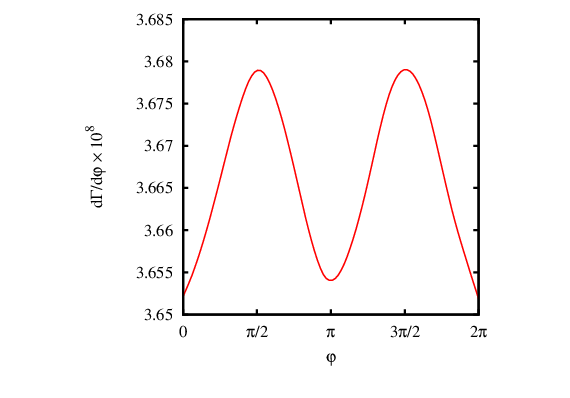
In figure 3 we have shown the plot of the differential branching ratio as a function of the azimuthal angle between the planes ρ​K\rho K and ℓ+​ℓ−\ell^{+}\ell^{-}. And in our final plot we have shown the dependence of the differential branching ratio as a function of the scattering angle θℓ\theta_{\ell} in ℓ+​ℓ−\ell^{+}\ell^{-}, as defined in figure 1.

We should like to note, at this point, that for any new physics model that can be effectively absorbed by the “standard” set of Wilson coefficients in the effective Hamiltonian, our analytic results given in previous sections can be used to obtain the corresponding change in the angular correlations.

Refer to caption
Figure 3: The differential branching ratio as a function of the azimuthal angle ϕ\phi.

As one final remark we may integrate our differential decay rate over the final state hadrons to get the decay rate of the process B→K1​ℓ+​ℓ−B\rightarrow K_{1}\ell^{+}\ell^{-}. Note that by using our defintion of the form factors we can relate these to the ones for K∗​(890)K^{*}(890), under the substitutions V↔−AV\leftrightarrow-A and T↔T5T\leftrightarrow T_{5}, such that the corresponding decay rates are obtained easily (by means of this substitution). It is easily seen then that the location of the zero in the FB asymmetry of this integrated decay rate is the same as in the K∗​(890)K^{*}(890) case, with the numerical value of the form factors being different. However, though the zeroes can be related, the overall shape of the FB asymmetries could be different from B→K∗​(890)B\to K^{*}(890).

To conclude, the mode which we have studied above, within the SM level, can in principal be measured at present BB-factories. Various angular correlations of this mode can also be studied in future SuperB factories. The study of the various angular correlations in B→K1(→ρK)ℓ+ℓ−B\to K_{1}(\to\rho K)\ell^{+}\ell^{-} can provide us with a very useful cross-checking tool for the SM and possible new physics in b→s​ℓ+​ℓ−b\to s\ell^{+}\ell^{-} transitions. In this pursuit we have given the LEET form factors for B→K1​(1270)​ℓ+​ℓ−B\to K_{1}(1270)\ell^{+}\ell^{-}, which could be useful in not only testing the operator structure of the SM but also the existence of possible new physics beyond it.

Refer to caption
Figure 4: The differential branching ratio as a function of θℓ\theta_{\ell}.

Acknowledgments

The work of SRC is supported by the Department of Science & Technology (DST), India. SRC would also like to thank the Theory Division, KEK, for their local hospitality, where the part of this work was done. The work of NG is supported by JSPS under the grant no. P06043.

Appendix A The form factors

Firstly, it is important to note that the additional negative sign in equation (19) is due to the difference in our definition of ε\varepsilon, as compared to that of Cheng and Chua [3], Charles et al.[2] and Kim et al.[1]. Furthermore, note that the definitions of Cheng et al. are the same as that of Charles et al., but differ from that of Kim et al. by a sign, which can be taken into account by changing the sign in equation (19).

The form factors, as defined in Cheng et al. (for all the form factors except YB​3Y_{B3})[3], are:

F⁡(q2)=F⁡(0)1−a⁡(q2/mB2)+b​(q2/mB2)2.F(q^{2})=\frac{F(0)}{1-a(q^{2}/m_{B}^{2})+b(q^{2}/m_{B}^{2})^{2}}\,\,\,. (39)

For YB​3Y_{B3} we use [3]:

F⁡(q2)=F⁡(0)(1−q2/mB2)​(1−a⁡(q2/mB2)+b​(q2/mB2)2).F(q^{2})=\frac{F(0)}{\left(1-q^{2}/m_{B}^{2}\right)\left(1-a(q^{2}/m_{B}^{2})+b(q^{2}/m_{B}^{2})^{2}\right)}\,\,\,. (40)

The numerical values of the factors appearing in equation (22) and equation (23) are given in Table 1.

F F(0) a b
YA​1Y_{A1} 0.11 0.68 0.35
YA​3Y_{A3} 0.19 1.02 0.35
YB​1Y_{B1} 0.13 1.94 1.53
YB​3Y_{B3} - 0.07 1.93 2.33
Table 1: The form factors for the YAiY_{A_{i}} and YBiY_{B_{i}}[3].

Appendix B Input Parameters

mB=5.26m_{B}=5.26 GeV,   mK1=1.27m_{K_{1}}=1.27 GeV,    mb=4.8m_{b}=4.8 GeV,    mρ=0.77m_{\rho}=0.77 GeV,    mK=0.134m_{K}=0.134 GeV,

α=1129\alpha=\frac{1}{129},    GF=1.17×10⁻⁵G_{F}=1.17\times 10^{-5} GeV-2,    |Vt​b​Vt​s∗|=0.0385|V_{tb}V_{ts}^{*}|=0.0385,

C7=−0.3,and​C10=−4.6,C_{7}=-0.3,~~\mathrm{and}~~C_{10}=-4.6,

References

  • [1] C. S. Kim, Y. G. Kim, C. D. Lu and T. Morozumi, Phys. Rev. D 62, 034013 (2000) [arXiv:hep-ph/0001151].
  • [2] J. Charles, A. Le Yaouanc, L. Oliver, O. Pene and J. C. Raynal, Phys. Rev. D 60, 014001 (1999) [arXiv:hep-ph/9812358].
  • [3] H. Y. Cheng and C. K. Chua, Phys. Rev. D 69, 094007 (2004) [arXiv:hep-ph/0401141].
  • [4] L. Roca, J. E. Palomar and E. Oset, Phys. Rev. D 70, 094006 (2004) [arXiv:hep-ph/0306188].
  • [5] H. Yang et al., Phys. Rev. Lett. 94, 111802 (2005) [arXiv:hep-ex/0412039].
  • [6] Y. J. Kwon and J. P. Lee, Phys. Rev. D 71, 014009 (2005) [arXiv:hep-ph/0409133] ; G. Nardulli and T. N. Pham, Phys. Lett. B 623, 65 (2005) [arXiv:hep-ph/0505048] ; J. P. Lee, Phys. Rev. D 74, 074001 (2006) [arXiv:hep-ph/0608087].
  • [7] F. Kruger and L. M. Sehgal, Phys. Lett. B 380, 199 (1996) [arXiv:hep-ph/9603237].