Interference pattern of a long diffusive Josephson junction

Introduction - The supercurrent flowing through a tunnel junction between two superconductors is given by the well-known gauge invariant Josephson relation

where $\delta$ is the phase difference between the two superconductors. The Josephson effect is thus a beautiful tool to exhibit interference effects, manifestations of the phase coherence of the superconducting wavefunction. For example, a circuit with two Josephson junctions is a realization of Young’s two slits experiment, where the interference is modulated by the Aharonov-Bohm flux through the circuit Mercereau64. Moreover a single Josephson junction with a finite width exhibits an interference pattern reminiscent of the diffraction (Fraunhofer) pattern of a slit, as recalled in eq. (4) Mercereau65.

It is natural to wonder whether such an interference experiment can probe phase coherence in a more complex medium with multiple scattering of the electrons. Here, we consider a long Josephson junction made of a diffusive metal forming a quasi-one-dimensional wire. The junction of length $L$ is attached to superconducting leads along the direction $x$. A magnetic field is applied along the direction $z$ perpendicular to the wire. The width of the junction (along the $y$ direction) is denoted by $w$, and its width (along $z$) is denoted by $h$. We consider a long junction such that $L\gg w$. The junction is schematically represented on figure 1. The amplitude of the Josephson current in such a diffusive junction has been calculated with the Usadel equation Belzig96; Heikkila02. It has been found that, contrary to the the case of the tunnel junction, for a good contact between the metallic region and the superconductors, the Josephson relation may not be sinusoidal. However, harmonics are expected to decay rapidly, roughly as $(-1)^{n}/n^{2}$. In this letter, we assume a sinusoidal Josephson relation and consider how the phase is modified by the application of a magnetic field. We find that for a long diffusive junction, the critical current varies as

where $\phi$ is the flux through the junction and $\phi_{0}=h/2e$ is the superconducting flux quantum.

Josephson current and diffusive trajectories - Quite generally, the Josephson current resulting from all current paths has the form

where $\langle\cdots\rangle_{\cal C}$ denotes the average over all current paths through the junction.

We choose a gauge where the vector potential ${\boldsymbol{A}}$ is aligned along the direction $x$, $A_{x}=By$, $y\in[-w/2,w/2]$. On figure 1, the diffuse paths $3-4$ represent current paths ${\cal C}$ while the straight path $1-2$ serves as a reference path and corresponds to $y=0$. The circulation of ${\boldsymbol{A}}$ is zero along the paths $1-2$, $1-3$ and $2-4$, so that the phase difference does not depend on $y$ and is denoted $\delta_{0}$. The current can be rewritten in the gauge dependent form

so that we write the critical current $I_{c}=\max[I(\delta)]$ as

or, in a gauge independent form:

$\phi({\cal C})$ is the flux through the area $1-3-4-2$ defined by a diffusive path ${\cal C}$. $\phi_{0}=h/2e$ is the superconducting flux quantum. We have neglected the current flowing in the superconductors along the $1-3$ and $2-4$ segments, i.e. we have assumed that the penetration length $\lambda$ of the magnetic field in the superconductor $\lambda\rightarrow 0$. Taking into account a finite $\lambda$ would amount to replace $L$ by $L+2\lambda$, as usual.

As a reminder, we first briefly consider the case of the short ballistic junction. The current has to be summed on the current paths

leading to the well-known Fraunhofer-like result Mercereau65

where $\phi=BwL$ (or $\phi=w(L+2\lambda)$ to account for a finite penetration length).

For a long diffusive junction, the phase factor in (3) has to be averaged on the distribution of diffusive trajectories. In order to perform this average, we need to describe the diffusion from a point ${\boldsymbol{r}}$ at one end of the diffusive sample to another point ${\boldsymbol{r}}^{\prime}$ located at the other end. We introduce the probability $P({\boldsymbol{r}},{\boldsymbol{r}}^{\prime},t)$, solution of the covariant equation

where the electron charge is denoted $-e$. This solution may be expressed as a functional integral Feynman :

We consider a long junction where the dephasing between ${\boldsymbol{r}}$ and ${\boldsymbol{r}}^{\prime}$ is supposed to be independent of the position of ${\boldsymbol{r}}$ and ${\boldsymbol{r}}^{\prime}$ on the boundaries, that is independent of the coordinates $y$ and $z$. Therefore, we consider a one-dimensional diffusion equation with the appropriate gauge:

from which we obtain the average $\langle\cdots\rangle_{{\cal C}}$ on diffusive trajectories

where $P_{0}$ is solution of eq. (7) with $B=0$, and $x$, $x^{\prime}$ are taken at the extremities of the junction. Then the critical current is obtained from eq. (3).

We solve this equation with the magnetic field as a perturbation. The eigenvalues of this diffusion equation are solutions of

and are given by

The new magnetic field dependent term implies an exponential decay of the probability $P(x,x^{\prime},t)=P_{0}(x,x^{\prime},t)e^{-t/\tau_{B}}$, with the characteristic time $\tau_{B}$ given by AltAronov:

The average (8) over diffusive trajectories is thus related to the Laplace transform $P_{\gamma}({\boldsymbol{r}},{\boldsymbol{r}}^{\prime})=\int P_{0}({\boldsymbol{r}},{\boldsymbol{r}}^{\prime},t)e^{-\gamma t}dt$ of the probability to diffuse from one end to the sample to the other. The numerator is the solution of the differential equation:

with $\gamma=1/\tau_{B}$, and with the appropriate boundary conditions. Here we assume that the disordered junction is connected to reservoirs and express that the probability vanishes at the edge of the diffusive metal (different boundary conditions could be discussed, but lead also to the same $1/\sinh L/L_{B}$ of eq. (15)). The solution of this equation is Montambaux04

where $x_{m}=\mbox{min}(x,x^{\prime})$ and $x_{m}=\mbox{max}(x,x^{\prime})$. We have introduced the characteristic length:

The coordinates $x$ and $x^{\prime}$ are close to the end of the diffusive junction. Their value is respectively $l$ and $L-l$ where the length $l$ is of the order of the elastic mean free path $l_{e}$ AM2. Since $l\ll L$, we obtain

In the limit $L_{B}\rightarrow\infty$, the probability scales as $1/L$ which expresses Ohm’s law that the transmission coefficient of a diffusive system scales like the inverse of its length. Now, from (14) and (8), we obtain finally a result independent of $l$:

that we write in the final form (2) where $\phi=BwL$ is the flux through the junction.

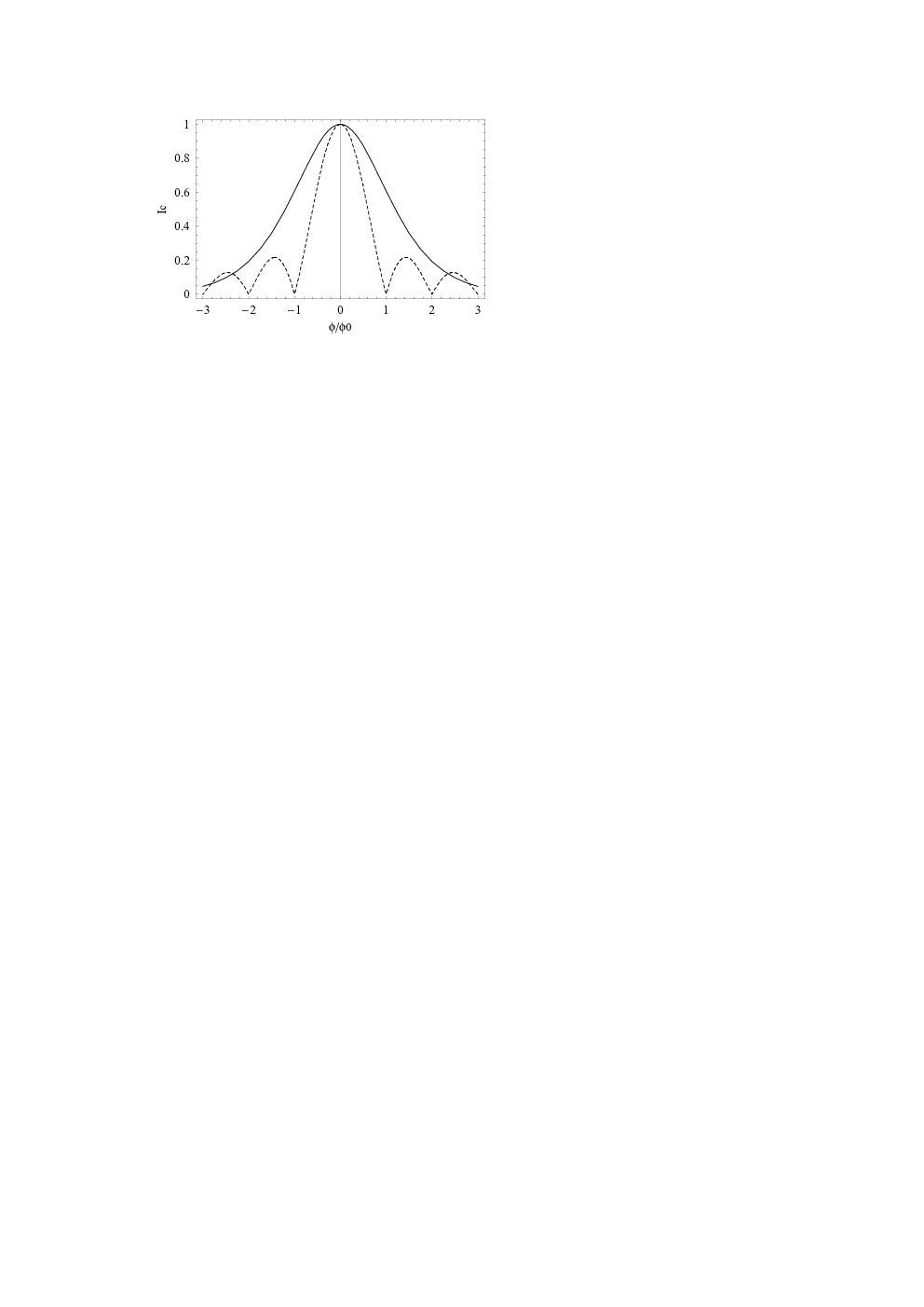
Phase coherence - This result assumes full phase coherence in the metallic junction. We now introduce a finite coherence time $\tau_{\phi}$ and the probability $P_{\gamma}(x,x^{\prime})$ is now solution of eq. (12) with $\gamma=1/\tau_{B}+1/\tau_{\phi}$. We immediately obtain

where $1/L_{\gamma}^{2}=1/L_{B}^{2}+1/L_{\phi}^{2}$ and $L_{\phi}=\sqrt{D\tau_{\phi}}$ is the phase coherence length. Similarly, the effect of a finite temperature can be taken into account by the thermal length $L_{T}=\sqrt{D/T}$, so that $1/L_{B}^{2}$ is replaced by $1/L_{B}^{2}+1/L_{T}^{2}$.

Gaussian accumulation of the phase - We now try to give a simple interpretation of our result. The dephasing accumulated along diffusive trajectories is characterized by the average $\langle e^{-i\varphi}\rangle_{\cal C}$ of the phase factor $\varphi={2\pi\over\phi_{0}}\int{\boldsymbol{A}}\cdot d{\boldsymbol{l}}$ along all diffusive paths ${\cal C}$ in the junction. Since diffusion is a Gaussian process, the average over trajectories of a given length, that is of a given diffusion time $t$, is

For a quasi-one-dimensional diffusion, the average $\langle\varphi_{t}^{2}\rangle_{\cal C}$ is simply given by $\langle\varphi_{t}^{2}\rangle_{\cal C}={4\pi^{2}\over\phi_{0}^{2}}{\overline{A^{2}}}\langle x_{t}^{2}\rangle_{\cal C}$, where $\overline{A^{2}}$ is an average taken along the transverse direction. Since $\overline{A^{2}}=B^{2}w^{2}/12$ and $\langle x_{t}^{2}\rangle_{\cal C}=2Dt$, we immediately obtain that the phase factor averaged along all trajectories of time $t$ is $\langle e^{-i\varphi_{t}}\rangle_{\cal C}=e^{-t/\tau_{B}}$ where $\tau_{B}$ has been defined in (11). Then the dephasing has to be averaged over all times $t$ for trajectories crossing the sample ($x\sim l,x^{\prime}\sim L-l$)

which is nothing but eq. (8).

Relation with weak localization - The magnetic field dependence of the Josephson current probes the phase accumulated along diffusive trajectoires which cross the sample. This physics bears of course some similarity with the weak localization correction which probes the distribution of dephasing along closed trajectories. Instead of probing the probability to cross the sample $P_{\gamma}(l,L-l)$, the weak localization correction probes the return probability $P_{\gamma}(x,x)$. As a result, for large $L\gg L_{B}$, the weak localization correction to the dimensionless conductance (in units of $2e^{2}/h$) decays as $1/L$.

while in the same limit $L\gg L_{B}$, the Josephson current decays exponentially

This behavior is very reminiscent of the structure of the harmonics of the weak localization correction on a ring as $e^{-mL/L_{B}}$ (the so-called Alsthuler-Aronov-Spivak oscillations AAS). It is a signature of the Gaussian decay of the probability to diffuse from one end to another after a time $t$, which scales as $e^{-L^{2}/4Dt}$. That is why the weak localization correction ($0^{th}$-harmonics) is a power law while the $m\neq 0$ harmonics decay exponentially. In the case of the ring, the boundary conditions are periodic along the ring, leading to the $e^{-mL/L_{B}}$ decay of the harmonics. Here, the trajectories can diffuse $m$ times back-and-forth before leaving the sample, leading to contributions of the form $e^{-(2m+1)L/L_{B}}$. The $1/\sinh L/L_{B}$ behavior results obviously from the additive contributions of these diffusive trajectories : $1/\sinh L/L_{B}=\sum_{m}e^{-(2m+1)L/L_{B}}$.

Relation with experiments in optics - Diffusing Wave Spectroscopy - The Josephson relation (1) involves the transmission coefficient of Cooper pairs which carry random phase factors that have to be averaged over diffusive trajectories. It is interesting to notice a similarity between our result for the diffusive Josephson junction and some results obtained in the physics of speckle correlations in optics. In optics, the so-called Diffusing Wave Spectroscopy (DWS) is a technique consisting in measuring the correlation function of the transmission amplitude $t$ of light through a turbid medium, measured at different times $0$ and $T$ DWS. If the scatterers of the diffusive medium can move, the correlation function gives some information on the motion on the dynamics of the scatterers.

The product $\langle t(0)t^{*}(T)\rangle$ involves pairings of diffusive trajectories which carry slightly different phases, since the scatterers have moved. Therefore it measures an average phase factor:

The phase accumulated along diffusive trajectories depends on the dynamics of the scatterers. For example, for a Brownian motion of the scatterers, the phase factor accumulated along trajectories of time $t$ decays exponentially, $\langle e^{-i\varphi_{t}}\rangle_{\cal C}=e^{-t/\tau_{\gamma}}$, where the characteristic dephasing time $\tau_{\gamma}$ depends on the ratio between the wave length $\lambda$ of the incident light beam and the typical displacement $\sqrt{D_{b}T}$ of the scatterers after time $T$. It has the form $\tau_{\gamma}\simeq\tau_{e}\lambda^{2}/D_{b}T$, where $\tau_{e}$ its elastic mean path and $D_{b}$ is the diffusion coefficient for the Brownian motion of the scatterers. Consequently the phase factor averaged over all trajectories which cross the sample is obtained from (17) and has the same decay (16) as found here for the diffusive Josephson junction in a field. Angular and frequency speckle correlations (the so-called $C_{1}$ correlations) exhibit a similar behavior Montambaux04; berkovits. The common physical origin is the Gaussian accumulation of the phase along diffusive trajectories.

Conclusion - comparison with experiments - Surprisingly, experiments on diffusive long diffusive $SNS$ junctions are pretty recent, the difficulty being of keeping phase coherence along the junction dubos. A recent experiment have measured the interference between two metallic $Au$ long junctions sandwiched in a superconducting $Al$ circuit Chiodi07. The total current oscillates with the flux through the circuit which modulates the relative phase between the junctions. This interference pattern is modulated by the interference pattern of each junction. This modulation is well described by our result. The low field behavior is very well fitted without adjustable parameter by the expansion $I_{c}=I_{0}(1-{\pi^{2}\over 18}{\phi^{2}\over\phi_{0}^{2}})+\cdots$ of our result (2). At large field however, the decay seems to be faster than exponential.

During the completion of this work, we have been aware of a preprint by Hammer et al. who consider the critical current of a long diffusive junction, within the Usadel formalism. For the case of a perfect transmission at the NS interface, they find for large $L/L_{B}$ an exponential decay of the form $L/L_{B}e^{-L/L_{B}}$ which is compatible with our equation (15) but they have considered only numerically the full range of magnetic field Cuevas07. Another paper Barzykin solves Usadel equation in the limit $L\gg L_{T}$.

Acknowlegments - The author acknowledges useful discussions with L. Angers, M. Aprili, H. Bouchiat, F. Chiodi, J.C. Cuevas, S. Guéron and M. Ferrier.

References

- (1) R.C. Jaklevic, J. Lambe, A.H. Silver and J.E. Mercereau, Phys. Rev. Lett. 12, 159 (1964).
- (2) R.C. Jaklevic, J. Lambe, J.E. Mercereau and A.H. Silver, Phys. Rev. 140, A1628 (1965).
- (3) W. Belzig, C. Bruder and G. Schön, Phys. Rev. B 54, 9443 (1996).
- (4) T.T. Heikkilä, J. Särkkä and F.K. Wilhelm, Phys. Rev. B 66, 184513 (2002).
- (5) É. Akkermans and G. Montambaux, Mesoscopic physics of electrons and photons, Cambridge University Press (2007).
- (6) R.P. Feynman and A.R. Hibbs, Quantum mechanics and path integrals, McGraw-Hill, New-York (1965); G. Roepstorff, Path integral approach to quantum physics: an introduction, Springer Verlag, New-York (1994).
- (7) B.L. Altshuler and A.G. Aronov, J.E.T.P. Lett. 33, 499 (1981).
- (8) A careful calculation for an interface with a ballistic medium gives Montambaux04.
- (9) B.L. Altshuler, A.G. Aronov and B.Z. Spivak, JETP Lett. 33, 94 (1981).
- (10) G. Maret and P.E. Wolf, Z. Phys. B 65, 409 (1987); D.J. Pine, D.A. Weitz, P.M. Chaikin and E. Herbolzheimer, Phys. Rev. Lett. 60, 1134 (1988). The quantity actually measured experimentally is the correlation function of intensities and at different times. It is simply related to the correlation function , see for example ref. Montambaux04.
- (11) R. Berkovits and S. Feng, Phys. Rep. 238, 135 (1994).
- (12) P. Dubos, H. Courtois, B. Pannetier, A.D. Wilhelm, A.D. Zaikin and G. Schön, Phys. Rev. B 63, 064502 (2001)
- (13) F. Chiodi, H. Bouchiat, S. Guéron, L. Angers, M. Ferrier, in preparation.
- (14) J.C. Hammer, J.C. Cuevas, F.S. Bergeret and W. Belzig, arXiv:0704.2358.
- (15) V. Barzykin and A.M. Zagoskin, Superlattices and Microstructures, 25, 797 (1999)