Width and finite extinction time of Ricci flowThanks: The authors were partially supported by NSF Grants DMS 0606629 and DMS 0405695
0. Introduction
This is an expository article with complete proofs intended for a general non-specialist audience. The results are two-fold. First, we discuss a geometric invariant, that we call the width, of a manifold and show how it can be realized as the sum of areas of minimal -spheres. For instance, when is a homotopy -sphere, the width is loosely speaking the area of the smallest -sphere needed to “pull over” . Second, we use this to conclude that Hamilton’s Ricci flow becomes extinct in finite time on any homotopy -sphere. We have chosen to write this since the results and ideas given here are quite useful and seem to be of interest to a wide audience.
Given a Riemannian metric on a closed manifold , sweep out by a continuous one-parameter family of maps from to starting and ending at point maps. Pull the sweepout tight by, in a continuous way, pulling each map as tight as possible yet preserving the sweepout. We show the following useful property (see Theorem 1.4 below); cf. 12.5 of [Al], proposition 3.1 of [Pi], proposition 3.1 of [CD], [CM3], and [CM1]:
Each map in the tightened sweepout whose area is close to the width (i.e., the maximal energy of the maps in the sweepout) must itself be close to a collection of harmonic maps. In particular, there are maps in the sweepout that are close to a collection of immersed minimal -spheres.
This useful property that all almost maximal slices are close to critical points is virtually always implicit in any sweepout construction of critical points for variational problems yet it is not always recorded since most authors are only interested in existence of a critical point.
Similar results hold for sweepouts by curves11 1 Finding closed geodesics on the -sphere by using sweepouts goes back to Birkhoff in 1917; see [B1], [B2], section in [Cr], and [CM3]. In the 1980s Sacks-Uhlenbeck, [SaU], found minimal -spheres on general manifolds using Morse theoretic arguments that are essentially equivalent to sweepouts; a few years later, Jost explicitly used sweepouts to obtain minimal -spheres in [Jo]. The argument given here works equally well on any closed manifold, but only produces non-trivial minimal objects when the width is positive. instead of -spheres; cf. [CM3] where sweepouts by curves are used to estimate the rate of change of a -dimensional width for convex hypersurfaces in Euclidean space flowing by positive powers of their mean curvatures. The ideas are essentially the same whether one sweeps out by curves or -spheres, though the techniques in the curve case are purely ad hoc whereas for sweepouts by -spheres additional techniques, developed in the 1980s, have to be used to deal with energy concentration (i.e., “bubbling”); cf. [SaU] and [Jo]. The basic idea in each of the two cases is a local replacement process that can be thought of as a discrete gradient flow. For curves, this is now known as Birkhoff’s curve shortening process; see [B1], [B2].
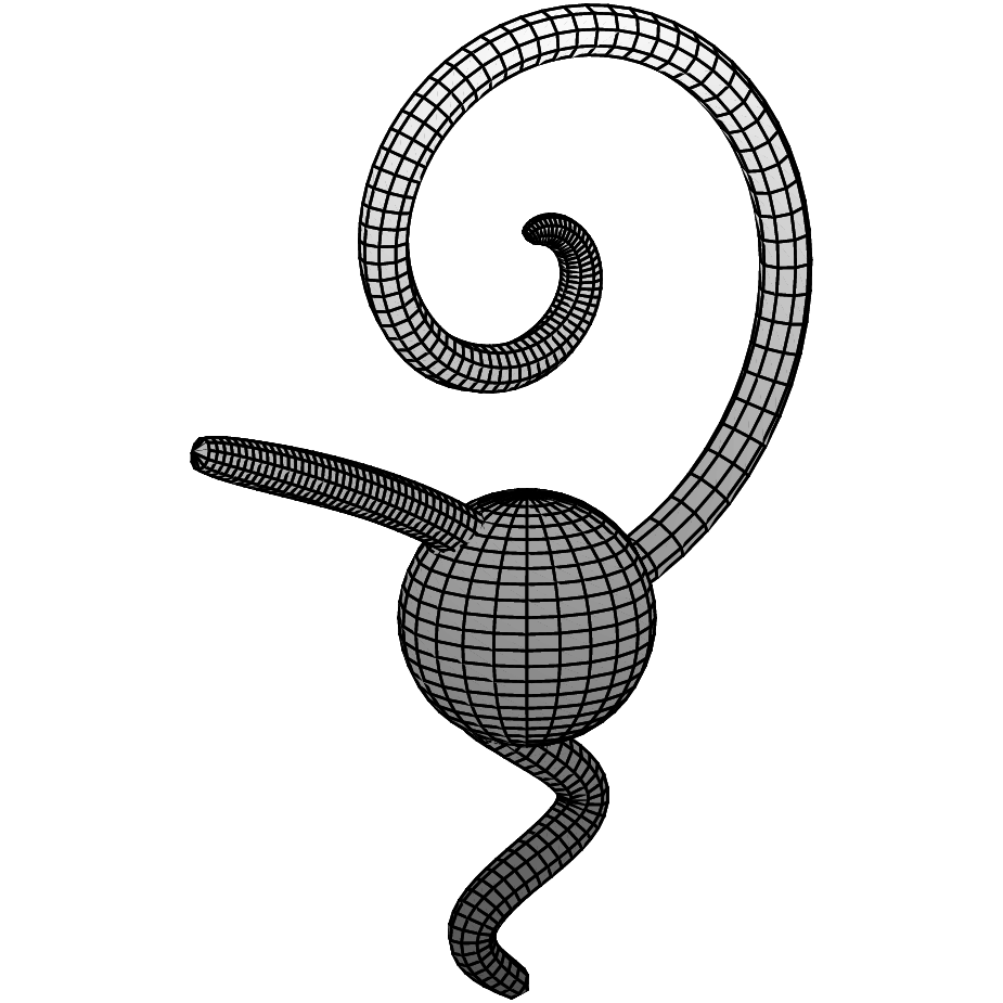
Local replacement had already been used by H.A. Schwarz in 1870 to solve the Dirichlet problem in general domains, writing the domain as a union of overlapping balls, and using that a solution can be found explicitly on balls by, e.g., the Poisson formula; see [Sc1] and [Sc2]. His method, which is now known as Schwarz’s alternating method, continues to play an important role in applied mathematics, in part because the replacements converge rapidly to the solution. The underlying reason why both Birkhoff’s method of finding closed geodesics and Schwarz’s method of solving the Dirichlet problem converge is convexity. We will deviate slightly from the usual local replacement argument and prove a new convexity result for harmonic maps. This allows us to make replacements on balls with small energy, as opposed to balls with small oscillation. It is, in our view, much more natural to make the replacement based on energy and gives, as a bi-product, a new uniqueness theorem for harmonic maps since already in dimension two the Sobolev embedding fails to control the norm in terms of the energy; see Figure 2.
The second thing we do is explain how to use this property of the width to show that on a homotopy -sphere, or more generally closed -manifolds without aspherical summands, the Ricci flow becomes extinct in finite time. This was shown by Perelman in [Pe] and by Colding-Minicozzi in [CM1]; see also [Pe] for applications to the elliptic part of geometrization.
We would like to thank Frédéric Hélein, Bruce Kleiner, and John Lott for their comments.
1. Width and finite extinction
On a homotopy -sphere there is a natural way of constructing minimal surfaces and that comes from the min-max argument where the minimal of all maximal slices of sweepouts is a minimal surface. In [CM1] we looked at how the area of this min-max surface changes under the flow. Geometrically the area measures a kind of width of the -manifold (see Figure 2) and for -manifolds without aspherical summands (like a homotopy -sphere) when the metric evolve by the Ricci flow, the area becomes zero in finite time corresponding to that the solution becomes extinct in finite time.22 2 It may be of interest to compare our notion of width, and the use of it, to a well-known approach to the Poincaré conjecture. This approach asks to show that for any metric on a homotopy -sphere a min-max type argument produces an embedded minimal -sphere. Note that in the definition of the width it play no role whether the minimal -sphere is embedded or just immersed, and thus, the analysis involved in this was settled a long time ago. This well-known approach has been considered by many people, including Freedman, Meeks, Pitts, Rubinstein, Schoen, Simon, Smith, and Yau; see [CD].
1.1. Width
Let be the set of continuous maps so that for each the map is in , the map is continuous from to , and finally maps and to points. Given a map , the homotopy class is defined to be the set of maps that are homotopic to through maps in . We will call any such a sweepout; some authors use a more restrictive notion where must also induce a degree one map from to . We will, in fact, be most interested in the case where induces a map from to in a non-trivial class33 3 For example, when is a homotopy -sphere and the induced map has degree one. in . The reason for this is that the width is positive in this case and, as we will see, equal to the area of a non-empty collection of minimal -spheres.
The (energy) width associated to the homotopy class is defined by taking the infimum of the maximum of the energy of each slice. That is, set
| (1.1) |
where the energy is given by
| (1.2) |
Even though this type of construction is always called min-max, it is really inf-max. That is, for each (smooth) sweepout one looks at the maximal energy of the slices and then takes the infimum over all sweepouts in a given homotopy class. The width is always non-negative by definition, and positive when the homotopy class of is non-trivial. Positivity can, for instance, be seen directly using [Jo]. Namely, page 125 in [Jo] shows that if is sufficiently small (depending on ), then is homotopically trivial.44 4 See the remarks after Corollary 3.2 for a different proof.
One could alternatively define the width using area rather than energy by setting
| (1.3) |
The area of a map is by definition the integral of the Jacobian , where is the differential of and is its transpose. That is, if is an orthonormal frame on , then and
| (1.4) |
Consequently, area is less than or equal to energy with equality if and only if and are zero (as functions). In the case of equality, we say that is almost conformal. As in the classical Plateau problem (cf. Section 4 of [CM2]), energy is somewhat easier to work with in proving the existence of minimal surfaces. The next proposition, proven in Appendix D, shows that as for the Plateau problem (clearly, by the discussion above). Therefore, we will drop the subscript and just write .
Proposition \the\fnum.
.
1.2. Finite extinction
Let be a smooth closed orientable -manifold and a one-parameter family of metrics on evolving by Hamilton’s Ricci flow, [Ha1], so
| (1.5) |
When is prime and non-aspherical, then it follows by standard topology that is non-trivial (see, e.g., [CM1]). For such an , fix a non-trivial homotopy class . It follows that the width is positive for each metric . This positivity is the only place where the assumption on the topology of is used in the theorem below giving an upper bound for the derivative of the width under the Ricci flow. As a consequence, we get that the solution of the flow becomes extinct in finite time (see paragraph 4.4 of [Pe] for the precise definition of extinction time when surgery occurs).
Theorem \the\fnum.
[CM1]. Let be a closed orientable prime non-aspherical -manifold equipped with a metric . Under the Ricci flow, the width satisfies
| (1.6) |
in the sense of the limsup of forward difference quotients. Hence, becomes extinct in finite time.
The in (1.6) comes from the Gauss-Bonnet theorem and the comes from the bound on the minimum of the scalar curvature that the evolution equation implies. Both of these constants matter whereas the constant depends on the initial metric and the actual value is not important.
To see that (1.6) implies finite extinction time rewrite (1.6) as
| (1.7) |
and integrate to get
| (1.8) |
Since by definition and the right hand side of (1.8) would become negative for sufficiently large, we get the claim.
Theorem 1.2 shows, in particular, that the Ricci flow becomes extinct for any homotopy -sphere. In fact, we get as a corollary finite extinction time for the Ricci flow on all -manifolds without aspherical summands (see of [Pe] or section of [CM1] for why this easily follows):
Corollary \the\fnum.
Part of Perelman’s interest in the question about finite time extinction comes from the following: If one is interested in geometrization of a homotopy -sphere (or, more generally, a -manifold without aspherical summands) and knew that the Ricci flow became extinct in finite time, then one would not need to analyze what happens to the flow as time goes to infinity. Thus, in particular, one would not need collapsing arguments.
One of the key ingredients in the proof of Theorem 1.2 is the existence of a sequence of good sweepouts of , where each map in the sweepout whose area is close to the width (i.e., the maximal energy of any map in the sweepout) must itself be close to a collection of harmonic maps. This will be given by Theorem 1.4 below, but we will first need a notion of closeness and a notion of convergence of maps from into a manifold.
1.3. Varifold convergence
Fix a closed manifold and let be the Grassmanian bundle of (un-oriented) -planes, that is, each fiber is the set of all -dimensional linear subspaces of the tangent space of at . Since is compact, we can choose a countable dense subset of all continuous functions on with supremum norm at most one (dense with respect to the supremum norm).55 5 This is a corollary of the Stone-Weierstrass theorem; see corollary on page of [R]. If and are two compact (not necessarily connected) surfaces , with measurable maps so that each is in and is the Jacobian of , then the varifold distance between them is by definition
| (1.9) |
It follows easily that a sequence with uniformly bounded areas converges to , iff it converges weakly, that is, if for all we have . For instance, when is a -manifold, then , , and are isomorphic. (Here is the unit tangent bundle.) If is a sequence of closed immersed surfaces in converging to a closed surface in the usual topology, then we can think of each surface as being embedded in by mapping each point to plus-minus the unit normal vector, , to the surface. It follows easily that the surfaces with these inclusion maps converges in the varifold distance. More generally, if is a compact surface and is a map, where is no longer assumed to be -dimensional, then we let be given by that is the linear subspace . (When is -dimensional, then we may think of the image of this map as lying in .) Strictly speaking, this is only defined on the measurable space, where is non-zero; we extend it arbitrarily to all of since the corresponding Radon measure on given by is independent of the extension.
1.4. Existence of good sweepouts
A map on a smooth compact surface with boundary is energy minimizing to if is in for almost every and
| (1.10) |
The map is said to be weakly harmonic if is a weak solution of the harmonic map equation ; see, e.g., lemma in [He1].
The next result gives the existence of a sequence of good sweepouts.
Theorem \the\fnum.
Given a metric on and a map representing a non-trivial class in , there exists a sequence of sweepouts with , and so that given , there exist and so that if and
| (1.11) |
then there are finitely many harmonic maps with
| (1.12) |
One immediate consequence of Theorem 1.4 is that if is any sequence with converging to the width as , then a subsequence of converges to a collection of harmonic maps from to . In particular, the sum of the areas of these maps is exactly and, since the maps are automatically conformal, the sum of the energies is also . The existence of at least one non-trivial harmonic map from to was first proven in [SaU], but they allowed for loss of energy in the limit; cf. also [St]. This energy loss was ruled out by Siu and Yau, using also arguments of Meeks and Yau (see Chapter VIII in [SY]). This was also proven later by Jost in theorem of [Jo] which gives at least one min-max sequence converging to a collection of harmonic maps. The convergence in [Jo] is in a different topology that, as we will see in Appendix A, implies varifold convergence.
1.5. Upper bounds for the rate of change of width
Throughout this subsection, let be a smooth closed prime and non-aspherical orientable -manifold and let be a one-parameter family of metrics on evolving by the Ricci flow. We will prove Theorem 1.2 giving the upper bound for the derivative of the width under the Ricci flow. To do this, we need three things.
One is that the evolution equation for the scalar curvature , see page 16 of [Ha2],
| (1.13) |
implies by a straightforward maximum principle argument that at time
| (1.14) |
The curvature is normalized so that on the unit the Ricci curvature is and the scalar curvature is . In the derivation of (1.14) we implicitly assumed that . If this was not the case, then (1.14) trivially holds for any , since, by (1.13), is always non-decreasing. This last remark is also used when surgery occurs. This is because by construction any surgery region has large (positive) scalar curvature.
The second thing that we need in the proof is the observation that if is a collection of branched minimal -spheres and with , then for any smooth quadratic form on we have (the unit normal is defined where )
| (1.15) |
The last thing is an upper bound for the rate of change of area of minimal -spheres. Suppose that is a closed surface and is a map, then using (1.5) an easy calculation gives (cf. pages 38–41 of [Ha2])
| (1.16) |
If is a closed immersed minimal surface, then
| (1.17) |
Here is the (intrinsic) curvature of , is the second fundamental form of , and is the sum of the squares of the principal curvatures. To get (1.17) from (1.16), we used that if is the sectional curvature of on the two-plane tangent to , then the Gauss equations and minimality of give . The next lemma gives the upper bound.
Lemma \the\fnum.
If is a branched minimal immersion of the -sphere, then
| (1.18) |
Proof.
Let be the set of branch points of and the order of branching. By (1.17)
| (1.19) |
where the equality used the Gauss-Bonnet theorem with branch points (this equality also follows from the Bochner type formula for harmonic maps between surfaces given on page of [SY] and the second displayed equation on page of [SY] that accounts for the branch points). Note that branch points only help in the inequality (1.18). ∎
Using these three things, we can show the upper bound for the rate of change of the width.
Proof.
(of Theorem 1.2) Fix a time . Below denotes a constant depending only on but will be allowed to change from line to line. Let be the sequence of sweepouts for the metric given by Theorem 1.4. We will use the sweepout at time as a comparison to get an upper bound for the width at times . The key for this is the following claim: Given , there exist and so that if and , then
| (1.20) |
To see why (1.5) implies (1.6), use the equivalence of the two definitions of widths to get
| (1.21) |
and take the limit as (so that66 6 This follows by combining that by (1.4), , and by the equivalence of the two definitions of width. ) in (1.5) to get
| (1.22) |
It remains to prove (1.5). First, let and , depending on (and on ), be given by Theorem 1.4. If and , then let be the collection of minimal spheres given by Theorem 1.4. Combining (1.16), (1.15) with , and Lemma 1.5 gives
| (1.23) | ||||
where the last inequality used the lower bound (1.14) for . Since the metrics vary smoothly and every sweepout has uniformly bounded energy, it is easy to see that is a smooth function of with a uniform bound independent of both and near (cf. (1.16)). In particular, (1.5) and Taylor expansion give (independent of ) so that (1.5) holds for with . In the remaining case, we have so the continuity of implies that (1.5) automatically holds after possibly shrinking . ∎
1.6. Parameter spaces
Instead of using the unit interval, , as the parameter space for the maps in the sweepout and assuming that the maps start and end in point maps, we could have used any compact finite dimensional topological space and required that the maps are constant on (or that ). In this case, let be the set of continuous maps so that for each the map is in , the map is continuous from to , and finally maps to point maps. Given a map , the homotopy class is defined to be the set of maps that are homotopic to through maps in . Finally, the width is . With only trivial changes, the same proof yields Theorem 1.4 for these general parameter spaces.77 7 The main change is in Lemma 3.4 below where the bound for the multiplicity in (1) becomes . This follows from the definition of (covering) dimension; see pages and in [Mu].
2. The energy decreasing map and its consequences
To prove Theorem 1.4, we will first define an energy decreasing map from to itself that preserves the homotopy class (i.e., maps each to itself) and record its key properties. This should be thought of as a generalization of Birkhoff’s curve shortening process that plays a similar role when tightening a sweepout by curves; see [B1], [B2], [Cr], and [CM3].
Throughout this paper, by a ball , we will mean a subset of and a stereographic projection so that is a ball. Given , we will let denote of the ball with the same center as and radius times that of .
Theorem \the\fnum.
There is a constant and a continuous function with , both depending on , so that given any without non-constant harmonic slices and , there exists so that for each and so for each with :
- ()
If is any finite collection of disjoint closed balls in with and is an energy minimizing map equal to on , then
The proof of Theorem 2 is given in Section 3. The second ingredient that we will need to prove Theorem 1.4 is a compactness result that generalizes compactness of harmonic maps to maps that are closer and closer to being harmonic (this is Proposition 2.1 below and will be proven in Appendix B).
2.1. Compactness of almost harmonic maps
Our notion of almost harmonic relies on two important properties of harmonic maps from to . The first is that harmonic maps from are conformal and, thus, energy and area are equal; see (A) below. The second is that any harmonic map from a surface is energy minimizing when restricted to balls where the energy is sufficiently small; see (B) below.
In the proposition, (depending on ) is the small energy constant from lemma in [SaU], so that we get interior estimates for harmonic maps with energy at most . In particular, any non-constant harmonic map from to has energy greater than .
Proposition \the\fnum.
Suppose that are constants with
and
is a sequence of maps with
satisfying:
(A) .
(B) For any finite collection of disjoint closed
balls in with there is an
energy minimizing
map that equals on with
If (A) and (B) are satisfied, then a subsequence of the ’s varifold converges to a collection of harmonic maps .
One immediate consequence of Proposition 2.1 is a compactness theorem for sequences of harmonic maps with bounded energy. This was proven by Jost in lemma in [Jo]. In fact, Parker proved compactness of bounded energy harmonic maps in a stronger topology, with convergence in addition to convergence; see theorem in [Pa]. Therefore, it is perhaps not surprising that a similar compactness holds for sequences that are closer and closer to being harmonic in the sense above. However, it is useful to keep in mind that Parker has constructed sequences of maps where the Laplacian is going to zero in and yet there is no convergent subsequence (see proposition in [Pa]).
Finally, we point out that Proposition 2.1 can be thought of as a discrete version of Palais-Smale Condition (C). Namely, if we have a sequence of maps where the maximal energy decrease from harmonic replacement goes to zero, then a subsequence converges to a collection of harmonic maps.
2.2. Constructing good sweepouts from the energy decreasing map on
Given Theorem 2 and Proposition 2.1, we will prove Theorem 1.4. Let be the set of collections of harmonic maps from to so that the sum of the energies is at most .
Proof.
(of Theorem 1.4.) Choose a sequence of maps with
| (2.1) |
and so that is not harmonic unless it is a constant map.88 8 To do this, first use Lemma D.1 (density of -sweepouts) to choose so is continuous from to and . Using stereographic projection, we can view as a map from . Now fix a . The continuity in gives a uniform bound for some . Choose with . Define a map in polar coordinates by: for , for , and for . Note that is homotopic to the identity, is conformal away from the annulus , and on has and . It follows that is in , satisfies (2.1), and has on . Since harmonic maps from are conformal (corollary in [SaU]), any harmonic is constant on and, thus, constant on by unique continuation (theorem in [Sj]). We can assume that since otherwise and the theorem follows trivially.
Applying Theorem 2 to the ’s gives a sequence where each has energy at most that of . We will argue by contradiction to show that the ’s have the desired property. Suppose, therefore, that there exist and with and . Thus, by (2.1) and the fact that , we get
| (2.2) |
and, similarly, .
Using (2.2) in Theorem
2 gives
(B) If is any collection of disjoint
closed balls in with and is an
energy minimizing
map that equals on , then
| (2.3) |
Therefore, we can apply Proposition 2.1 to get that a subsequence of the ’s varifold converges to a collection of harmonic maps. However, this contradicts the lower bound for the varifold distance to , thus completing the proof. ∎
3. Constructing the energy decreasing map
3.1. Harmonic replacement
The energy decreasing map from to itself will be given by a repeated replacement procedure. At each step, we replace a map by a map that coincides with outside a ball and inside the ball is equal to an energy-minimizing map with the same boundary values as . This is often referred to as harmonic replacement.
One of the key properties that makes harmonic replacement useful is that the energy functional is strictly convex on small energy maps. Namely, Theorem 3.1 below gives a uniform lower bound for the gap in energy between a harmonic map and a map with the same boundary values; see Appendix C for the proof.
Theorem \the\fnum.
There exists a constant (depending on ) so that if and are maps from to , and agree on , and is weakly harmonic with energy at most , then
| (3.1) |
An immediate corollary of Theorem 3.1 is uniqueness of solutions to the Dirichlet problem for small energy maps (and also that any such harmonic map minimizes energy).
Corollary \the\fnum.
Let be as in Theorem 3.1. If and are weakly harmonic maps from to , both with energy at most , and they agree on , then .
3.2. Continuity of harmonic replacement on
The second consequence of Theorem 3.1 is that harmonic replacement is continuous as a map from to itself if we restrict to small energy maps. (The norm on is the sum of the sup norm and the norm.)
Corollary \the\fnum.
Let be as in Theorem 3.1 and set
| (3.2) |
Given , there is a unique energy minimizing map equal to on and is in . Furthermore, there exists depending on so that if with corresponding energy minimizing maps , and we set , then
| (3.3) |
Finally, the map from to is continuous as a map from to itself.
In the proof, we will use that since is smooth, compact and embedded, there exists a so that for each in the -tubular neighborhood of in , there is a unique closest point and so the map is smooth. is called nearest point projection. Furthermore, for any , we have . Therefore, there is a constant depending on so that for any , we have . In particular, we can choose so that for any and .
Proof.
(of Corollary 3.2.) The existence of an energy minimizing map was proven by Morrey in [Mo1]; by Corollary 3.1, is unique. The continuity of on is the main theorem of [Q].99 9 Continuity also essentially follows from the boundary regularity of Schoen and Uhlenbeck, [SU2], except that [SU2] assumes regularity of the boundary data. It follows that .
Step 1: is uniformly continuous. We can assume that , since (3.3) holds with if . Define a map by
| (3.4) |
so that maps to and agrees with on . Using that for and maps to , we can estimate the energy of by
| (3.5) |
where is the Lipschitz norm of in . Since and agree on , Corollary 3.1 yields . By symmetry, we can assume that so that (3.5) implies (3.3).
Step 2: The continuity of . Suppose that are in with in and and are the corresponding energy minimizing maps.
We will first show that in . To do this, set
| (3.6) |
so that maps to and agrees with on . Arguing as in (3.5) and using that by Step 1, we get that . Therefore, applying Theorem 3.1 to gives that . Since and , it follows that . The triangle inequality gives .
Finally, we will argue by contradiction to see that in . Suppose instead that there is a subsequence (still denoted ) with
| (3.7) |
Using the uniform energy bound for the ’s together with interior estimates for energy minimizing maps of [SU1] (and the Arzela-Ascoli theorem), we can pass to a further subsequence so that the ’s converge uniformly in on any compact subset . Finally, as remarked in the proof of the main theorem in [Q], proposition and remark of [Q] imply that the ’s are also equicontinuous near , so Arzela-Ascoli gives a further subsequence that converges uniformly on to a harmonic map that agrees with on the boundary. However, (3.7) implies that which contradicts the uniqueness of small energy harmonic maps. This completes the proof. ∎
Corollary 3.2 gives another proof that the width is positive when the homotopy class is non-trivial or, equivalently, that if is sufficiently small (depending on ), then is homotopically trivial. Namely, since is continuous from to , we can choose so that maps the ball into a convex geodesic ball in for every . If each has energy less than given by Corollary 3.2, then replacing outside by the energy minimizing map with the same boundary values gives a homotopic sweepout . Moreover, the entire image of is contained in the convex ball by the maximum principle.1010 10 This follows from lemma in [Jo] which requires that is homotopic to a map in and this follows from the small energy bound and the uniform lower bound for the energy of any homotopically non-trivial map from given, e.g., in the first line of the proof of proposition on page of [SY]. It follows that is homotopically trivial by contracting each to the point via a geodesic homotopy.
3.3. Uniform continuity of energy improvement on
It will be convenient to introduce some notation for the next lemma. Namely, given a map from to and a finite collection of disjoint closed balls in so the energy of on is at most , let denote the map that coincides with on and on is equal to the energy minimizing map from to that agrees with on . To keep the notation simple, we will set . Finally, if , then will denote the collection of concentric balls but whose radii are shrunk by the factor .
In general, is not the same as . This matters in the proof of Theorem 2, where harmonic replacement on either or decreases the energy of by a definite amount. The next lemma (see (3.8)) shows that the energy goes down a definite amount regardless of the order that we do the replacements. The second inequality bounds the possible decrease in energy from applying harmonic replacement on in terms of the possible decrease from harmonic replacement on .
Lemma \the\fnum.
There is a constant (depending on ) so that if is in and , are each finite collections of disjoint closed balls in so that the energy of on each is at most , then
| (3.8) |
Furthermore, for any , we have
| (3.9) |
We will prove Lemma 3.3 by constructing comparison maps with the same boundary values and using the minimizing property of small energy harmonic maps to get upper bounds for the energy. The following lemma will be used to construct the comparison maps.
Lemma \the\fnum.
There exists (depending on ) so that if are maps that agree at one point and satisfy
| (3.10) |
then there exists some and a map so that
| (3.11) |
and .
Proof.
Let and (depending on ) be as in the proof of Corollary 3.2 and set . Since vanishes somewhere on , integrating (3.10) gives .
Since the statement is scale-invariant, it suffices to prove the case . Set and define by
| (3.12) |
Observe that satisfies (3.11). Furthermore, since vanishes somewhere on , we can use Wirtinger’s inequality to bound by
| (3.13) | ||||
Since , the image of is contained in where we have . Therefore, if we set , then the energy of is at most twice the energy of . ∎
Proof.
(of Lemma 3.3.) We will index the balls in by and use for the balls in ; i.e., let and . The key point is that, by Corollary 3.2, small energy harmonic maps minimize energy. Using this, we get upper bounds for the energy of the harmonic replacement by cutting and pasting to construct comparison functions with the same boundary values.
Observe that the total energy of on the union of the balls in is at most . Since harmonic replacement on does not change the map outside these balls and is energy non-increasing, it follows that the total energy of on is at most .
The proof of (3.8). We will divide into two disjoint subsets, and , and argue separately, depending on which of these accounts for more of the decrease in energy after harmonic replacement. Namely, set
| (3.14) |
Since the balls in are disjoint, it follows that
| (3.15) |
Case 1. Suppose that . Since the balls in are contained in balls in and harmonic replacements minimize energy, we get
| (3.16) |
so that .
Case 2. Suppose now that
| (3.17) |
Let be given by Lemma 3.3. We can assume that
| (3.18) |
since otherwise Theorem 3.1 gives (3.8) with . The key is to show for that
| (3.19) | ||||
where is a universal constant. Namely, summing (3.19) over and using the inequality , the bound for the energy of in , and Theorem 3.1 to relate the energy of to gives
| (3.20) |
where we have set in the last line and the last inequality used that . Combining (3.17) with (3.20) gives (3.8).
To complete Case 2, we must prove (3.19). After translation, we can assume that is the ball of radius about in . Set and apply the co-area formula to get (in fact, a set of ’s of measure at least ) with
| (3.21) | ||||
| (3.22) |
Since and , the circle is not contained in any of the balls in . It follows that contains at least one point outside and, thus, there is a point in where . This and (3.18) allow us to apply Lemma 3.3 to get and a map with , , and
| (3.23) |
Observe that the map maps to and agrees with on . Therefore, the map from to which is equal to on , is equal to on , and is equal to on gives an upper bound for the energy of
| (3.24) |
Using (3.23) and that , we get
Since , we get (3.19).
The proof of (3.9). We will argue similarly with a few small modifications that we will describe. This time, let be the balls with contained in some . It follows that harmonic replacement on does not change and, thus,
| (3.25) |
Again, we can assume that (3.18) holds. Suppose now that . Arguing as in the proof of (3.19) (switching the roles of and ), we get
| (3.26) | ||||
Summing this over and arguing as for (3.20) gives
| (3.27) | ||||
3.4. Constructing the map from to
We will construct from by harmonic replacement on a family of balls in varying continuously in . The balls will be chosen in Lemma 3.4 below. Throughout this subsection, will be the small energy constant (depending on ) given by Theorem 3.1.
Given and , define the maximal improvement from harmonic replacement on families of balls with energy at most by
| (3.28) |
where the supremum is over all finite collections of disjoint closed balls where the total energy of on is at most . Observe that is nonnegative, monotone non-decreasing in , and is positive if is not harmonic.
Lemma \the\fnum.
If is not harmonic and , then there is an open interval containing so that for all in the double interval .
Proof.
By (3.3) in Corollary 3.2, there exists (depending on ) so that if
| (3.29) |
and is a finite collection of disjoint closed balls where both and have energy at most , then
| (3.30) |
Here we have used that since is not harmonic. Since is continuous as a map to , we can choose so that for all (3.29) holds and
| (3.31) |
Suppose now that and the energy of is at most on a collection . It follows from (3.31) that the energy of is at most on . Combining (3.30) and (3.31) gives
| (3.32) |
Since this applies to any such , we get that . ∎
Given a sweepout with no harmonic slices, the next lemma constructs finitely many collections of balls so that harmonic replacement on at least one of these collections strictly decreases the energy. In addition, each collection consists of finitely many pairwise disjoint closed balls.
Lemma \the\fnum.
If and has no non-constant harmonic slices, then we get an integer (depending on ), collections of balls in , and continuous functions so that for each :
- (1)
At most two ’s are positive and for each .
- (2)
If , then there exists so that harmonic replacement on decreases energy by at least .
Proof.
Since the energy of the slices is continuous in , the set is compact. For each , choose a finite collection of disjoint closed balls in with so
| (3.33) |
Lemma 3.4 gives an open interval containing so that for all
| (3.34) |
Using the continuity of in and Corollary 3.2, we can shrink so that has energy at most in for and, in addition,
| (3.35) |
Since is compact, we can cover by finitely many ’s, say . Moreover, after discarding some of the intervals, we can arrange that each is in at least one closed interval , each intersects at most two other ’s, and the ’s intersecting do not intersect each other.1111 11 We will give a recipe for doing this. First, if is contained in the union of two other intervals, then throw it out. Otherwise, consider the intervals whose left endpoint is in , find one whose right endpoint is largest and discard the others (which are anyway contained in these). Similarly, consider the intervals whose right endpoint is in and throw out all but one whose left endpoint is smallest. Next, repeat this process on (unless it has already been discarded), etc. After at most steps, we get the desired cover. For each , choose a continuous function so that
- •
on and is zero for .
- •
is zero on the intervals that do not intersect .
Property (1) follows directly and (2) follows from (3.33), (3.34), and (3.35). ∎
Proof.
(of Theorem 2). Let and be given by Lemma 3.4. We will use an step replacement process to define . Namely, first set and then, for each , define by applying harmonic replacement to on the -th family of balls ; i.e, set . Finally, we set .
A key point in the construction is that property (1) of the family of balls gives that only two ’s are positive for each . Therefore, the energy bound on the balls given by property (1) implies that each energy minimizing map replaces a map with energy at most . Hence, Corollary 3.2 implies that these depend continuously on the boundary values, which are themselves continuous in , so that the resulting map is also continuous in . Finally, it is clear that is homotopic to since continuously shrinking the disjoint closed balls on which we make harmonic replacement gives an explicit homotopy. Thus, as claimed.
For each with , property (2) of the family of balls gives some so that harmonic replacement for on decreases the energy by at least . Thus, even in the worst case where is the second family of balls that we do replacement on at , (3.8) in Lemma 3.3 gives
| (3.36) |
To establish (), suppose that is a finite collection of disjoint closed balls in so that the energy of on is at most . We can assume that has energy at most on for every since otherwise Theorem 3.1 implies a positive lower bound for . Consequently, we can apply (3.9) in Lemma 3.3 twice (first with and then with ) to get
| (3.37) |
Combining (3.36) and (3.4) with Theorem 3.1 gives () and, thus, completes the proof. ∎
Appendix A Bubble convergence implies varifold convergence
A.1. Bubble convergence and the topology on
We will need a notion of convergence for a sequence of maps to a collection of maps which is similar in spirit to the convergence in Gromov’s compactness theorem for pseudo holomorphic curves, [G]. The notion that we will use is a slight weakening of the bubble tree convergence developed by Parker and Wolfson for -holomorphic curves in [PaW] and used by Parker for harmonic maps in [Pa]. In our applications, the ’s will be approximately harmonic while the limit maps will be harmonic. We will need the next definition to make this precise.
and will denote the northern and southern hemispheres in and and the north and south poles.
Definition \the\fnum.
Given a ball , the conformal dilation taking to is the composition of translation followed by dilation of about taking to .
The standard example of a conformal dilation comes from applying stereographic projection , then dilating by a positive , and applying .
In the definition below of convergence, the map will be the standard -weak limit of the ’s (see (B1)), while the other ’s will arise as weak limits of the composition of the ’s with a divergent sequence of conformal dilations of (see (B2)). The condition (B3) guarantees that these limits all arise in genuinely distinct ways, and the condition (B4) means that together the ’s account for all of the energy.
Definition \the\fnum.
Bubble convergence. We will say that a sequence of maps converges to a collection of maps if the following hold:
- (B1)
The ’s converge weakly to in and there is a finite set so that the ’s converge strongly to in for any compact .
- (B2)
For each , we get a point and a sequence of balls with and . Furthermore, if is the conformal dilation taking the southern hemisphere to , then the maps converge to as in (B1). Namely, weakly in and there is a finite set so that the ’s converge strongly in for any compact .
- (B3)
If , then .
- (B4)
We get the energy equality .
A.2. Two simple examples of bubble convergence
The simplest non-trivial example of bubble convergence is when each map is the composition of a fixed harmonic map with a divergent sequence of dilations . In this case, the ’s converge to the constant map on each compact set of and all of the energy concentrates at the single point . Composing the ’s with the divergent sequence of conformal dilations gives the limit .
For the second example, let be stereographic projection and let be complex coordinates on . If we set , then the maps are conformal and, therefore, also harmonic. Since each is a rational map of degree two, we have . Moreover, the ’s converge away from to the identity map which has energy . The other of energy disappears at but can be accounted for by a map by composing with a divergent sequence of conformal dilations; must also have degree one. In this case, the conformal dilations take to which converges to the conformal inversion about the circle of radius one.
A.3. Bubble convergence implies varifold convergence
Proposition \the\fnum.
If a sequence of maps bubble converges to a finite collection of smooth maps , then it also varifold converges.
Before getting to the proof, recall that a sequence of functions is said to converge in measure to a function if for all the measure of goes to zero as ; see [R], page . Clearly, convergence implies convergence in measure. Furthermore, if in measure and is uniformly continuous, then in measure. Finally, we will use the following general version of the dominated convergence theorem which combines theorem on page 92 of [R] and proposition on page of [R]:
- (DCT)
If in measure, in , and , then .
We will also use that the map is continuous as a map from to and, thus, is continuous with respect to . To be precise, if , then
| (A.1) |
This follows from the linear algebra fact1212 12 Note that , , and if is a path of matrices, then where is the cofactor matrix given by swapping diagonal entries and multiplying off-diagonals by . Applying this to and using the mean value theorem gives (A.2). that if and are matrices, then
| (A.2) |
where is the sum of the squares of the entries of and is the transpose.
Proof.
(of Proposition A.3.) For each , we will let denote the corresponding map to . Similarly, for each , let denote the corresponding map to .
It follows from (B1)-(B4) that we can choose sequences of domains that are pairwise disjoint for each and so that for each applying to gives a sequence of domains converging to and accounts for all the energy, that is,
| (A.3) |
By (A.3), the proposition follows from showing for each and any in that
| (A.4) |
where the last equality is simply the change of variables formula for integration.
To simplify notation in the proof of (A.4), for each and , let denote the restriction of to and let denote the corresponding map to .
Observe first that in by (A.1). Given and , let be the set where . Since is bounded and in , (A.4) would follow from
| (A.5) |
However, given any , convergence implies that the measure of
| (A.6) |
goes to zero as . Since convergence of Jacobians implies that the measure of goes to zero, it follows that the maps converge in measure to on . Therefore, the ’s converge in measure to on . Consequently, the general version of the dominated convergence theorem (DCT) gives (A.5) and, thus, also (A.4). ∎
Appendix B The proof of Proposition 2.1
The proof of Proposition 2.1 will follow the general structure developed by Parker and Wolfson in [PaW] and used by Parker in [Pa] to prove compactness of harmonic maps with bounded energy. The main difficulty is to rule out loss of energy in the limit (see (B4) in the definition of bubble convergence). The rough idea to deal with this is that energy loss only occurs when there are very small annuli where the maps are “almost” harmonic and the ratio between the inner and outer radii of the annulus is enormous. We will use Proposition B.3 to show that the map must be “far” from being conformal on such an annulus and, thus, condition (A) allows us to rule out energy loss. Here “far” from conformal will mean that the -energy of the map is much less than the radial energy. To make this precise, it is convenient to replace an annulus in by the conformally equivalent cylinder . The (non-compact) cylinder with the flat product metric and coordinates and will be denoted by . For , let be the product .
B.1. Harmonic maps on cylinders
The main result of this subsection is that harmonic maps with small energy on long cylinders are almost radial. This implies that a sequence of such maps with energy bounded away from zero is uniformly far from being conformal and, thus, cannot satisfy (A) in Proposition 2.1. It will be used to prove a similar result for “almost harmonic” maps in Proposition B.3 and eventually be used when we show that energy will not be lost.
Proposition \the\fnum.
Given , there exist and depending on (and ) so that if is a (non-constant) harmonic map from the flat cylinder to with , then
| (B.1) |
To show this proposition, we show a differential inequality which leads to exponential growth for the -energy of the harmonic map on the level sets of the cylinder. Once we have that, the proposition follows. Namely, if the -energy in the “middle” of the cylinder was a definite fraction of the total energy over the double cylinder, then the exponential growth would force the -energy of near the boundary of the cylinder to be too large.
The following standard lemma is the differential inequality for the -energy that leads to exponential growth through Lemma B.1 below.
Lemma \the\fnum.
For a harmonic map from to
| (B.2) |
Proof.
Differentiating and integrating by parts in gives
| (B.3) |
where the last inequality used that by the harmonic map equation.1313 13 If are the components of the harmonic map , is the metric on , and is the -th component of the second fundamental form of at the point , then page of [SY] gives (B.4) The lemma follows from applying the absorbing inequality and noting that so that Wirtinger’s inequality gives . ∎
Remark \the\fnum.
We will need a simple ODE comparison lemma:
Lemma \the\fnum.
Suppose that is a non-negative function on satisfying
| (B.5) |
for some constant . If , then
| (B.6) |
Proof.
Fix some where achieves its maximum on . Since the lemma is invariant under reflection , we can assume that . If is an interior point, then ; otherwise, if , then . In either case, we get . Since , (B.5) gives and, hence, is strictly increasing at .
We claim that for all in . If not, then there would be a first point with . It follows that on so that on and, thus, that on , contradicting that .
Proof.
(of Proposition B.1.) Since we will choose and , the small-energy interior estimates for harmonic maps (see lemma in [SaU]; cf. [SU1]) imply that
| (B.9) |
Set . It follows from Lemma B.1 that
| (B.10) |
where and we have assumed that in the second inequality.
We will use that is constant in . To see this, differentiate to get
| (B.11) |
where the second equality used integration by parts in and the last equality used that is normal to while is tangent.1414 14 In fact, something much stronger is true: The complex-valued function is holomorphic on the cylinder (see page of [SY]). This is usually called the Hopf differential. Bound this constant by
| (B.12) |
By (B.10) and (B.12), Lemma B.1 with implies that either
| (B.13) |
or
| (B.14) |
The second possibility cannot occur as long as is sufficiently large so that we have
| (B.15) |
Using the upper bound (B.13) for on to bound the integral of gives
| (B.16) |
The proposition follows by choosing so that and then choosing so that (B.15) holds. ∎
B.2. Weak compactness of almost harmonic maps
We will need a compactness theorem for a sequence of maps in which have uniformly bounded energy and are locally well-approximated by harmonic maps. Before stating this precisely, it is useful to recall the situation for harmonic maps. Suppose therefore that is a sequence of harmonic maps with for some fixed . After passing to a subsequence, we can assume that the measures converge and there is a finite set of points where the energy concentrates so that:
| (B.17) | ||||
| (B.18) |
The constant comes from [SaU], so that (B.18) implies uniform estimates on the ’s in some neighborhood of . Hence, Arzela-Ascoli and a diagonal argument give a further subsequence of the ’s -converging to a harmonic map on every compact subset of . We will need a more general version of this, where is a sequence of maps with that are -almost harmonic in the following sense:
() If is any ball with , then there is an energy minimizing map with the same boundary values as on with
Lemma \the\fnum.
Let be less than . If is a sequence of maps satisfying () and with , then there exists a finite collection of points , a subsequence still denoted by , and a harmonic map so that weakly in and if is compact, then in . Furthermore, the measures converge to a measure with and .
Proof.
After passing to a subsequence, we can assume that:
- •
The ’s converge weakly in to a map .
- •
The measures converge to a limiting measure with .
It follows that there are at most points with
We will show next that away from the ’s the convergence is strong in and is harmonic. To see this, consider a point . By definition, there exist and so that for . In particular, () applies so we get energy minimizing maps that agree with on and satisfy
| (B.19) |
(Here is the ball in centered at so that the stereographic projection which takes to takes and to balls centered at whose radii differ by a factor of .) Since , it follows from lemma in [SaU] (cf. [SU1]) that a subsequence of the ’s converges strongly in to a harmonic map . Combining with the triangle inequality and (B.19), we get
| (B.20) |
Similarly, this convergence, the triangle inequality, (B.19), and the Dirichlet Poincaré inequality (theorem on page of [E]; this applies since equals on ) give
| (B.21) |
Combining (B.20) and (B.21), we see that the ’s converge to strongly in . In particular, . We conclude that is harmonic on . Furthermore, since any compact can be covered by a finite number of such ninth-balls, we get that strongly in .
Finally, since has finite energy, it must have removable singularities at each of the ’s and, hence, extends to a harmonic map on all of (see theorem in [SaU]). ∎
B.3. Almost harmonic maps on cylinders
The main result of this subsection, Proposition B.3 below, extends Proposition B.1 from harmonic maps to “almost harmonic” maps. Here “almost harmonic” is made precise in Definition B.3 below and roughly means that harmonic replacement on certain balls does not reduce the energy by much.
Definition \the\fnum.
Given and a cylinder , we will say that a map is -almost harmonic if for any finite collection of disjoint closed balls in the conformally equivalent annulus there is an energy minimizing map that equals on and satisfies
| (B.22) |
We have used a slight abuse of notation, since our sets will always be thought of as being subsets of the cylinder; i.e., we identify Euclidean balls in the annulus with their image under the conformal map to the cylinder.
In this subsection and the two that follow it, given , the constants and will be given by Proposition B.1; these depend only on and .
Proposition \the\fnum.
Given , there exists (depending on and ) so that if is a positive integer and is -almost harmonic from to with , then
| (B.23) |
We will prove Proposition B.3 by using a compactness argument to reduce it to the case of harmonic maps and then appeal to Proposition B.1. A key difficulty is that there is no upper bound on the length of the cylinder in Proposition B.3 (i.e., no upper bound on ), so we cannot directly apply the compactness argument. This will be taken care of by dividing the cylinder into subcylinders of a fixed size and then using a covering argument.
B.4. The compactness argument
The next lemma extends Proposition B.1 from harmonic maps on to almost harmonic maps. The main difference from Proposition B.3 is that the cylinder is of a fixed size in Lemma B.4.
Lemma \the\fnum.
Given , there exists (depending on and ) so that if is a -almost harmonic map from to with , then
| (B.24) |
Proof.
We will argue by contradiction, so suppose that there exists a sequence of -almost harmonic maps from to with and
| (B.25) |
We will show that a subsequence of the ’s converges to a non-constant harmonic map that contradicts Proposition B.1. We will consider two separate cases, depending on whether or not goes to .
Suppose first that . The upper bound on the energy combined with being -almost harmonic (and the compactness of ) allows us to argue as in Lemma B.2 to get a subsequence that converges in on compact subsets of to a non-constant harmonic map . Furthermore, using the convergence on together with the lower semi-continuity of energy, (B.25) implies that . This contradicts Proposition B.1.
Suppose now that . Replacing by gives a sequence of maps to with and, by (B.25), . Furthermore, the ’s are also -almost harmonic (this property is invariant under dilation), so we can still argue as in Lemma B.2 to get a subsequence that converges in on compact subsets of to a harmonic map (we are using here that a subsequence of the ’s converges to an affine space). As before, (B.25) implies that . This time our normalization gives so that contradicts Proposition B.1 (see Remark B.1), completing the proof. ∎
B.5. The proof of Proposition B.3
Proof.
(of Proposition B.3). For each integer , let and let be given by Lemma B.4. We will say that the -th cylinder is good if the restriction of to is -almost harmonic; otherwise, we will say that is bad.
On each good , we apply Lemma B.4 to get
| (B.26) |
so that summing this over the good ’s gives
| (B.27) |
where the last inequality used that each is contained in at most of the ’s.
We will complete the proof by showing that the total energy (not just the -energy) on the bad ’s is small. By definition, for each bad , we can choose a finite collection of disjoint closed balls in so that if is any energy-minimizing map that equals on , then
| (B.28) |
Since the interior of each intersects only the ’s with , we can divide the bad ’s into ten subcollections so that the interiors of the ’s in each subcollection are pair-wise disjoint. In particular, one of these disjoint subcollections, call it , satisfies
| (B.29) |
where the last inequality used (B.28).
B.6. Bubble compactness
We will now prove Proposition 2.1 using a variation of the renormalization procedure developed in [PaW] for pseudo-holomorphic curves and later used in [Pa] for harmonic maps. A key point in the proof will be that the uniform energy bound, (A), and (B) are all dilation invariant, so they apply also to the compositions of the ’s with any sequence of conformal dilations of .
Proof.
(of Proposition 2.1). We will use the energy bound and (B) to show that a subsequence of the ’s converges in the sense of (B1), (B2), and (B3) of Definition A.1 to a collection of harmonic maps. We will then come back and use (A) and (B) to show that the energy equality (B4) also holds. Hence, the subsequence bubble converges and, thus by Proposition A.3, also varifold converges.
Set and let and be given by Proposition B.1. Set .
Step 1: Initial compactness. Lemma B.2 gives a finite collection of singular points , a harmonic map , and a subsequence (still denoted ) that converges to weakly in and strongly in for any compact subset . Furthermore, the measures converge to a measure with and each singular point in has .
Step 2: Renormalizing at a singular point. Suppose that is a singular point from the first step. Fix a radius so that is the only singular point in and . For each , let be the smallest radius so that
| (B.32) |
and choose a ball with . Since the ’s converge to on compact subsets of , we get that and . For each , let be the “dilation” that takes to the unit ball . By dilation invariance, the dilated maps still satisfy (B) and have the same energy. Hence, Lemma B.2 gives a subsequence (still denoted by ), a finite singular set , and a harmonic map so that the ’s converge to weakly in and strongly in for any compact subset . Moreover, the measures ’s converge to a measure .
The choice of the balls guarantees that and . (Recall that stereographic projection takes the open southern hemisphere to the open unit ball in .) The key point for iterating this is the following claim:
- ()
The maximal energy concentration at any is at most .
Since the energy at a singular point or the energy for a non-trivial harmonic map is at least , the only one way that () could possibly fail is if is constant, is exactly two points and , and at most of escapes at . However, this would imply that all but at most of the is in with which contradicts the minimality of .
Step 3: Repeating this. We repeat this blowing up construction at the remaining singular points in , as well as each of the singular points in the southern hemisphere, etc., to get new limiting harmonic maps and new singular points to blow up at. It follows from () that this must terminate after at most steps.
Step 4: The necks. We have shown that the ’s converge to a collection of harmonic maps in the sense of (B1), (B2), and (B3). It remains to show (B4), i.e., that the ’s accounted for all of the energy in the sequence and no energy was lost in the limit.
To understand how energy could be lost, it is useful to re-examine what happens to the energy during the blow up process. At each stage in the blow up process, energy is “taken from” a singular point and then goes to one of two places:
- •
It can show up in the new limiting harmonic map of to a singular point in .
- •
It can disappear at the north pole (i.e., ).
In the first case, the energy is accounted for in the limit or survives to a later stage. However, in the second case, the energy is lost for good, so this is what we must rule out.
We will argue by contradiction, so suppose that for some . (Note that we must have .) Using the notation in Step 1, suppose therefore that are annuli with:
| (B.33) |
There is obviously quite a bit of freedom in choosing and . In particular, we can choose a sequence so that the annuli also satisfies this, i.e., and . It follows from (B.33) and the definition of the ’s that . However, combining this with Proposition B.3 (with ) shows that the area must be strictly less than the energy for large, contradicting (A), and thus completing the proof. ∎
Appendix C The proof of Theorem 3.1
C.1. An application of the Wente lemma
The proof of Theorem 3.1 will use the following estimate for where is a holomorphic function and is a function vanishing on .
Proposition \the\fnum.
If is a holomorphic function on and , then
| (C.1) |
The estimate (C.1) does not follow from the Sobolev embedding theorem as the product of functions in and is in for , but not necessarily for . To get around this, we will use the following lemma of H. Wente (see [W]; cf. theorem in [He1]).
Lemma \the\fnum.
If and , then there exists with so that
| (C.2) |
Proof.
(of Proposition C.1.) Let and be the real and imaginary parts, respectively, of the holomorphic function , so that the Cauchy-Riemann equations give
| (C.3) |
Since is simply connected, (C.3) gives functions and on with and . We have
| (C.4) |
Therefore, Lemma C.1 gives with , , and
| (C.5) |
Applying Stokes’ theorem to and using Cauchy-Schwarz gives
| (C.6) |
Applying Stokes’ theorem to , noting that , and using (C.6) gives
| (C.7) |
so that . Finally, substituting this bound back into (C.6) and using (C.5) to bound gives the proposition. ∎
C.2. An application to harmonic maps
Proposition \the\fnum.
Suppose that is a smooth closed isometrically embedded manifold. There exists a constant (depending on ) so that if is a weakly harmonic map with energy at most , then is a smooth harmonic map. In addition, for any , we have
| (C.8) |
Proof.
The first claim follows immediately from F. Hélein’s 1991 regularity theorem for weakly harmonic maps from surfaces; see [He2] or theorem in [He1].
We will show that (C.8) follows by combining estimates from the proof of theorem in [He1]1515 15 Alternatively, one could use the recent results of T. Rivière, [Ri]. with Proposition C.1. Following [He1], we can assume that the pull-back of the tangent bundle of has orthonormal frames on and, moreover, that there is a finite energy harmonic section of the bundle of orthonormal frames for (the frame is usually called a Coulomb gauge). Set for . Since is an orthonormal frame for , we have
| (C.9) |
On pages 181 and 182 of [He1], Hélein uses that the frame is harmonic to construct an matrix-valued function (i.e., a map ) with , , and with (where the constant depends only on and the bound for the energy of ; see also lemma on page in [Q] where this is also stated). In particular, we get an -tuple of holomorphic functions , so that
| (C.10) |
The claim (C.8) now follows from Proposition C.1. Namely, using (C.9), the second inequality in (C.10), and then applying Proposition C.1 to the holomorphic functions gives
| (C.11) |
where the last inequality used the first inequality in (C.10) and (C.9). ∎
C.3. The proof of Theorem 3.1
Proof.
(of Theorem 3.1.) Use Stokes’ theorem and that and are equal on to get
| (C.12) |
To show (3.1), it suffices to bound by .
The harmonic map equation (B.4) implies that is perpendicular to and
| (C.13) |
We will need the elementary geometric fact that there exists a constant depending on so that whenever , then
| (C.14) |
where denotes the normal part of the vector at the point (the same bound holds at by symmetry). The point is that either so (C.14) holds trivially or the vector is “almost tangent” to .
Using that and both map to , we can apply (C.14) to get , where the normal projection is at the point . Putting all of this together gives
| (C.15) |
where depends on . As long as is less than , we can apply Proposition C.2 with to get
| (C.16) |
The lemma follows by combining (C.15) and (C.16) and then taking sufficiently small. ∎
Appendix D The equivalence of energy and area
By (1.4), Proposition 1.1 follows once we show that . The corresponding result for the Plateau problem is proven by taking a minimizing sequence for area and reparametrizing to make these maps conformal, i.e., choosing isothermal coordinates. There are a few technical difficulties in carrying this out since the pull-back metric may be degenerate and is only in , while the existence of isothermal coordinates requires that the induced metric be positive and bounded; see, e.g., proposition in [SW]. We will follow the same approach here, the difference is that we need the reparametrizations to vary continuously with .
D.1. Density of smooth mappings
The next lemma observes that the regularization using convolution of Schoen-Uhlenbeck in the proposition in section of [SU2] is continuous.
Lemma \the\fnum.
Given and , there exists a regularization so that
| (D.1) |
each slice is , and the map is continuous from to .
Proof.
Since is smooth, compact and embedded, there exists a so that for each in the -tubular neighborhood of in , there is a unique closest point and so the map is smooth. is called nearest point projection.
Given in the open ball , define by . Since each is smooth and these maps depend smoothly on , it follows that the map is continuous from (this is clear for and follows for by density). Therefore, since is the identity, given and , there exists so that . Applying this to for each and using that is continuous to and is compact, we get with
| (D.2) |
Next fix a smooth radial mollifier with integral one and compact support in the unit ball in . For each , define and set
| (D.3) |
We have the following standard properties of convolution with a mollifier (see, e.g., section and appendix C. in [E]): First, each is smooth and for each the map is continuous from to . Second,
| (D.4) | ||||
It follows from (D.4) and (D.2) that for and all we have
| (D.5) |
D.2. Equivalence of energy and area
We will also need the existence of isothermal coordinates, taking special care on the dependence on the metric. Let denote the round metric on with constant curvature one.
Lemma \the\fnum.
Given a metric on , there is a unique orientation preserving conformal diffeomorphism that fixes given points.
Moreover, if and are two metrics that are both for some , then
| (D.6) |
where the constant depends on and the maximum of the norms of the ’s.
Proof.
The Riemann mapping theorem for variable metrics (see theorem and corollary in [Jo]; cf. [ABe] or [Mo2]) gives the conformal diffeomorphism .
We will separately bound the and norms. First, lemma in [ABe] gives
| (D.7) |
where depends on and the norms of the metrics. Second, theorem in [ABe] gives a uniform bound for on any unit ball in where by (8) in [ABe]
| (D.8) |
where depends on and the norms of the metrics. Covering by a finite collection of unit balls and applying Hölder’s inequality gives the desired energy bound. ∎
We can now prove the equivalence of the two widths.
Proof.
(of Proposition 1.1). By (1.4), we have that . To prove that , given , let be a sweepout with . By Lemma D.1, there is a regularization so that each slice is , the map is continuous from to , and (also by (A.1))
| (D.9) |
The maps induce a continuous one-parameter family of pull-back (possibly degenerate) metrics on . Lemma D.2 requires that the metrics be non-degenerate, so define perturbed metrics . For each , Lemma D.2 gives conformal diffeomorphisms that vary continuously in . The continuity of as a map from to follows from this, the continuity of in , and the chain rule.
We will now use the conformality of the map to control the energy of the composition as in proposition of [SW]. Namely, we have that
| (D.10) | ||||
Choose so that .
We would be done if was homotopic to . However, the space of orientation preserving diffeomorphisms of is homotopic to by Smale’s theorem. To get around this, note that is continuous and zero when , thus for some
| (D.11) |
Consequently, if we set equal to on and equal to on , then (D.2) and (D.11) imply that Moreover, the map is also in . Finally, replacing by and taking gives an explicit homotopy in from to . ∎
References
- [ABe] L. Ahlfors and L. Bers, Riemann’s mapping theorem for variable metrics, Ann. of Math. (2) 72 (1960) 385–404.
- [Al] F.J. Almgren, The theory of varifolds, Mimeographed notes, Princeton, 1965.
- [B1] G.D. Birkhoff, Dynamical systems with two degrees of freedom. TAMS 18 (1917), no. 2, 199–300.
- [B2] G.D. Birkhoff, Dynamical systems, AMS Colloq. Publ. vol 9, Providence, RI, 1927.
- [ChYa] D. Christodoulou and S.T. Yau, Some remarks on the quasi-local mass, Mathematics and general relativity (Santa Cruz, CA, 1986), 9–14, Contemp. Math., vol. 71, AMS, Providence, RI, 1988.
- [CD] T.H. Colding and C. De Lellis, The min–max construction of minimal surfaces, Surveys in differential geometry, Vol. VIII (Boston, MA, 2002), 75–107, Int. Press, Somerville, MA, 2003, math.AP/0303305.
- [CDM] T.H. Colding, C. De Lellis, and W.P. Minicozzi II, Three circles theorems for Schrödinger operators on cylindrical ends and geometric applications, CPAM, to appear, math.DG/0701302.
- [CM1] T.H. Colding and W.P. Minicozzi II, Estimates for the extinction time for the Ricci flow on certain –manifolds and a question of Perelman, JAMS, 18 (2005), no. 3, 561–569, math.AP/0308090.
- [CM2] T.H. Colding and W.P. Minicozzi II, Minimal surfaces, Courant Lecture Notes in Mathematics, 4. New York University, Courant Institute of Mathematical Sciences, New York, 1999.
- [CM3] T.H. Colding and W.P. Minicozzi II, Width and mean curvature flow, preprint, math.DG/0705.3827.
- [Cr] C.B. Croke, Area and the length of the shortest closed geodesic, JDG, 27 (1988), no. 1, 1–21.
- [E] L.C. Evans, Partial differential equations. Graduate Studies in Math., 19. AMS, Providence, RI, 1998.
- [G] M. Gromov, Pseudo holomorphic curves in symplectic manifolds, Invent. Math., 85 (1985) 307–347.
- [Ha1] R. Hamilton, Three-manifolds with positive Ricci curvature, JDG 17 (1982) 255-306.
- [Ha2] R. Hamilton, The formation of singularities in the Ricci flow, Surveys in differential geometry, Vol. II (Cambridge, MA, 1993), 7–136, Int. Press, Cambridge, MA, 1995.
- [He1] F. Hélein, Harmonic maps, conservation laws, and moving frames. Cambridge Tracts in Mathematics, 150. Cambridge University Press, Cambridge, 2002.
- [He2] F. Hélein, Régularité des applications harmoniques entre une surface et une variété riemannienne, CRAS, 312 (1991) 591–596.
- [Jo] J. Jost, Two–dimensional geometric variational problems, J. Wiley and Sons, Chichester, N.Y. (1991).
- [MeSiYa] W. Meeks III, L. Simon, and S.T. Yau, Embedded minimal surfaces, exotic spheres and manifolds with positive Ricci curvature, Ann. of Math. (2) 116 (1982) 621–659.
- [Mo1] C. Morrey, Multiple Integrals in the Calculus of Variations, Springer-Verlag, New York, 1966.
- [Mo2] C. Morrey, On the solutions of quasi-linear elliptic partial differential equations, TAMS 43 (1938) 126–166.
- [Mu] J. R. Munkres, Topology: A First Course, Prentice-Hall, 1975.
- [Pa] T. Parker, Bubble tree convergence for harmonic maps, JDG 44 (1996) 595–633.
- [PaW] T. Parker and J. Wolfson, Pseudo-holomorphic maps and bubble trees, JGA 3 (1993) 63–98.
- [Pe] G. Perelman, Finite extinction time for the solutions to the Ricci flow on certain three–manifolds, math.DG/0307245.
- [Pi] J.T. Pitts, Existence and regularity of minimal surfaces on Riemannian manfolds, Princeton University Press, Princeton, NJ; University of Tokyo Press, Tokyo 1981.
- [Q] J. Qing, Boundary regularity of weakly harmonic maps from surfaces, JFA, 114 (1993) 458–466.
- [Ri] T. Rivière, Conservation laws for conformally invariant variational problems, Invent. Math. 168(1) (2007), 1–22.
- [R] H. Royden, Real Analysis, 3rd edition, Macmillan, London, 1988.
- [SaU] J. Sacks and K. Uhlenbeck, The existence of minimal immersions of -spheres, Ann. of Math. (2) 113 (1981) 1–24.
- [Sj] J. H. Sampson, Some properties and applications of harmonic mapings, Ann. Scient. Ec. Norm. Sup. 11 (1977) 211–228.
- [SU1] R. Schoen and K. Uhlenbeck, A regularity theory for harmonic maps, JDG 17 (1982), no. 2, 307–335.
- [SU2] R. Schoen and K. Uhlenbeck, Boundary regularity and the Dirichlet problem for harmonic maps, JDG 18 (1983), no. 2, 253–268.
- [SW] R. Schoen and J. Wolfson, Minimizing area among Lagrangian surfaces: the mapping problem, JDG 58 (2001) 1–86.
- [SY] R. Schoen and S.T. Yau, Lectures on harmonic maps, Int. Press (1997).
- [Sc1] H. A. Schwarz, Über einen Grenzübergang durch altirneirendes Verfahren, Vierteljahrsschrift der Naturforschenden Gesellschaft in Zürich, (1870) 15, 272-286.
- [Sc2] H. A. Schwarz, Gesammelete Mathematische Abhandlungen, Springer, Berlin, 1890.
- [SiY] Y.-T. Siu and S.T. Yau, Compact Kähler manifolds of positive bisectional curvature, Invent. Math, 59 (1980) 189–201.
- [St] M. Struwe, On the evolution of harmonic mappings of Riemannian surfaces, CMH 60 (1985) 558–581.
- [W] H. Wente, An existence theorem for surfaces of constant mean curvature, J. Math. Anal. Appl., 26 (1969), 318–344.