[
Electric Flux Tube in Magnetic Plasma
Abstract
In this paper we study a methodical problem related to the magnetic scenario recently suggested and initiated by the authors [1] to understand the strongly coupled quark-gluon plasma (sQGP): the electric flux tube in monopole plasma. A macroscopic approach, interpolating between Bose condensed (dual superconductor) and classical gas medium is developed first. Then we work out a microscopic approach based on detailed quantum mechanical calculation of the monopole scattering on electric flux tube, evaluating induced currents for all partial waves. As expected, the flux tube looses its stability when particles can penetrate it: we make this condition precise by calculating the critical value for the product of the flux tube size times the particle momentum, above which the flux tube dissolves. Lattice static potentials indicate that flux tubes seem to dissolve at . Using our criterion one gets an estimate of the magnetic density at this temperature.
]
I Introduction
A Electric-magnetic duality and monopoles
Studies of magnetically charged objects resurface in theoretical literature regularly since Maxwell’s time, as soon as some new developments call for their application in different fields. Three of these are especially important: (i) the celebrated Dirac quantization condition [2], (ii) the idea put forward by ’t Hooft and Mandelstam [3] to view the QCD confining vacuum as a “dual superconductor”, and (iii) Seiberg and Witten [4] studies of SUSY gauge theories, identifying magnetically charged degrees of freedom and the usefulness as well as necessity of jumping from “electric” to “magnetic” language whenever appropriate. There are excellent reviews covering historic development of these ideas, see [5, 6, 7], and (for more recent progress) [8, 9], and also the excellent book [10] by Shnir.
In the context of QCD phase diagram (finite temperature - baryonic chemical potential ) the issue of electric-magnetic duality were discussed in our previous paper [1] (to be referred below as LS1). Brief summary can be made by noticing that since electric and magnetic objects generally repel each other, their simultaneous presence results in dominance of one over the other. In particular: (i) at high-T the Quark-Gluon Plasma (QGP) is dominated by electric objects (gluons and quarks); (ii) at high- and low QCD is in a color superconductor phase, dominated by electrically charged diquarks and confining magnetic objects; while (iii) the vacuum is presumably a dual (magnetic) superconductor confining electric objects.
The most important point made in LS1 is an introduction of new ‘‘electric-magnetic equilibrium line’’, on which both couplings (electric and magnetic), densities, screening lengths etc are about equal, and thus the volume is somehow shared equally. The Dirac condition then demands that at the equilibrium line both electric and magnetic ‘‘fine structure constants’’11 1 Note in this work we change units from LS1 and use couplings normalized as standardly done in gauge theories, with in the Coulomb law, i.e. Heaviside-Lorentz units. are
| (1) |
Furthermore, as pointed out by ’t Hooft, in nearly all phenomena the relevant effective coupling is not themselves but or , further increasing with the number of colors . Thus one naturally is lead to the conclusion that the QCD plasma at e/m equilibrium conditions must be strongly coupled. In LS1 this was proposed to be a possible explanation of why experiments at RHIC have indeed found a strongly coupled QGP, see [11, 12, 13, 14] for discussion of data and other theoretical ideas.
The QCD vacuum and deconfining transition was attempted to be described by an ensemble of self-dual dyons in [15][16]. The presence of magnetic monopoles, both below and above the deconfinement phase transition was studied in vast literature on lattice gauge theories, see e.g. [17]. Our previous paper LS1 has also studied interrelation of electric and magnetic quasiparticles numerically, but using much simpler classical tool – the Molecular Dynamics (MD). While lattice study uses Euclidean time formalism and thus is restricted to thermodynamical observables only: we on the other hand were able to do real-time simulation and calculate such kinetic properties as viscosity and diffusion constant, see [1] for more details.
B Electric Flux Tube Formation in Magnetic Plasma
After this brief introduction, let us turn to the subject of the present paper, the flux tubes. In the usual electric superconductor the corresponding solution of Ginzburg-Landau equations was first found by Abrikosov [18], which was later revived in field theory [19] and became known as Abrikosov-Nielsen-Olesen (ANO) vertex. In the “dual superconductor” picture of the QCD vacuum properties of the QCD confining string and the resulting heavy quark potentials have been discussed extensively: see e.g. reviews by M. Baker [20], and more recetnly by G. Ripka[21] (with exhaustive list for further references).
Lattice studies (e.g. [22]) provided substantial support to these works. Flux tube behavior at finite was also extensively discussed: in particular Polyakov [23] has shown how exponential growth of flux tube entropy leads to vanishing of the effective tension in free energy and Hagedorn-like phase transition. This scenario would predict gradual deconfinement with the string tension vanishing at : in fact for it jumps to zero. Deconfinement transition for various number of colors was studies in detail: see e.g. [24] where up to 12 was studied. Working with metastable “overheated” confined phase it was found that the Hagedorn-like transition (at which the string tension of the free energy vanishes ) can be approximately located at a universal ( independent) .
Heating usual superconductors above the critical temperature destroys not only the condensate but also Cooper pairs themselves. Although normal (metallic) phase is a plasma of electric objects (electrons), but their characteristic momenta are orders of magnitude larger than momenta of Cooper pairs, thus there is no analog of Abrikosov vortexes in the normal phase. This does not happen because presence of a quantum condensate is that necessary for flux tube’s existence: a counterexample can be provided e.g. by quite spectacular magnetic flux tubes in solar plasma22 2 They have very large fluxes and sizes, and thus a macroscopic theory – magnetohydrodynamics – can be used for their description, which unfortunately it is not applicable in our case, for microscopically small tubes.. Whether charges are Bose-condensed or not, their scattering on a flux tube may provide a pressure which may lead to its stabilization. It is just a matter of certain quantitative condition for tube stabilization being met.
The questions to be addressed in this work is whether QGP is like an electric plasma in a metal, without magnetic flux tubes, or like other plasmas which have them? What exactly are the necessary conditions for a flux tube formation? Below we will ignore electric quasiparticles which would induce screening/termination of electric flux lines[25] and consider purely magnetic plasma. We will perform quantum-mechanical study of monopole scattering on the tube and examine their back-reaction to the tube field through the associated magnetic current. This will answer these questions.
But before we do so, let us explain few important issues classically, related to the very essence of the electric-magnetic competition, i.e. “expulsion” of sub-dominant component into flux tubes and their stabilization. A full quantum mechanical calculation will be presented in Sections III-V.
We first start with an electric charge being placed within a free gas of monopoles with mass and charge . The monopole gas should be neutral, i.e. with equal number of positive and negative charges. We emphasize in advance that monopoles with either signs have the same effect: this will be seen in the appearance of rather than in the final results.
At a distance from the charge (see Fig.1 left), the (unmodified) electric field will stir the magnetic monopoles into Larmor motion with radius . As Poincare has shown[5, 6, 10] a century ago, the radius shrinks near the charge, restricting the motion to a cone — a small patch of the whole space solid angle. The cone angle is determined by (with the monopole velocity transverse to )
| (2) |
The numerator is precisely the field angular momentum of a charge-monopole pair as first computed by J. J. Thompson in 1896[5, 6, 10], while the denominator is the monopole’s kinetic angular momentum with respect to the origin. The above formula, rewritten as , reflects the interplay between angular momenta of the electromagnetic field and of the particle motion. Though superficially is defined through and , it is actually a conserved quantity uniquely related to the cone angle , see [10] for detailed discussion.
In turn, these monopoles form loops of magnetic current ( their density) on the cone. The direction of the current explains the sign of induced electric dipole33 3 Note that although monopoles with rotate in opposite directions, they produce currents of the same sign, so it is not necessary to distinguish them.. Using dual Maxwell’s equation , one finds that such electric dipole is opposite to induced dipoles in dielectric, so in this sense it is an anti-screening effect. The charge repels such a dipole: thus monopole will fly away from the charge.
To make this statement quantitative, let’s calculate the curl of magnetic current around . To do that we need to require that the Larmor circle to be fairly small, for two important reasons: (i) if it is not small then one has to take into account the variation of electric field strength which will warp the circle; (ii) a small Larmor radius enables one to approximate the by integrating along the circumference and dividing it by the area of the circle. Small Larmor radius means small angle , i.e. . Density of monopoles with angular momentum at , is related to total monopole density by , with some function of and . In such case, the result comes out as:
| (3) | |||||
| (4) |
Here is the London penetration length. Interestingly enough one arrives at the second London equation with an modification coefficient
| (5) |

To end this discussion, we emphasize again its main point: motion of plasma monopoles can function similarly to condensed monopoles, under the important condition that the field is strong enough, which specifically means that monopoles’ bombarding angular momentum is much less than the field angular momentum . The effect discussed here and the well-known Meissner effect of (dual) superconductor share the same mechanism, namely magnetic particles are scattered by the Lorentz force, inducing currents which anti-screen the field. On the other hand, there is a big difference between the two. Meissner effect is only present in superconductors, which expel arbitrary weak magnetic field. Plasmas do not have it, and thus distributed weak fields can be present in the bulk. However, strong enough fields can be expelled by the plasma into flux tubes, which are in principle metastable. Solar plasma (for example) has both weak distributed magnetic fields as well as magnetic flux tubes (visible in telescopes as substructure of famous solar “dark spots”).
Let us now further simplify the problem, by removing the electric charges to infinity and leaving only a flux of electric field, confined in a flux tube (see Fig.1 right). Again, monopoles from outside which move into it are turned away by Lorentz force and leave. Although their energy remains unchanged, the momentum is changed, which means that there is a constant pressure acting from the monopole ensemble on the tube. In essence, it is just dual to the Meissner effect of electric superconductor, in which the magnetic field gets pushed away.
The situation however is only simple if the strength of the field in the tube is such that particles penetrate only small part of its radius. (One can then further simplify the problem into flat surface, with effective current floating in wall separating field-free and field regions, as is the case for magnetic flux tube in solar plasma.) As seen from the Fig.1 above, if particles can penetrate into the flux tube beyond its center, they start generating a counter-rotating current which eventually destroys the tubes. To further shed light on how the microscopic flux tube may or may not exist, more careful analysis of the induced current during scattering of these bombarding monopoles will help.
The lower right picture (transverse projection of the upper) shows a few trajectories (with different ending points ) in the constant field region (within tube radius ), starting from the same initial point (at the bottom) with same velocity (thus curled with same Larmor radius ), yet with different impact parameter as they are aiming at different angles. The impact parameter is related to the monopole’s incoming angular momentum by depending on whether the velocity orients toward left or right at the initial point (noting the positive is pointing into the page in the figure). For example, the red curve() is for and , the blue solid/dashed curves is for certain nonzero and same yet opposite signs (with positive and negative), and the green solid/dashed curves for even larger and (with positive and negative).
We now consider the currents produced by various trajectories. In particular let’s examine how the combined current of two trajectories with same and changes with . The important observation is the following: trajectories with small or small , like , contribute counterclockwise currents, while trajectories with large or large , like , contribute clockwise currents, and there is a critical or (which is precisely the solid blue curve going right through the center of tube) beyond which the current inversion happens. Some simple algebra leads to the following critical angular momentum of the current inversion:
| (6) |
with the electric flux. By interpreting the right-hand-side as the electric-magnetic field angular momentum in this cylindrical setting, we simply have critical momentum which coincides with the analysis in the previous example. Very importantly, strong electric field means large and stable flux tube, while weak field (with small ) prefers becoming diffusive in the bulk rather than expelled into flux tube.
As we will show later in the paper, this current inversion phenomenon is very important. The counterclockwise currents (from small ) strengthen the original field44 4 Note again that in the (dual) superconductor case [21], the Abrikosov vortex is exactly supported by supercurrent of scattered condensate in lowest possible angular momentum, namely channel., while the clockwise currents (from large ) weaken them. Thus the current inversion is like a ”para/dia-electric” inversion, in macroscopic language, and it kills the flux tubes.
To summarize the lesson from this classical example, the value of
the angular momentum plays essential role in the monopole
scattering by the flux tube. If particles have typical momentum
and the radius of the tube is the angular momentum
is . When is small or equivalently
the electric field is strong, the motion is still basically radial
and the pressure argument works. In the opposite limit of large
or weak field, the induced
currents have both signs and cancel each other, and there is no
reason for flux tube to exist. Thus there must be some
value of above which there is no flux tube solution,
depending on exact magnitude of currents induced in channels with
different angular momentum, to be evaluated quantum mechanically
below.
The rest of the paper is structured as following: by devising and solving a generalized London’s equation, we first show in Section.II how electric flux tube solution could follow from ”macroscopic” electrodynamics in medium beyond superconductor; in Section.III we outline our self-consistent treatment of flux tube starting from ”microscopic” level; the quantum mechanic scattering of single monopole in flux tube field will be exactly solved with analytic wave functions presented in Section.IV for both non-relativistic and relativistic cases; we then proceed in Section.V to impose self-consistent condition and find flux tube size in a thermal medium; application of our results to sQGP problem is discussed in Section.VI; and finally Section.VII is for conclusions.
II Electric Flux Tube: Macroscopic approach
Borrowing wisdom from electrodynamics of a superconductor and being motivated by the “modified London” relation (3) we discussed above, we find in this section solutions to macroscopic electrodynamics equations of London’s type.
Our generalized (dual) version of the second London equation reads:
| (7) |
Any constant coefficient could be absorbed in a re-definition of . When combined with one of the (dual) Maxwell’s equations , it yields the equation for the electric field
| (8) |
Macroscopic parameter characterizes how the electric field gets modified by the magnetic medium. is the London limit (appropriate for the medium being a dual superconductor in extremely type-I regime), while corresponds to the classical monopole gas (as discussed in preceding section). Intermediate values of are suggested as an interpolation between the two limits, say to describe a medium having both Bose condensed and non-condensed components.
Our setup corresponds to cylindrical flux tube (see Fig.1 right), with in coordinates . The total electric flux is .
The solution for any is given by55 5 For the boundary condition couldn’t be satisfied.
| (9) | |||||
| (10) |
with being the Bessel and Euler Gamma functions. If a function is a solution to London eq.(8) with , then the function is a solution to the modified eq.(8) with any . The normalization constant follows from the total flux value.
At large distance, , the electric field
| (11) |
vanishes quicker than exponential, leaving most of the flux within . The smaller is , the thinner is the flux tube.
For this flux tube solutions the ”string tension” – the energy per unit length along is
| (12) | |||||
| (14) | |||||
is a rapidly decreasing function of , and in particular which means that (for fixed ) a quantum condensate expels the electric flux into a flux tube with the tension three times larger than a classical monopole gas does.
Let’s summarize the physical picture as well as limitations of the
established solution. Any magnetic medium generically expels the
electric field, as monopoles are back-scattered off it, so there
is possibility for flux tube formation. But different media do
this job with distinct efficiencies, leading to flux tube (if
there is any) with different tensions. The electric flux tube
solutions are rather simple: they describe the problem in terms of
two macroscopic properties of magnetic medium, namely and
. There is however an important limitation. The
macroscopic approach is suitable only if the electric field
strength (or the electric flux here) is large, as the detailed
analysis in the introductory examples has shown: we repeat that
strong field makes small Larmor radius of monopoles, thus the flux
tube is a ”macroscopic” object and scattering of monopoles happens
basically on the surface. If it is not so, the validity of
eqn.(7,8) upon which the solution is
based is no longer justified. The intermediate case between
diffusive weak field and macroscopically strong flux tube requires
a microscopic approach, to be discussed in the following sections.
III The Microscopic Approach
Starting here and following in subsequent sections, we will pursue a fully quantum mechanical microscopic approach. Let us first describe our strategy and approximations made in this section. The main one is that mutual interaction among monopoles will be neglected, as it has been argued that magnetic sector of sQGP at just above is very weakly coupled, see [1] for more details. What’s more, if one assumes the monopoles are of ’t Hooft-Polyakov type[26], the Coulomb interaction between monopoles may be largely cancelled (and exactly cancelled in the BPS limit[27, 28] for static monopoles) by scalar/Higgs exchange. But the Lorentz force from electric field66 6 Although the monopoles in sQGP are built out of non-Abelian fields , each type of monopoles only interacts with electric field projected into their corresponding U(1) (see e.g.[10, 21]), so the Maxwellian field description still holds. cannot be cancelled and this is the only interaction of monopoles relevant to our approach. The single monopole scattering on a flux tube will be treated quantum mechanically. Both non-relativistic and relativistic cases will be analyzed: there are evidences that monopoles in sQGP are semi-relativistic, e.g. with [29, 30].
In the following sections we will go through the three steps
below: i) first assume existing flux tube of certain size , ii)
then figure out in great details how individual monopole from
medium will be scattered off it and generate some magnetic
current, and iii) finally use the dual Maxwell’s equation relating
the electric field and magnetic current to obtain a
self-consistent equation determining the value of (and thus
string tension ) as a function of medium parameters
. Below we extend the description of strategy a bit more
step by step.
i) For our purpose the electric flux tube with
flux and size is described in cylindrical coordinate
by the following field:
| (15) |
The corresponding dual vector potential reads:
| (16) |
The string tension is given by
| (17) |
According to Dirac quantization, the flux can be normalized via
. While the results obtained
below can be used for general , we are particularly interested
in as is true for adjoint monopoles in sQGP77
7
There
are strong evidences from lattice study of high- magnetic QCD
which supports the idea that monopoles in QGP have such charges that and
their total numbers scale as , see e.g.[31].
ii) A monopole moving in such a field is governed by the following
Hamiltonian:
in the non-relativistic case
| (18) |
while in relativistic case it is
| (19) |
The conserved quantities are
1) total energy ;
2) longitudinal momentum ;
3) hence one can use longitudinal energy and
transverse energy to be conserved
separately;
4) the angular momentum .
The conservation of both and implies that the
monopole is rejected back (unless ) when it approaches the
center of the tube, due to generic centrifugal barrier which dominates at small .
iii) The dual Maxwell equation, , in cylindrical setup being
| (20) |
can be integrated in
| (21) |
The flux tube may presumably be approximated by a constant inside certain radius and zero outside , with smooth interpolation in between. As an approximation in step(i) we have used step-like electric field, neglecting the difference between . The advantage is that monopole motion in such field can be calculated (step (ii)). This shouldn’t be a serious issue as we expect . Thus we take as the constant field strength within tube and send to zero, obtaining the equation to be used in later section:
| (22) |
IV Quantum Mechanical Motion of a single Monopole
Quantum mechanical motion of single monopole is described by wave function which is a scattering solution to with from eq.(19). Making use of conserved quantities, we may decompose the wave function into , with energy88 8 Here we first deal with non-relativistic case, while in the last subsection the treatment will be generalized to relativistic case which turns out to be rather straightforward. and angular momentum . Let’s first introduce several parameters involved later in the solution, including:
| (23) | |||
| (24) | |||
| (25) |
We repeat that tells how much flux is going through the tube. The meaning of can be explained as follows: it is quantized (integer-valued) form of a relation between velocity, canonical momentum and dual field projected (via their cross-product to ) to angular momenta. Classical path in Fig.1 which has velocity at large distances directed to the tube center corresponds to . The channel is the one corresponding to path: it goes through the center because it experiences no centrifugal barrier . As we will see below, this correspondence will explain the signs of the currents, generated in each partial waves.
The Schrodinger equation can then be reduced to the following cylindrical radial equation
| (26) |
The effective potential takes the form:
| (27) |

The equation could be exactly solved both inside and outside the
tube, as shown separately below:
i) (inside), the
solution is given by confluent hypergeometric function :
| (28) |
ii) (outside), the solution is expressed by two Hankel functions with proper phase shift :
| (29) |
Finally the two functions should be connected smoothly at ,
which
determines:
the normalization constants satisfying (with
Bessel functions)
| (31) | |||||
and the phase shift being
| (32) | |||||
| (33) | |||||
| (34) |
However exceptions to eq.(31,32)
can occur when it so happens that
. In such situation the
alternative equations are the following:
| (36) | |||||
| (37) |
The coefficient should be determined by calculating
the current at and matching the physical boundary
current, see more discussions in subsection A. below.
To this point, our problem of finding quantum mechanic solutions
(with arbitrary ) for monopole scattering off flux tube
have been all set. With these analytical solutions at hand, a few
discussions are in order below.
A Scattering Amplitude
Now we discuss the boundary condition and determine the scattering amplitude. As a scattering problem, we expect an incident current described by transverse plane wave, say , in the cylindrical setup. Thus we write down the asymptotic wave function as99 9 Here we temporarily normalize the incoming current as just while in later section additional factor from density will be included.
| (38) |
Expanding also in terms of and comparing the above to the large limit of from eq.(29), we obtain the normalization constant as
| (39) |
with the feature independent of values1010 10 One should keep open mind in that different boundary conditions lead to different weights among partial waves. It is not clear if there could be choices other than the ones used here which can best describe the thermal monopole scattering by flux tube field. An extreme example is superconductor which picks only with all others vanishing..
The partial-wave scattering amplitude is determined via phase shift as
| (40) |
This gives the partial-wave scattering cross section, or more precisely transverse cross ”length”, as
| (41) |
The total cross section is a sum of the above over all .
Examples of and as functions of for several values of are plotted in Fig.3.
Before closing this subsection,we’d like to point out that the
phase of coefficient given in (39) is related to the
choice of as asymptotic incident state (while its unity
amplitude is general). Physically an incident particle can come in
from any direction besides axis, with equal probability,
so an average over all possible orientation of initial is
called for. This can be achieved by first doing calculation using
(39) and averaging over the dependence at the end,
and the effect of this procedure is simply the entire suppression
of interference terms among different partial waves.

B Magnetic Current
The magnetic current generated by single monopole during scattering process can be calculated by
| (42) |
The nontrivial part is the component: 1111 11 component is zero and component is totally irrelevant and can also be set to zero by replacing with real functions.
| (44) | |||||
with the unit step function. We may further combine terms and rewrite it as
| (45) | |||
| (46) | |||
| (47) | |||
| (48) |
This expression implies two important points: first, significant contribution to magnetic current comes from small part as is evident from dependence, so partial waves with large amplitude at small (namely small channels) are important; second, according to at , partial waves with symmetric to , namely a pair of channels, tend to produce opposite currents which substantially cancel each other. It is worth emphasizing that only partial wave (the one picked by the whole condensate in ANO vertex case, see e.g. [21]) will benefit from the first point and at the same time NOT suffer from the second point.
Clearly for each given the total current to be
integrated in eq.(22) should be built up from
summing currents of all partial waves , namely summing over quantum numbers . One is naturally concerned
with the convergence of such infinite summation, which is
basically determined by the large behavior. We can expect
that large partial waves contribute very little to the
total current, which bears two simple physical arguments: from
energy point of view, states with experience centrifugal
potential while the kinetic
energy being , so if then which means it is very hard for the particle to ”climb”
up the potential barrier all the way into the tube; from the
impact parameter perspective, states with and have
semiclassical impact parameter , so if
then which means the incident particle will be
largely missing the central part and thus very little scattered,
leading to negligible induced currents. This conclusion has been
confirmed by extensive numerical calculation and practically for
given all partial waves with are vanishingly
small, as is evident from Fig.4 to be explained in
next subsection.
C The Total Current
Now we perform the radial integration needed in eq.(22):
| (49) | |||
| (50) |
In Fig.4 we plot versus for
various . The interesting observation is that the integrated
current is negative for , positive for , while for
partially positive (at small ) and negative (at large
). This result from quantum mechanics perfectly agrees with
our conclusion from classical treatment in the Introduction part,
not only qualitatively but even quantitatively: the critical
angular momentum for current inversion observed here with coincides with that predicted by
eq.(6) once our flux
with is plugged in.

Now we perform the final step: namely summing over to obtain the integrated total current . This is done numerically, with summation cut applied, see Fig.5 for results for various . As can be seen, for the displayed regime the summation is converged enough as soon as , as the curves with and coincide on top of each other and are hardly distinguishable. It is this numerically evaluated function (with our highest cut ) that will be used in subsequent sections.
The behavior of this function has rather nontrivial wiggle structure: the general trend is oscillatory, with a modest negative part at small (basically from negative contribution from ) followed by a rather high positive peak (dominantly from ) between . These first two structures, first negative then positive, basically cover the interesting region of (see discussion in next paragraph). Suppose there is a flux tube with certain , then at low temperature the typical is small and falls within negative region which supports the flux tube, while at high temperature the larger brings beyond the negative region into the tremendous positive region which will kill the flux tube. So there is a transition with the border at : beyond this point higher partial waves with (which is also close to the classical critical value ) will become dominant. By Comparison of this curve with the red dashed one (only ), which corresponds to what superconductor can do, one understands why a condensate does much better in confining a flux tube than a normal thermal ensemble can do. The first negative peak, actually the best point1212 12 One might argue that there will be an even larger negative peak at , however to reach that point one requires much larger which usually means broader distribution over around , and that will easily make the total contribution rather small after cancellation with the adjacent large positive peak. for flux tube formation, locates at
| (51) |

Finally let’s discuss interesting range of . Remember ultimately we’d like to discuss the flux tube inside an ensemble of monopoles with temperature . So first, the tube radius shouldn’t be much larger than , otherwise the tube’s transverse vibrational modes () get too easily thermally excited, making it unstable. Second, large should be suppressed by thermal distribution, and typical should be few times . Thus it follows that typical values of should be of the order unity. The evaluated up to here should be sufficient for later application.
D Partial Wave with and Possible Resonance

The effective potential with or equivalently is special in that it vanishes at the center , while for all other states there will be diverging term . The shape of it (see Fig.2) actually indicates possibility for resonance to occur. Whether there could be resonance solution or not depends on the competition of the localization energy and the potential barrier whose peak value is at . To settle this one can look at the condition for the wave function (28) to be zero right upon (which is very close to the resonance situation and gives estimate of kinetic energy). This yields the series of particular values of : , , , , … Thus clearly to have one resonance level, one needs at least namely . Indeed by fine search for resonance structure in scattering phase shift we identified one resonance in the case of , see Fig.6, with very close to the above and narrow width . Nothing similar was found in . With large enough the occurrence of resonance should be a general phenomenon and the induced current produced by these resonance states actually will spoil the original flux tube field as monopole in such state stays in the center of tube and ”pushes” field outward rather than inward: remember the large positive peak in (black curve in Fig.5) is precisely due to the contribution from partial waves.
E Quantum Mechanical Motion of Single Relativistic Monopole
In this subsection we generalize the obtained solutions to relativistic case. Now one has to solve Klein-Gordon equation (since monopoles are scalar particles) instead of Schrodinger equation:
| (52) |
Fortunately it turns out that by again writing eigenstate of energy as one recovers exactly the same radial equation as eq.(26) except for changing to the following
| (53) |
So all the exact wave functions obtained in non-relativistic case are still solutions to the Klein-Gordon equation after the above replacement of in eq.(28)(29). This change of should be done for all the relevant formulae above.
Another important change is for the current equation (44): due to relativistic effect the mass should be replaced by , namely
| (54) |
The same replacement should also be applied to integration over current in eq.(49).
All other aspects remain pretty much the same as in non-relativistic case and we skip further discussion.
V Self-Consistent Electric Flux Tube Solution
In this section we will self-consistently determine the size of the electric flux tube carrying flux in an ensemble of monopoles with temperature and density , by using the 1313 13 Since we are not interested in details of the flux tube shape, we refrain from doing more complicated local matching of the current and the , as local form of Maxwell equation demands. magnetic current obtained in previous section.
At this stage the issue is to average the integrated total current over proper thermal distribution (through which the medium property comes into play) satisfying . We have
| (55) |
Note in relativistic case we have to replace the mass by and move it inside the integration over k. Below we deal with non-relativistic gas, relativistic gas, and optimally correlated ensemble separately.
A Non-Relativistic Gas
In non-relativistic(NR) gas with large, the kinetics are simplified, yet in principle one still needs to take into account the quantum statistics, namely using the Bose-Einstein(BE) distributions. Only in the non-degenerate limit (with monopole gas being not dense) one recovers the Boltzmann limit. So we use the BE distribution normalized to density by
| (56) |
In the above is the degeneracy due to internal degrees of freedom, fugacity is related to chemical potential and valued as in NR case, and is the polylogarithm function. We then have the given by (after integrating out the momentum)
| (57) |
with the variable .
Now by combining eq.(22)(55)(57) we obtain the self-consistent equation for flux tube size :
| (58) |
with the last term from integration over
| (60) |
The self-consistent equation can be further rewritten in an elegant way:
| (61) |
with and . So for given parameters one uniquely determines the flux tube size from the above equation.
The NR Boltzmann limit, satisfying scale hierarchy , can be achieved by simply replace in the integration of by . Mathematically this follows from taking the limit (with only linear terms left) of both polylogarithm functions.
The results from solving eq.(61) are plotted in
Fig.7. Numerically we didn’t see much difference
between (blue curve) and (red curve) limits. As
, the right end of the
horizontal axis corresponds to high-density/low-temperature regime
while the left end represents low-density/high-temperature
regime.
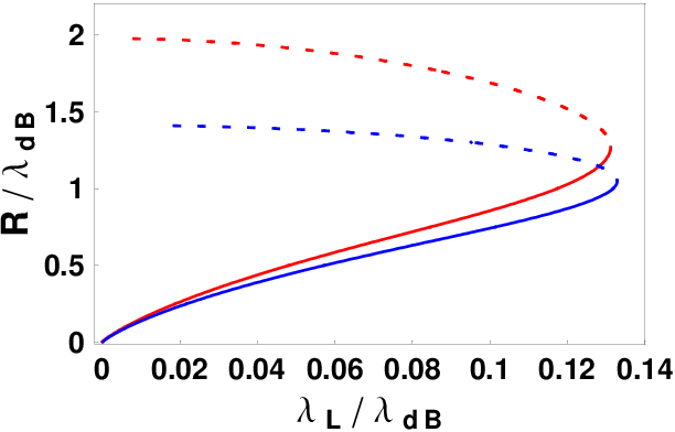
The distinguished feature is the existence of critical point for beyond which there will be no self-consistent solution: this occurs at roughly the same value for both displayed curves and we obtain the following condition for the existence of flux tube
| (62) |
Physically the above result is very appealing: it demonstrates the mechanism of how a flux tube which exists in the medium at low is eventually gone as the medium is heated up; on the other hand, for a medium with given it sets up a lower bound of monopole density that is required to support the existence of flux tube.
Another feature is that for each given smaller than the critical value, there are actually two solutions, one with small (typically smaller than 1, see solid curves) and the other with large (typically greater than 1, see dashed curves). This is understandable according to the complicated wiggle structure of . The solution with smaller radius is the stable one: it is much thinner and thus has stronger electric field (), which reflects monopoles more sharply near the boundary. The other solution with larger is unstable and should be discarded.
B Relativistic Gas
In relativistic gas the important scale is set by temperature, so let’s introduce the following dimensionless variables:
| (63) |
The fugacity , now in range , is related to density by
| (65) | |||||
with the number the degeneracy due to internal degrees of freedom. serves as normalization constant to momentum distribution (after scaling momenta by ).
The distribution over is given by
| (66) |
with . Similarly combining the above with eq.(22)(55) one obtains the relativistic version of the self-consistent equation
| (67) |
with given by the following integral
| (69) | |||||
We can further rewrite the self-consistent equation as
| (70) |
with the newly introduced relativistic parameters and .
For given sets of parameters (or equivalently ) one can easily find the flux tube size from the above equations by direct numerics. The situation is quite similar to the non-relativistic gas which we skip further discussion.
C Optimally Correlated Ensemble
Finally let’s discuss ensemble beyond an ideal gas. Clearly with significant interparticle correlations the ensemble may even not be easily describable by any distribution, however a typical momentum can still be invoked. A special situation which we call optimally correlated ensemble is that monopoles from such ensemble are largely carrying momenta within very narrow region around . On the contrary if the ensemble particles’ momenta are very diffusive in momentum space, it can hardly support flux tube.
In the optimally correlated ensemble, we approximate eq.(55) as (assuming NR formulae)
| (71) |
and the self-consistent equation is then given by
| (72) |
We limit the value of within beyond which there won’t be flux tube solution, as discussed in Section.IV C.
VI Disappearance of Flux Tubes in Quark-Gluon Plasma
Results from previous sections are general in nature and applicable to a variety of plasma physics problems. The present section, on the other hand, is dedicated to our main application, the physics of sQGP. From now on we switch to natural units and systematically put .
The existence of string/flux tubes in the QCD confined phase
is rather thoroughly investigated on lattice, via
measurements of static heavy quark potentials. Static free energy
potentials as a function of are only studied for
but for number of quark flavors as well as
physical QCD, see [32]. Those can be used to
extract the entropy and potential energy separately: the peaks of
these quantities (see e.g. Fig.2 of [33])
happen to be exactly at and then decrease toward larger
. The presence of the quasi-linear part of the energy and
entropy at intermediate leads to a conclusion that flux tubes
still exist at . Fig.8 from
[33] shows how both the internal energy and
entropy look like at . Unlike in the free energy (open
squares in the upper plot, in which cancellation takes place), the
internal energy (closed circles) still show at intermediate
a part linearly dependent on , while at
it very quickly disappears.

Why are flux tubes disappearing at large ? It can in principle be due to two different changes in QGP happening as T grows above , to be called (i) electric screening and (ii) magnetic penetration. The simplest mechanism (i) is that as grows beyond , the density of electrically charged quasiparticles -- gluons and quarks -- is growing and eventually it becomes large enough to screen heavy quarks. The reason for this density growth is the decrease in effective masses of electric excitations, which are lattice observables by themselves1414 14 See a related discussion of various color-electric objects’ effective masses in [34]. There we showed the masses are still rather large and their densities rather small at 1-1.5, limiting the screening.. At very large , in weak (electric) coupling domain, the screening of the potential is expected to be described by the Debye theory. However Debye theory does not describe entropy and internal energy associated with static quarks at , even at large distances, as can be seen e.g. from calculations of Antonov et al [35].
Another effect (ii), discussed for the first time in this work, is the penetration of magnetically charged quasiparticles (MQPs) inside the flux tubes, which destroys them. Indeed, the key parameter increases with and reaches the critical value eq.(74) for whether flux tube can exist or not. This imposes the following condition
| (75) |
Changing from upward the monopoles gets heavier and their dimensionless magnetic density keeps decreasing: eventually this will violate the flux tube condition. We thus identify the equality in (75) with the temperature at which local dissolution of the flux tubes takes place.
Furthermore, at we expect [1]. An independent consideration fixes conditions for monopole Bose condensation [29] which demands that around the monopole mass over temperature .
Combining these estimates with our critical condition for tube dissolution we obtain the density of magnetic quasiparticles at to be
| (76) |
which is within in absolute units.
Can the density of magnetic objects really be of that magnitude (which superficially looks rather high)? This estimated density includes in principle contributions from all types of magnetically charged objects in sQGP, i.e. not only pure adjoint monopoles but also self-dual dyons and also dyons containing quarks1515 15 We recall that monopoles have fermionic zero modes and states made of fermions travelling on top of a monopole have to be included as well. In supersymmetric theories those form spin-1/2 and even 1 magnetic objects, which are needed by supersymmetry to produced appropriate supermultiplets including the usual scalar monopoles..
Let us compare the numbers with whatever is mentioned in literature. We don’t know any studies of fermionic objects mentioned above.
Ilgenfritz et al [15] determined their dyon estimate by the caloron density, which is reliably calculated from the topological susceptibility. After multiplying by 3/2 their result for SU(2) we obtain density of self-dual dyons to be . Chernodub and Zakharov [36] mentioned the monopole density which is directly estimated from lattice configurations by following gauge-fixed monopoles along their trajectories. Their estimate is about . The sum of the two is consistent with the upper end of our estimate of what is needed for formation/dissolution of the flux tube.
Independent comparison can also be made with the vacuum () monopole density. Bali [22] has measured London penetration length by fitting lattice result with Abelian Higgs model. From that one can infer the monopole density to be as large as . Bornyakov et al [37] gave the vacuum monopole density to be about . All these results are well above our estimates for the density at “dissolution point”.
We believe all these numbers are consistent and suggest a coherent picture, of very dense monopole condensate in vacuum, tightly confining electric flux into very narrow tubes. When heated slightly above the monopole condensate changes into a non-condensed ensemble of monopoles, which is roughly twice less dense. Yet it is still capable of supporting flux tubes survived from vacuum, and only around the density of monopoles drops so low that there won’t be flux tube any more. At higher the electric sector becomes more and more dominant till eventually small number of heavy monopoles become embedded in the perturbative electric plasma.
VII Summary and outlook
In this paper we have studied stability of the electric flux tube in a monopole plasma. Quantum scattering of a single monopole on electric flux tube is analyzed in great details. Already classical analysis hints on the existence of a critical angular momentum dividing the scattered magnetic currents which support/dissolve the flux tube. This finding is quantitatively confirmed by quantum mechanic calculation, in which we have found exact scattering solutions to Schrodinger/Klein-Gordon equation in non-relativisitic/relativistic situations. These solutions allowed us to calculate the magnetic current produced, which is then averaged over the monopole ensemble and used in self-consistent determination of the flux tube size. The exact critical condition has been established, and applied to electric flux tube dissolution in sQGP system which interests us most. This leads to an estimate of total density of magnetic quasiparticles at , where lattice potentials indicate flux tube dissolution. These numbers are consistent with other studies using alternative ways to estimate magnetic density.
As mentioned in the introduction, this work is partly methodical in nature, ignoring electric quasiparticles which would lead to screening and termination of flux tubes. The next step we plan to do is obviously inclusion of both components and calculation of the static potentials. Hopefully, when one would consider an appropriate mixture of electric and magnetic quasiparticles, the lattice data on static potentials between electric and magnetic1616 16 Those are given by the expectation value of the so called ’t Hooft loop: we have not discussed them in this work. charges would be explained.
In principle, one should go beyond that and calculate field distributions around static charges as well. Lattice studies can be extended to measure directly electric/magnetic fields at : in fact the field profiles have been measured for flux tubes in vacuum before (see e.g. [22]).
Let us end with the following intriguing question. We focused above on electric flux in magnetic media, ignoring electric quasiparticles and possible dual phenomenon – a magnetic flux tube in an electric plasma. (We only mentioned their existence at low high density regime, in a color superconductor.) Now, may somewhere along the electric-magnetic equilibrium line there be conditions supporting stable flux tubes of types at the same time? It is known that confinement of both is impossible, but in a uncondensed plasma regime it may still be the case. A natural place to look for a QGP with intertwined electric and magnetic flux tubes is at less or of the order of , close to the place where three major phases – hadronic, color superconductor and QGP – meet. Although it is quite challenging task to get into this region using lattice gauge methods, the task is not hopeless.
Acknowledgments.
This work was supported in parts by the US-DOE grant DE-FG-88ER40388.
REFERENCES
- [1] J. Liao and E. Shuryak, Phys. Rev. C 75, 054907 (2007) [arXiv:hep-ph/0611131].
- [2] P. A. M. Dirac, Proc. Roy. Soc. Lond. A 133, 60 (1931).
- [3]
S. Mandelstam,
Phys. Rept. 23, 245 (1976).
G. ’t Hooft, “Topology Of The Gauge Condition And New Confinement Phases In Nonabelian Nucl. Phys. B 190, 455 (1981). - [4] N. Seiberg and E. Witten, Nucl. Phys. B 426, 19 (1994) [Erratum-ibid. B 430, 485 (1994)] [arXiv:hep-th/9407087].
- [5] A. G. Goldhaber and W. P. Trower, Am. J. Phys. 58, May 1990.
- [6] K. A. Milton, Rept. Prog. Phys.69, 1637 (2006) [arXiv: hep-ex/0602040].
- [7] J. A. Harvey, arXiv:hep-th/9603086.
- [8] E. J. Weinberg and P. Yi, Phys. Rept. 43, 65 (2007) [arXiv:hep-th/0609055].
- [9] M. Shifman and A. Yung, arXiv:hep-th/0703267.
- [10] Y. M. Shnir, “Magnetic Monopoles”, Berlin, Germany: Springer (2005).
- [11] E.V.Shuryak, Prog. Part. Nucl. Phys. 53, 273 (2004) [ hep-ph/0312227].
- [12] M. Gyulassy and L. McLerran, Nucl. Phys. A 750, 30 (2005). E. V. Shuryak,Prog.Part.Nucl.Phys.53, 273 (2004) [hep-ph/0312227]; Nucl. Phys. A 750, 64 (2005).
- [13] E. V. Shuryak, arXiv:hep-ph/0608177.
- [14] E. Shuryak, arXiv:hep-ph/0703208.
- [15] P. Gerhold, E. M. Ilgenfritz and M. Muller-Preussker, Nucl. Phys. B 760, 1 (2007) [arXiv:hep-ph/0607315].
- [16] D. Diakonov and V. Petrov, arXiv:0704.3181 [hep-th].
- [17] Y. Koma, M. Koma, E. M. Ilgenfritz, T. Suzuki and M. I. Polikarpov, Phys. Rev. D 68, 094018 (2003) [arXiv:hep-lat/0302006]. H. Shiba and T. Suzuki, Phys. Lett. B 351, 519 (1995) [arXiv:hep-lat/9408004].
- [18] A.A. Abrikosov, Sov. Phys. JETP 32, 1442 (1957).
- [19] H.B. Nielsen and P. Olesen, Nucl. Phys. B 61, 45 (1973).
- [20] M. Baker, J. S. Ball and F. Zachariasen, Phys. Rept. 209, 73 (1991).
- [21] G. Ripka, arXiv:hep-ph/0310102.
- [22] G. S. Bali, Quark confinement and the hadron spectrum III 17-36, Newport News 1998 [arXiv:hep-ph/9809351].
- [23] A. M. Polyakov, Phys. Lett. B 72, 477 (1978).
- [24] B. Bringoltz and M. Teper, PoS LAT2005, 175 (2006) [arXiv:hep-lat/0509186].
- [25] J. Liao and E. V. Shuryak, Nucl. Phys. A 775, 224 (2006) [arXiv:hep-ph/0508035].
- [26] G. ¡¯t Hooft, Nucl. Phys. B79, 276 (1974); A. M. Polyakov, JETP Lett. 20, 194 (1974) [Pisma Zh. Eksp. Teor. Fiz. 20, 430 (1974)].
- [27] E.B. Bogomol¡¯nyi, Sov. J. Nucl. Phys. 24, 449 (1976); M.K. Prasad and C.M. Sommerfield, Phys. Rev. Lett. 35, 760 (1975).
- [28] N.S. Manton, Nucl. Phys. B126, 525 (1977).
- [29] M. Cristoforetti and E. Shuryak, in preparation.
- [30] C. Ratti and E. Shuryak, in preparation.
- [31] C. P. Korthals Altes, arXiv:hep-ph/0607154; C. P. Korthals Altes and H. B. Meyer, arXiv:hep-ph/0509018.
- [32] O. Kaczmarek and F. Zantow, arXiv:hep-lat/0506019.
- [33] O. Kaczmarek and F. Zantow, PoS LAT2005, 192 (2006) [arXiv:hep-lat/0510094].
- [34] J. Liao and E. V. Shuryak, Phys. Rev. D 73, 014509 (2006) [arXiv:hep-ph/0510110].
- [35] D. Antonov, S. Domdey and H. J. Pirner, Nucl. Phys. A 789, 357 (2007) [arXiv:hep-ph/0612256].
- [36] M. N. Chernodub and V. I. Zakharov, Phys. Rev. Lett. 98, 082002 (2007) [arXiv:hep-ph/0611228].
- [37] V. G. Bornyakov, E. M. Ilgenfritz and M. Mueller-Preussker, Phys. Rev. D 72, 054511 (2005) [arXiv:hep-lat/0507021].