跳到论文正文
W Papers独立论文阅读器 arXiv:0706.4103 论文正文 计算阅读时间 · 0%
引用这篇论文根据当前论文元数据生成,正式投稿前建议核对。


License: arXiv.org perpetual non-exclusive license
arXiv:0706.4103v2 [math.AP] 09 Jun 2010

Practical Error Estimates for Reynolds’ Lubrication Approximation and its Higher Order CorrectionsThanks:  This work was supported in part by the Director, Office of Science, Advanced Scientific Computing Research, U.S. Department of Energy contract DE-AC02-05CH11231.

Jon Wilkening Thanks: Department of Mathematics and Lawrence Berkeley National Laboratory, University of California, Berkeley, CA 94720 (wilken@math.berkeley.edu).
Abstract

Reynolds’ lubrication approximation is used extensively to study flows between moving machine parts, in narrow channels, and in thin films. The solution of Reynolds’ equation may be thought of as the zeroth order term in an expansion of the solution of the Stokes equations in powers of the aspect ratio ε\varepsilon of the domain. In this paper, we show how to compute the terms in this expansion to arbitrary order on a two-dimensional, xx-periodic domain and derive rigorous, a priori error bounds for the difference between the exact solution and the truncated expansion solution. Unlike previous studies of this sort, the constants in our error bounds either are independent of the function h⁡(x)h(x) describing the geometry or depend on hh and its derivatives in an explicit, intuitive way. Specifically, if the expansion is truncated at order 2​k2k, the error is O⁡(ε2​k+2)O(\varepsilon^{2k+2}), and hh enters into the error bound only through its first and third inverse moments ∫01h​(x)−m​𝑑x\int_{0}^{1}h(x)^{-m}\,dx, m=1,3m=1,3, and via the max norms ‖1ℓ!​hℓ−1​∂xℓh‖∞\|\frac{1}{\ell!}h^{\ell-1}\partial_{x}^{\ell}h\|_{\infty}, 1≤ℓ≤2​k+21\leq\ell\leq 2k+2. We validate our estimates by comparing with finite element solutions and present numerical evidence that suggests that even when hh is real analytic and periodic, the expansion solution forms an asymptotic series rather than a convergent series.

keywords
incompressible flow, lubrication theory, asymptotic expansion, Stokes equations, thin domain, a priori error estimates
AMS
76D08, 35C20, 41A80
{DOI}

10.1137/070695447

1 Introduction

Reynolds’ lubrication equation [22, 20, 16, 12] is used extensively in engineering applications to study flows between moving machine parts, e.g., in journal bearings or computer disk drives. It is also used in microfluid and bio-fluid mechanics to model creeping flows through narrow channels and in thin films. Although there is a vast literature (including several textbooks) on viscous flows in thin geometries, the equations are normally derived either directly from physical arguments [16] or using formal asymptotic arguments [12]. This is acceptable in most circumstances as the original equations (Stokes or Navier–Stokes) have also been derived from physical considerations, and by now the lubrication equations have been used frequently enough that one can draw on experience and intuition to determine whether they will work well for a given problem.

On the other hand, as soon as the geometry of interest develops (or approaches) a singularity, or if we wish to compute several terms in the asymptotic expansion of the solution in powers of the aspect ratio ε\varepsilon, we rapidly leave the space of problems for which we can use experience as a guide; thus, it would be helpful to have a rigorous proof of convergence to serve as a guide to identify the features of the geometry that could potentially invalidate the approximation. For example, in [25], Wilkening and Hosoi used lubrication theory to study the optimal wave shapes that an animal such as a gastropod should use as it propagates ripples along its muscular foot to crawl over a thin layer of viscous fluid. In certain limits of this constrained optimization problem, the optimal wave shape develops a kink or cusp in the vicinity of the region closest to the substrate, and there is a competing mechanism controlling the size of the modeling error (singularity formation versus nearness to the substrate). We found that shape optimization within (zeroth order) lubrication theory drives the geometry out of the realm of applicability of the lubrication model; however, by computing higher order corrections and monitoring the errors (using the results of this paper), we learned that cusp-like singularities are appropriately penalized by the full Stokes equations, yielding nonsingular optimal solutions; see [25] for further details.

1.1 Previous work

In most of the following papers, the Stokes or Navier–Stokes equations are solved in a domain Ωε\Omega_{\varepsilon} bounded below by a flat substrate and above by a curved boundary y=ε​h​(x)y=\varepsilon h(x) in two dimensions, or z=ε​h​(x,y)z=\varepsilon h(x,y) in three dimensions, where ε\varepsilon is a small parameter and the function hh is fixed. These solutions are then compared to the solution of Reynolds’ equation (or to a truncated expansion solution of the Stokes or Navier–Stokes equations), and the error is shown to converge to zero in the limit as ε→0\varepsilon\rightarrow 0.

In 1983, Cimatti [8] used a stream function formulation to compare the solution of Reynolds’ equation to that of the Stokes equation in two dimensions. The key idea of the proof, which all subsequent studies (including this one) also use, is that the Poincaré–Friedrichs inequality holds uniformly as ε→0\varepsilon\rightarrow 0 for the rescaled biharmonic equation (where the domain Ω=Ωε=1\Omega=\Omega_{\varepsilon=1} is held fixed and the equations contain the small parameter). Cimatti assumes hh has four weak derivatives (whereas, we require only h∈C1,1h\in C^{1,1}) and shows that for any compact set K⊂ΩK\subset\Omega,

(1) ‖ε​u−u¯‖L2​(Ω)≤C​ε,max⁡(‖ε3​px−p¯x‖L2​(K),‖ε2​py‖L2​(K))≤C​ε1/2,\|\varepsilon u-\bar{u}\|_{L^{2}(\Omega)}\leq C\varepsilon,\qquad\max\left(\|\varepsilon^{3}p_{x}-\bar{p}_{x}\|_{L^{2}(K)},\|\varepsilon^{2}p_{y}\|_{L^{2}(K)}\right)\leq C\varepsilon^{1/2},

where uu is the xx-component of velocity, pp is the pressure, a bar denotes the solution of Reynolds’ equation, and CC is independent of ε\varepsilon but depends on hh in the first inequality and on hh and KK in the second. The scaling here in not standard: he imposes the boundary condition εu(x,0)=u¯(x,0)=const\varepsilon u(x,0)=\bar{u}(x,0)=\mathop{\operator@font const}\nolimits, which accounts for the extra factor of ε\varepsilon in each of the left-hand sides of (1). There are a few problems with Cimatti’s analysis, notably the dependence of CC on LL (the “arbitrary cutoff” used to make the unbounded domain bounded) and the fact that some of his arguments seem to require ε\varepsilon to be small in comparison to C−1C^{-1}; however, his basic approach is interesting and inspired much of the work that followed in this subject.

In 1986, Bayada and Chambat [3] generalized Cimatti’s work to three dimensions. They analyze the Stokes equations directly rather than using a stream function formulation, assume less regularity of hh (apparently only h∈C1h\in C^{1}), and state their results in terms of limits (i.e., the quantities uiεu^{\varepsilon}_{i}, ε​∂xuiε\varepsilon\partial_{x}u^{\varepsilon}_{i}, ∂yuiε\partial_{y}u^{\varepsilon}_{i}, and pεp^{\varepsilon} in the solution of the Stokes equations converge in L2L^{2} to the corresponding quantities in the solution of Reynolds equations as ε→0\varepsilon\rightarrow 0); hence, they do not give rates of convergence. In a later paper [4], they also studied the asymptotics of the solution at a junction between a three-dimensional Stokes flow and a thin film flow.

In 1990, Nazarov [18] generalized previous work to the case of the Navier–Stokes equations and also showed how to treat higher order corrections in an asymptotic expansion in the small parameter ε\varepsilon. He proved that if h⁡(x,y)h(x,y) is smooth, then there is a constant CC depending on hh, NN, and the boundary conditions such that

(2) ‖𝐮−𝐮N‖H1+‖p−ε−1​pN‖L2≤C​εN−1/2,\left\|\mathbf{u}-\mathbf{u}^{N}\right\|_{H^{1}}+\left\|p-\varepsilon^{-1}p^{N}\right\|_{L^{2}}\leq C\varepsilon^{N-1/2},

where (𝐮,p)(\mathbf{u},p) is the solution of the Navier–Stokes equations, 𝐮N\mathbf{u}^{N} and pNp^{N} are the terms of the asymptotic expansion truncated at the NNth order (including a boundary layer expansion near the lateral edges of the thin domain), and the norms are taken on the thin domain Ωε\Omega_{\varepsilon} (rather than the rescaled domain Ω\Omega). As a corollary, if the expansion is computed with “superfluous” terms that are afterwards treated as remainders, he obtains the optimal estimate

(3) ‖𝐮−𝐮N‖L2+ε1/2‖(π1/2ε∇)(𝐮−𝐮N)‖L2+‖p−ε−1pN‖L2≤CεN+1.\left\|\mathbf{u}-\mathbf{u}^{N}\right\|_{L^{2}}+\varepsilon^{1/2}\left\|\left(\pi_{1/2}^{\varepsilon}\nabla\right)\left(\mathbf{u}-\mathbf{u}^{N}\right)\right\|_{L^{2}}+\left\|p-\varepsilon^{-1}p^{N}\right\|_{L^{2}}\leq C\varepsilon^{N+1}.

Nazarov’s paper is concise to the point of being impenetrable at times. We interpret π1/2ε∇=(∂x,∂y,ε1/2∂z)\pi_{1/2}^{\varepsilon}\nabla=(\partial_{x},\partial_{y},\varepsilon^{1/2}\partial_{z}), but this symbol was not defined and may actually be a variable coefficient operator that incorporates the boundary conditions in its definition. We are also unsure of the definition of pp and pNp^{N}, as we would have expected p−ε−2​pNp-\varepsilon^{-2}p^{N} to appear together.

In a later paper [19], Nazarov studies the asymptotics of the solution of the Stokes equations in a domain in which two smooth surfaces meet at a point. This problem is also studied in a recent paper of Ciuperca, Hafidi, and Jai in [9]. This singular limit is interesting in that deriving even the first correction to the zeroth order approximation in the asymptotic expansion remains an open problem.

Assemien, Bayada, and Chambat [2] have studied the important question of the effect of inertia on the asymptotic behavior of a thin film flow, which can in many cases be significant, requiring that the Navier–Stokes equations be used in place of the Stokes equations as the underlying model for the asymptotic expansion. We also mention that there is a large body of literature on the long-time behavior of solutions of the Navier–Stokes equations on thin domains; see, e.g., [21, 17].

In 2000, Duvnjak and Marus̆ić-Paloka [11] showed how to rigorously analyze the lubrication approximation of the Navier–Stokes equations for a slipper bearing in a circular geometry. The focus of their paper is on formulating the problem in cylindrical coordinates and showing how to adapt the zeroth order case of Nazarov’s proof to handle the change of variables. Elrod’s pioneering 1960 paper [12] is also concerned with the (formal) relationship between the Navier–Stokes equations and Reynolds’ equation for this geometry.

1.2 Motivation and summary

None of the studies described above shows how the constant CC bounding the error depends on the function h⁡(x)h(x) describing the geometry. This is because most theorems of analysis give constants that depend on the domain Ω\Omega, which is usually fixed. But in our case, the data h⁡(x)h(x) of the problem actually specifies the domain; therefore, to obtain bounds that are independent of hh, one must avoid or modify standard arguments for flattening the boundary, etc., so as not to lose track of h⁡(x)h(x) in the analysis. Moreover, arguments based on the closed graph theorem or Rellich’s compactness theorem must be avoided entirely, as these also depend on the geometry. This forces us to look for new ways to analyze old problems using tools that furnish explicit constants.

In this paper, we consider only the two-dimensional, periodic Stokes equations with a specific choice of boundary conditions, but we derive error estimates that depend on hh in an explicit, intuitive way. Our main result is summarized in Theorem 18, which may be stated as follows: Let T=[0,1]pT=[0,1]_{p} be the periodic unit interval. If k≥0k\geq 0, h∈C2​k+1,1​(T)h\in C^{2k+1,1}(T), 0<h0≤h⁡(x)≤10<h_{0}\leq h(x)\leq 1 for x∈Tx\in T, and ε≤r0/3\varepsilon\leq r_{0}/3 (defined below), then the error in truncating the expansion of the stream function, velocity, vorticity, and pressure (in appropriate ε\varepsilon-weighted Sobolev norms) at order 2​k2k (keeping in mind that only even powers of ε\varepsilon appear in these expansions) is bounded by

(4) I1​(|V0|+|V1|)​[1+θk​εrk​I3I1]​(ερk​rk)2​k+2,\sqrt{I_{1}}\left(|V_{0}|+|V_{1}|\right)\left[1+\theta_{k}\frac{\varepsilon}{r_{k}}\sqrt{\frac{I_{3}}{I_{1}}}\right]\left(\frac{\varepsilon}{\rho_{k}r_{k}}\right)^{2k+2},

where V0V_{0} and V1V_{1} are prescribed tangential velocities on the lower and upper boundaries of the domain

(5) rk=(max1≤ℓ≤2​k+2⁡{‖1ℓ!​hℓ−1​∂xℓh‖∞1/ℓ})−1,Im=∫01h​(x)−m​𝑑xr_{k}=\left(\max_{1\leq\ell\leq 2k+2}\left\{\left\|\frac{1}{\ell!}h^{\ell-1}\partial_{x}^{\ell}h\right\|_{\infty}^{1/\ell}\right\}\right)^{-1},\qquad I_{m}=\int_{0}^{1}h(x)^{-m}\,dx

and ρk\rho_{k}, θk\theta_{k} are constants independent of hh. The bound on pressure has another term involving h0h_{0}; see (169) below.

The constants in (4) have been divided into two types: those that are (1) given in the problem statement or easily computable from hh; or (2) difficult to compute but universal (independent of hh). We show how to compute the constants in the latter category (ρk\rho_{k} and θk\theta_{k}) in section 4; see Table 4. The constants in the former category (rkr_{k} and ImI_{m}) help us understand the competing mechanism of singularity formation versus proximity to the substrate: the curvature and higher derivatives are allowed to diverge as long as the gap size simultaneously approaches zero in such a way that the homogeneous products 1ℓ!​hℓ−1​∂xℓh\frac{1}{\ell!}h^{\ell-1}\partial_{x}^{\ell}h remain uniformly bounded. Although the factors I1\sqrt{I_{1}} and I3/I1\sqrt{I_{3}/I_{1}} in (4) also diverge in this limit, the norm of the exact solution diverges at a similar rate — so the relative error in the expansion solution truncated at order 2​k2k is O⁡(ε2​k+2)O(\varepsilon^{2k+2}), with ρk​rk\rho_{k}r_{k} serving as an effective radius of convergence.

The framework we have chosen for this paper is intended to be general enough to cover many interesting applications (such as a crawling gastropod [25] or an “unwrapped” slipper bearing) but simple enough to obtain explicit detailed estimates that reveal the dependence of the error on the geometry h⁡(x)h(x). We also wanted to determine whether there might exist geometries for which the asymptotic expansion yields a convergent series. Although we do not have a rigorous proof, the answer appears to be negative even for the simplest case of a real analytic function such as h⁡(x)=35+25​sin⁡2​π​xh(x)=\frac{3}{5}+\frac{2}{5}\sin 2\pi x, for which the rkr_{k} in (5) are bounded away from zero. It is hoped that this work will serve as a useful first step toward obtaining similar error estimates for three-dimensional problems that include more general boundary conditions, incorporate end effects near the lateral edges of the domain (which we avoid by studying the periodic case), and include the effect of inertia or viscoelasticity.

1.3 Outline

In section 2, we derive Reynolds’ lubrication approximation in its primitive and stream function formulations. In section 3, we show how to compute successive terms in an asymptotic expansion of the stream function. In section 3.2, we prove a structure theorem describing the dependence of these terms on h⁡(x)h(x) and its derivatives.

In section 4, we formulate the problem weakly and analyze the truncation error equation using weighted Sobolev spaces and a uniform Poincaré–Friedrichs argument. The first challenge is to find the right weighted norms on the lower and upper boundaries (equivalent to H1/2​(Γ0)H^{1/2}(\Gamma_{0}) and H1/2​(Γ1)H^{1/2}(\Gamma_{1}) for fixed ε\varepsilon) to yield manageable error estimates in terms of hh when we change variables to straighten out the boundaries. In section 4.4, we reduce the problem of bounding the truncation errors to that of bounding the second and fourth derivatives of the two highest order terms retained in the asymptotic expansion, namely, ‖ψx​x(2​k)‖0\|\psi_{xx}^{(2k)}\|_{0} and ‖h2​ψx​x​x​x(2​k−2)‖0\|h^{2}\psi_{xxxx}^{(2k-2)}\|_{0}. We then use the structure theorem of section 3.2 to compute these norms in order to obtain the constants ρk\rho_{k} and θk\theta_{k} in (4) for 0≤k≤250\leq k\leq 25. In section 4.5, we show how to compute the error in velocity, vorticity, and pressure from that of the stream function. This requires that we determine how the Babus̆ka–Brezzi inf-sup constant β\beta depends on h⁡(x)h(x); see [24].

In section 5, we validate our results by comparing to “exact” solutions (computed using finite elements) for a geometry typical of engineering applications. The result of this comparison is that the effective radius of convergence rk​ρkr_{k}\rho_{k} is within a factor of 3 of optimal for k=5k=5, k=10k=10, and perhaps all k≥5k\geq 5. These calculations also suggest that even when h⁡(x)h(x) is real analytic, the expansion solution is an asymptotic series rather than a convergent series. This is because the constants ρk\rho_{k} converge to zero as k→∞k\rightarrow\infty. Fortunately, ρk\rho_{k} initially increases and does not become smaller than ρ0=0.197\rho_{0}=0.197 until 2​k=262k=26, which is already outside of the practical range of kk. Finally, in Appendix A, we present our numerical algorithm for computing the expansion solutions, which can be performed symbolically using a computer algebra system such as Mathematica or in floating point arithmetic, e.g., in C+⁣+C^{++}.

2 Reynolds’ approximation

Consider the Stokes equations on a periodic domain of width W¯\bar{W} bounded below by a flat wall moving with constant speed V¯0\bar{V}_{0} and above by an inextensible sheet moving with constant speed V¯1\bar{V}_{1} along a fixed curve Γ1,ε={(x¯,h¯​(x¯)):0≤x¯≤W¯}\Gamma_{1,\varepsilon}=\{(\bar{x},\bar{h}(\bar{x})):0\leq\bar{x}\leq\bar{W}\}; see Figure 1. A bar is used to distinguish a physical variable from its dimensionless counterpart. We nondimensionalize the variables by choosing a characteristic speed U¯\bar{U} and height H¯\bar{H} for the problem, and set x¯=W¯​x\bar{x}=\bar{W}x, y¯=H¯​y\bar{y}=\bar{H}y, h¯​(x¯)=H¯​h​(x)\bar{h}(\bar{x})=\bar{H}h(x), V¯i=U¯​Vi\bar{V}_{i}=\bar{U}V_{i}, (u¯,v¯)=𝐮¯=(U¯​u,U¯​H¯W¯​v)(\bar{u},\bar{v})=\bar{\mathbf{u}}=(\bar{U}u,\bar{U}\frac{\bar{H}}{\bar{W}}v),

and p¯=μ¯​U¯​W¯H¯2​p\bar{p}=\bar{\mu}\frac{\bar{U}\bar{W}}{\bar{H}^{2}}p. The stream function ψ\psi, flux QQ, and vorticity ω\omega introduced below satisfy

ψ¯=U¯​H¯​ψ\bar{\psi}=\bar{U}\bar{H}\psi, Q¯=U¯​H¯​Q\bar{Q}=\bar{U}\bar{H}Q, and ω¯=U¯H¯​ω\bar{\omega}=\frac{\bar{U}}{\bar{H}}\omega.

Refer to caption   Refer to caption

Fig. 1: Geometry commonly encountered in lubrication-type problems. Left: Physical coordinate system. Right: Dimensionless coordinate system (Δε=ε2∂x2+∂y2\Delta_{\varepsilon}=\varepsilon^{2}\partial_{x}^{2}+\partial_{y}^{2}).

We have in mind a situation where the aspect ratio ε=H¯/W¯\varepsilon=\bar{H}/\bar{W} of the physical domain is small. By scaling the xx- and yy-axes differently, we map the problem onto a nicer geometry, which introduces terms in the equations that vanish in the singular limit ε→0\varepsilon\rightarrow 0. Specifically, we wish to find xx-periodic functions u,v,pu,v,p defined on the rescaled domain

(6) Ω={(x,y): 0≤x≤1,  0<y<h(x)}\Omega=\{(x,y)\;:\;0\leq x\leq 1,\;\;0<y<h(x)\}

such that

(7) px=ε2ux​x+uy​y,py=ε4vx​x+ε2vy​y,vy=−ux(in Ω)p_{x}=\varepsilon^{2}u_{xx}+u_{yy},\qquad p_{y}=\varepsilon^{4}v_{xx}+\varepsilon^{2}v_{yy},\qquad v_{y}=-u_{x}\qquad(\text{in }\Omega)

subject to periodic boundary conditions on the left and right sides of Ω\Omega and

(8) (u,v)|=Γ0(g0,0),(u,v)|Γ1=(g1,hxg1)(u,v)\left|{}_{\Gamma_{0}}=(g_{0},0),\qquad(u,v)\right|_{\Gamma_{1}}=(g_{1},h_{x}g_{1})

on the bottom and top boundaries. Here

(9) g0(x)=V0,g1(x)=V1[1+ε2h′(x)2]−1/2,g_{0}(x)=V_{0},\qquad g_{1}(x)=V_{1}\left[1+\varepsilon^{2}h^{\prime}(x)^{2}\right]^{-1/2},

i.e., g1​(x)=V1​cos⁡θ⁡(x)g_{1}(x)=V_{1}\cos\theta(x), where  θ=arctan⁡(ε​hx)\theta=\arctan(\varepsilon h_{x})  is the angle of the curve h¯​(x¯)\bar{h}(\bar{x}) relative to the horizontal. Reynolds’ lubrication approximation is obtained by setting ε=0\varepsilon=0 in the equations and solving

(10) px=uy​y,py=0,vy=−ux,𝐮|=Γ0(V0;0),𝐮|Γ1=(1;hx)V1.p_{x}=u_{yy},\quad\;\;p_{y}=0,\quad\;\;v_{y}=-u_{x},\quad\;\;\mathbf{u}\left|{}_{\Gamma_{0}}=(V_{0};0),\quad\;\;\mathbf{u}\right|_{\Gamma_{1}}=(1;h_{x})V_{1}.

If we write (7) in the form L⁡(𝐮,p)=(0,0,0)L(\mathbf{u};p)=(0;0;0), where L=L(0)+ε2​L(2)+ε4​L(4)L=L^{(0)}+\varepsilon^{2}L^{(2)}+\varepsilon^{4}L^{(4)} is given by

(11) L=(−∂y20∂x00∂y∂x∂y0)+ε2​(−∂x2000−∂y20000)+ε4​(0000−∂x20000),L=\begin{pmatrix}-\partial_{y}^{2}&0&\partial_{x}\\ \phantom{-}0&0&\partial_{y}\\ \phantom{-}\partial_{x}&\partial_{y}&0\end{pmatrix}+\varepsilon^{2}\begin{pmatrix}-\partial_{x}^{2}&\phantom{-}0&0\\ \phantom{-}0&-\partial_{y}^{2}&0\\ \phantom{-}0&\phantom{-}0&0\end{pmatrix}+\varepsilon^{4}\begin{pmatrix}0&\phantom{-}0&0\\ 0&-\partial_{x}^{2}&0\\ 0&\phantom{-}0&0\end{pmatrix},

then (10) is just the zeroth order system L(0)​(𝐮,p)=(0,0,0)L^{(0)}(\mathbf{u};p)=(0;0;0) with zeroth order boundary conditions (expanding g0g_{0} and g1g_{1} in (8) in powers of ε\varepsilon). The equation for vv decouples from the others, and we find that pp is independent of yy and

(12) u⁡(x,y)=(y22−h⁡(x)​y2)​px​(x)+(1−yh⁡(x))​V0+yh⁡(x)​V1.u(x,y)=\left(\frac{y^{2}}{2}-\frac{h(x)y}{2}\right)p_{x}(x)+\left(1-\frac{y}{h(x)}\right)V_{0}+\frac{y}{h(x)}V_{1}.

Integrating from 00 to hh and solving for pxp_{x}, we obtain

(13) px=6h2​(V0+V1)−12h3​Q,p_{x}=\frac{6}{h^{2}}(V_{0}+V_{1})-\frac{12}{h^{3}}Q,

where Q=∫0hu⁡(x,y)​𝑑yQ=\int_{0}^{h}u(x,y)\,dy is the volume flux through any cross section of the fluid. (QQ is constant since ∇⋅𝐮=0\nabla\cdot\mathbf{u}=0 and 𝐮\mathbf{u} is tangent to Γ0\Gamma_{0} and Γ1\Gamma_{1}). Since pp is periodic, ∫px​𝑑x=0\int p_{x}\,dx=0, and we find that

(14) Q=V0+V12​I2I3(Im=∫01h​(x)−m​𝑑x).Q=\frac{V_{0}+V_{1}}{2}\frac{I_{2}}{I_{3}}\qquad\qquad\left(I_{m}=\int_{0}^{1}h(x)^{-m}\,dx\right).

Substituting (14) and (13) into (12) and using vy=−uxv_{y}=-u_{x}, v⁡(x,0)=0v(x,0)=0, we obtain the solution

px\displaystyle p_{x} =6​(V0+V1)h2​(1−I2I3​h),\displaystyle=\frac{6(V_{0}+V_{1})}{h^{2}}\left(1-\frac{I_{2}}{I_{3}h}\right),
(15) u\displaystyle u =(V0+V1)​(3​I2I3​h−3)​(yh−y2h2)+(1−yh)​V0+yh​V1,\displaystyle=(V_{0}+V_{1})\left(3\frac{I_{2}}{I_{3}h}-3\right)\left(\frac{y}{h}-\frac{y^{2}}{h^{2}}\right)+\left(1-\frac{y}{h}\right)V_{0}+\frac{y}{h}V_{1},
v\displaystyle v =(V0+V1)​(3​I2I3​h−2)​(y2h2−y3h3)​hx+V1​y2h2​hx.\displaystyle=(V_{0}+V_{1})\left(3\frac{I_{2}}{I_{3}h}-2\right)\left(\frac{y^{2}}{h^{2}}-\frac{y^{3}}{h^{3}}\right)h_{x}+V_{1}\frac{y^{2}}{h^{2}}h_{x}.

The vertical component vv of the velocity field is customarily omitted from zeroth order lubrication theory as v¯=ε​U¯​v\bar{v}=\varepsilon\bar{U}v is O⁡(ε)O(\varepsilon) on the thin geometry Ωε\Omega_{\varepsilon} of Figure 1.

We may also derive (15) using a stream function formulation of the problem. Our procedure for computing higher order corrections to the lubrication approximation and our method for estimating the error of these expansion solutions are both done in the stream function formulation. Let us define

(16) Δε=ε2∂x2+∂y2,𝐮ε=(uε2​v).\Delta_{\varepsilon}=\varepsilon^{2}\partial_{x}^{2}+\partial_{y}^{2},\qquad\qquad\mathbf{u}_{\varepsilon}=\begin{pmatrix}u\\ \varepsilon^{2}v\end{pmatrix}.

In our error estimates below, we will need to consider the inhomogeneous problem L⁡(𝐮,p)=(F1,F2,0)L(\mathbf{u};p)=(F_{1};F_{2};0) with boundary conditions (8), i.e.,

(17) −Δε​𝐮ε+∇p=𝐅,∇⋅𝐮=0,𝐮|=Γ0(g0;0),𝐮|Γ1=(g1;hxg1).\begin{aligned} -\Delta_{\varepsilon}\mathbf{u}_{\varepsilon}+\nabla p&=\mathbf{F},\\ \nabla\cdot\mathbf{u}&=0,\end{aligned}\qquad\mathbf{u}\left|{}_{\Gamma_{0}}=(g_{0};0),\qquad\mathbf{u}\right|_{\Gamma_{1}}=(g_{1};h_{x}g_{1}).

Since 𝐮\mathbf{u} is incompressible, there is a stream function ψ\psi such that

(18) 𝐮=∇×ψ=(ψy,−ψx),∇×𝐮ε=ε2​vx−uy=−Δε​ψ.\mathbf{u}=\nabla\times\psi=(\psi_{y},-\psi_{x}),\qquad\nabla\times\mathbf{u}_{\varepsilon}=\varepsilon^{2}v_{x}-u_{y}=-\Delta_{\varepsilon}\psi.

It follows from (17) that ψ\psi satisfies the rescaled biharmonic equation

(19) Δε2​ψ=ψy​y​y​y+2​ε2​ψx​x​y​y+ε4​ψx​x​x​x=∇×𝐅,\Delta_{\varepsilon}^{2}\psi=\psi_{yyyy}+2\varepsilon^{2}\psi_{xxyy}+\varepsilon^{4}\psi_{xxxx}=\nabla\times\mathbf{F},

with periodic boundary conditions in the xx-direction and

(20) {ψ=0ψy=g0}​ on ​Γ0,{ψ=Qψy​(x,h​(x))=g1}​ on ​Γ1,\left\{\begin{aligned} \psi&=0\\ \psi_{y}&=g_{0}\end{aligned}\right\}\text{ on }\Gamma_{0},\qquad\left\{\begin{aligned} \psi&=Q\\ \psi_{y}(x,h(x))&=g_{1}\end{aligned}\right\}\text{ on }\Gamma_{1},

where Q=∫0h⁡(0)u⁡(0,y)​𝑑yQ=\int_{0}^{h(0)}u(0,y)\,dy. Since pp is periodic, ∫01px​(x,0)​𝑑x=0\int_{0}^{1}p_{x}(x,0)\,dx=0, i.e.,

(21) ∫01ψy​y​y​(x,0)+F1​(x,0)​𝑑x=0.\int_{0}^{1}\psi_{yyy}(x,0)+F_{1}(x,0)\,dx=0.

Conversely, suppose we are able to find a flux QQ and a classical solution ψ\psi of (19) and (20) such that (21) holds. Then we define 𝐮=∇×ψ\mathbf{u}=\nabla\times\psi and note that (19) implies ∇×(Δε​𝐮ε+𝐅)≡0\nabla\times(\Delta_{\varepsilon}\mathbf{u}_{\varepsilon}+\mathbf{F})\equiv 0, i.e., the integral

(22) p(x,y)=∫γ(Δε𝐮ε+𝐅)⋅𝐭ds,(𝐭 = unit tangent vector along path γ joining (0,0) to (x,y))p(x,y)=\int_{\gamma}(\Delta_{\varepsilon}\mathbf{u}_{\varepsilon}+\mathbf{F})\cdot\mathbf{t}\,ds,\qquad\left(\parbox{144.54pt}{\begin{center}$\mathbf{t}$ $=$ unit tangent vector along path $\gamma$ joining $(0,0)$ to $(x,y)$\end{center}}\right)

is independent of the path γ\gamma. A canonical choice for γ\gamma is

(23) p⁡(x,y)=∫0x[ε2​ux​x+uy​y+F1]​(ξ,0)​𝑑ξ+∫0y[ε4​vx​x+ε2​vy​y+F2]​(x,η)​𝑑η.p(x,y)=\int_{0}^{x}\left[\varepsilon^{2}u_{xx}+u_{yy}+F_{1}\right](\xi,0)\,d\xi+\int_{0}^{y}\left[\varepsilon^{4}v_{xx}+\varepsilon^{2}v_{yy}+F_{2}\right](x,\eta)\,d\eta.

Condition (21) is equivalent to requiring p⁡(1,0)=p⁡(0,0)p(1,0)=p(0,0), from which it follows that p⁡(1,y)=p⁡(0,y)p(1,y)=p(0,y) for 0≤y≤h⁡(0)0\leq y\leq h(0), since the integrand of the second integral in (23) is periodic in xx. By construction, the variables 𝐮\mathbf{u}, pp satisfy (17), where the boundary condition on Γ1\Gamma_{1} follows from the fact that ψx+hx​ψy=0\psi_{x}+h_{x}\psi_{y}=0 there; hence, classical solutions of the rescaled biharmonic equation yield classical solutions of the rescaled Stokes equations and vice versa. Reynolds’ approximation (15) is recovered if 𝐅\mathbf{F} and ε\varepsilon are set to zero in (19)–(21) when solving for ψ\psi and QQ; see section 3.1.

3 Higher order corrections

In this section we show how to compute successive terms in the formal expansion of the solution of the rescaled biharmonic equation (19) in powers of ε=H¯/W¯\varepsilon=\bar{H}/\bar{W}. For this purpose, it is convenient to manipulate the equations assuming they are satisfied classically. Once we obtain formulas for the higher order approximations, we will show (in section 4) that they satisfy a weak formulation of the problem that makes it possible to obtain error estimates. See [15] for background on perturbation methods in partial differential equations.

3.1 A recursive algorithm

Matching like powers of ε\varepsilon in the expansion

(24) [∂y4+2ε2∂x2∂y2+ε4∂x4][ψ(0)+ε2ψ(2)+ε4ψ(4)+⋯]=0,\left[\partial_{y}^{4}+2\varepsilon^{2}\partial_{x}^{2}\partial_{y}^{2}+\varepsilon^{4}\partial_{x}^{4}\right]\left[\psi^{(0)}+\varepsilon^{2}\psi^{(2)}+\varepsilon^{4}\psi^{(4)}+\cdots\right]=0,

we obtain the recursion

ψy​y​y​y(0)\displaystyle\psi^{(0)}_{yyyy} =0,\displaystyle=0,
ψy​y​y​y(2)\displaystyle\psi^{(2)}_{yyyy} =−2​ψx​x​y​y(0),\displaystyle=-2\psi^{(0)}_{xxyy},
(25) ψy​y​y​y(2​k)\displaystyle\psi^{(2k)}_{yyyy} =−2​ψx​x​y​y(2​k−2)−ψx​x​x​x(2​k−4),\displaystyle=-2\psi^{(2k-2)}_{xxyy}-\psi^{(2k-4)}_{xxxx}, k=2,3,4,….\displaystyle k=2,3,4,\dotsc.
The boundary conditions (20) become
(26) B​ψ(2​k)\displaystyle B\psi^{(2k)} =(0,g0(2​k),Q(2​k),g1(2​k)),\displaystyle=\left(0,g_{0}^{(2k)},Q^{(2k)},g_{1}^{(2k)}\right), k=0,1,2,3,…,\displaystyle k=0,1,2,3,\dotsc,

where B​ψ=(ψ|Γ0,ψy|Γ0,ψ|Γ1,ψy|Γ1)B\psi=(\psi|_{\Gamma_{0}},\psi_{y}|_{\Gamma_{0}},\psi|_{\Gamma_{1}},\psi_{y}|_{\Gamma_{1}}) and g0​(x)g_{0}(x), g1​(x)g_{1}(x) were defined in (9):

(27) g0(2​k)​(x)={V0,k=0,0,k>0,g1(2​k)​(x)=V1​(−1/2k)​h′​(x)2​k.g_{0}^{(2k)}(x)=\begin{cases}V_{0},&k=0,\\ 0,&k>0,\end{cases}\qquad g_{1}^{(2k)}(x)=V_{1}{-1/2\choose k}h^{\prime}(x)^{2k}.

Condition (21) (with F1=0F_{1}=0) becomes

(28) ∫01ψy​y​y(2​k)(x,0)dx=0,k=0,1,2,….\int_{0}^{1}\psi^{(2k)}_{yyy}(x,0)\,dx=0,\qquad k=0,1,2,\dotsc.

If 𝐅\mathbf{F} were nonzero in (19) and depended on ε\varepsilon in such a way that ∇×𝐅\nabla\times\mathbf{F} had an expansion in even powers of ε\varepsilon, we could incorporate these terms into (25) and (28) as well; however, we will assume 𝐅=𝟎\mathbf{F}=\mathbf{0} except in section 4, where we consider the general case only to derive error estimates for the 𝐅=𝟎\mathbf{F}=\mathbf{0} case. Let us denote the right-hand side of (25) by f(2​k)​(x,y)f^{(2k)}(x,y) for k≥0k\geq 0. The terms ψ(2​k)\psi^{(2k)}, Q(2​k)Q^{(2k)} in (25) and (26) may be computed via

(29) (ψ(2​k),Q(2​k))=G(f(2​k),g0(2​k),g1(2​k)),k=0,1,2,…,\left(\psi^{(2k)},Q^{(2k)}\right)=G\left(f^{(2k)},\;g_{0}^{(2k)},\;g_{1}^{(2k)}\right),\qquad k=0,1,2,\dotsc,

where GG is defined by Algorithm 1 in Figure 2.

Algorithm 1.
(ψ,Q)=G⁡(f,g0,g1)(\psi,Q)=G(f,g_{0},g_{1}): ψ0=𝕍4​f\psi_{0}=\mathbb{V}^{4}f   (𝕍=Volterra operator: 𝕍f(x,y)=∫0yf(x,η)dη)\left(\mathbb{V}=\mbox{Volterra operator: }\displaystyle\mathbb{V}f(x,y)=\int_{0}^{y}f(x,\eta)\,d\eta\right) Q=12​I3​∫012​ψ0​(x,h⁡(x))h​(x)3+−ψ0,y​(x,h⁡(x))+g0+g1​(x)h​(x)2​𝑑x\displaystyle Q=\frac{1}{2I_{3}}\int_{0}^{1}\frac{2\psi_{0}(x,h(x))}{h(x)^{3}}+\frac{-\psi_{0,y}(x,h(x))+g_{0}+g_{1}(x)}{h(x)^{2}}\,dx ψ⁡(x,y)=ψ0​(x,y)+(g0​h​(x))​yh⁡(x)\psi(x,y)=\psi_{0}(x,y)+\left(g_{0}h(x)\right)\frac{y}{h(x)} +(3​Q−3​ψ0​(x,h⁡(x))+ψ0,y​(x,h⁡(x))​h​(x)−2​g0​h​(x)−g1​(x)​h​(x))​y2h​(x)2+\,\left(3Q-3\psi_{0}(x,h(x))+\psi_{0,y}(x,h(x))h(x)-2g_{0}h(x)-g_{1}(x)h(x)\right)\frac{y^{2}}{h(x)^{2}} +(−2​Q+2​ψ0​(x,h⁡(x))−ψ0,y​(x,h⁡(x))​h​(x)+g0​h​(x)+g1​(x)​h​(x))​y3h​(x)3+\,\left(-2Q+2\psi_{0}(x,h(x))-\psi_{0,y}(x,h(x))h(x)+g_{0}h(x)+g_{1}(x)h(x)\right)\frac{y^{3}}{h(x)^{3}} return (ψ,Q)(\psi,Q)

Fig. 2: Algorithm to solve ψy​y​y​y=f\psi_{yyyy}=f, B​ψ=(0,g0,Q,g1)B\psi=(0,g_{0},Q,g_{1}), ∫01ψy​y​y​(x,0)​𝑑x=0\int_{0}^{1}\psi_{yyy}(x,0)\,dx=0.

In this algorithm, we solve ψy​y​y​y=f\psi_{yyyy}=f by integrating four times in the yy-direction and then correct the boundary conditions with a cubic polynomial. The formula for QQ in the algorithm may be derived from the one for ψ\psi as follows. As ψ0,y​y​y​(x,0)=0\psi_{0,yyy}(x,0)=0, the requirement that ∫01ψy​y​y​(x,0)​𝑑x=0\int_{0}^{1}\psi_{yyy}(x,0)\,dx=0 is equivalent to the condition

(30) 0=6​∫01−2​Q+2​ψ0−ψ0,y​h+g0​h+g1​hh3​𝑑x.0=6\int_{0}^{1}\frac{-2Q+2\psi_{0}-\psi_{0,y}h+g_{0}h+g_{1}h}{h^{3}}\,dx.

Solving for QQ and using ∫h−3​𝑑x=I3\int h^{-3}\,dx=I_{3} gives the result.

The formulas (u,v)=(ψy,−ψx)(u,v)=(\psi_{y},-\psi_{x}),  ω=ε2​vx−uy\omega=\varepsilon^{2}v_{x}-u_{y},  px=uy​y+ε2​ux​xp_{x}=u_{yy}+\varepsilon^{2}u_{xx}, and py=ε2​vy​y+ε4​vx​xp_{y}=\varepsilon^{2}v_{yy}+\varepsilon^{4}v_{xx} allow us to compute the expansions of 𝐮\mathbf{u}, ω\omega, and pp in terms of ψ\psi:

(31) u(2​k)\displaystyle u^{(2k)} =ψy(2​k),\displaystyle=\psi_{y}^{(2k)}, v(2​k)\displaystyle v^{(2k)} =−ψx(2​k),\displaystyle=-\psi_{x}^{(2k)}, k≥0,\displaystyle k\geq 0,
ω(0)\displaystyle\omega^{(0)} =−ψy​y(0),\displaystyle=-\psi_{yy}^{(0)}, ω(2​k)\displaystyle\omega^{(2k)} =−ψx​x(2​k−2)−ψy​y(2​k),\displaystyle=-\psi_{xx}^{(2k-2)}-\psi_{yy}^{(2k)}, k≥1,\displaystyle k\geq 1,
px(0)\displaystyle p_{x}^{(0)} =ψy​y​y(0),\displaystyle=\psi_{yyy}^{(0)}, px(2​k)\displaystyle p_{x}^{(2k)} =ψx​x​y(2​k−2)+ψy​y​y(2​k),\displaystyle=\psi_{xxy}^{(2k-2)}+\psi_{yyy}^{(2k)}, k≥1,\displaystyle k\geq 1,
py(0)\displaystyle p_{y}^{(0)} =0,py(2)=−ψx​y​y(0),\displaystyle=0,\qquad p_{y}^{(2)}=-\psi_{xyy}^{(0)},\; py(2​k)\displaystyle p_{y}^{(2k)} =−ψx​x​x(2​k−4)−ψx​y​y(2​k−2),\displaystyle=-\psi_{xxx}^{(2k-4)}-\psi_{xyy}^{(2k-2)}, k≥2,\displaystyle k\geq 2,
p(2​k)\displaystyle p^{(2k)} (x,y)=∫0xpx(2​k)​(ξ,0)​𝑑ξ+∫0ypy(2​k)​(x,η)​𝑑η,\displaystyle(x,y)=\int_{0}^{x}p_{x}^{(2k)}(\xi,0)\,d\xi+\int_{0}^{y}p_{y}^{(2k)}(x,\eta)\,d\eta,\hskip-180.67499pt k≥0.\displaystyle k\geq 0.

Equation (25) implies that ∂xpy(2​k)=∂ypx(2​k)\partial_{x}p_{y}^{(2k)}=\partial_{y}p_{x}^{(2k)} for k≥0k\geq 0; hence, differentiating under the integral sign in (31), we see that px(2​k)p_{x}^{(2k)} and py(2​k)p_{y}^{(2k)} actually are the partial derivatives of p(2​k)p^{(2k)}. Finally, our choice of Q(2​k)Q^{(2k)} ensures ∫01px(2​k)​(ξ,0)​𝑑ξ=∫01ψy​y​y(2​k)​(x,0)​𝑑x=0\int_{0}^{1}p_{x}^{(2k)}(\xi,0)\,d\xi=\int_{0}^{1}\psi_{yyy}^{(2k)}(x,0)\,dx=0 so that p(2​k)p^{(2k)} is periodic.

Using Algorithm 1 to evaluate (ψ(0),Q(0))=G⁡(0,V0,V1)(\psi^{(0)},Q^{(0)})=G(0,V_{0},V_{1}) yields

(32) Q(0)\displaystyle Q^{(0)} =V0+V12​I2I3,\displaystyle=\frac{V_{0}+V_{1}}{2}\frac{I_{2}}{I_{3}},
(33) ψ(0)\displaystyle\psi^{(0)} =(V0​h)​yh+(3​Q(0)−(2​V0+V1)​h)​y2h2+(−2​Q(0)+(V0+V1)​h)​y3h3,\displaystyle=(V_{0}h)\frac{y}{h}+\left(3Q^{(0)}-(2V_{0}+V_{1})h\right)\frac{y^{2}}{h^{2}}+\left(-2Q^{(0)}+(V_{0}+V_{1})h\right)\frac{y^{3}}{h^{3}},

which agrees with Reynolds’ approximation (15) when 𝐮(0)\mathbf{u}^{(0)}, p(0)p^{(0)} are computed from ψ(0)\psi^{(0)}. To compute higher order terms in the expansion, we need to study the recursion (29) more closely to determine how hh will enter into the formulas for Q(2​k)Q^{(2k)} and ψ(2​k)\psi^{(2k)}.

3.2 Algebraic structure of the stream function expansion

In this section, we show how the terms ψ(2​k)\psi^{(2k)} and Q(2​k)Q^{(2k)} in the stream function expansion depend on hh. The key result of this section is that these higher order corrections have a structure similar to the zeroth order formulas (32) and (33), but the coefficient on each ynhn\frac{y^{n}}{h^{n}} now belongs to a more complicated polynomial algebra in the symbols V0V_{0}, V1V_{1}, hh, the derivatives of hh, and certain weighted averages of the products of hh and its derivatives. We also present a concise representation for the correction terms using matrices of rational numbers that are independent of any particular choice of shape function hh. By splitting the analysis into one part that holds universally and another that depends on hh in a simple way, we are able to derive useful error estimates governing the expansion solution truncated at any order in section 4.

Let 𝒫=ℚ⁡[h,hx,hx​x,…]\mathcal{P}=\mathbb{Q}[h,h_{x},h_{xx},\dotsc] denote the algebra of polynomials in hh and its derivatives over the rationals. A typical element of 𝒫\mathcal{P} might be 3+25​h2​hx​x​hx​x​x33+\frac{2}{5}h^{2}h_{xx}h_{xxx}^{3}. In 𝒫\mathcal{P}, the generators hh, hxh_{x}, etc., are treated as symbols rather than functions. Thus, if h⁡(x)h(x) happens to equal 11 identically, the polynomials 1−h1-h and hx6h_{x}^{6} are nonzero in 𝒫\mathcal{P} even though they are mapped to zero when 𝒫\mathcal{P} is (noninjectively) embedded in C∞​(T)C^{\infty}(T), the space of C∞C^{\infty} functions on the periodic interval T=[0,1]pT=[0,1]_{p}. If hh is not smooth, its derivatives can still be manipulated symbolically and various subspaces (involving terms with few enough derivatives) can still be embedded in actual function spaces such as Ck​(T)C^{k}(T).

For any monomial α=Chi0hxi1hx​xi2⋯∈𝒫\alpha=Ch^{i_{0}}h_{x}^{i_{1}}h_{xx}^{i_{2}}\cdots\in\mathcal{P} with C≠0C\neq 0, we define its superdegree to be the number of derivatives present:

(34) sdeg⁡(α)=i1+2​i2+3​i3+⋯.\operatorname{sdeg}(\alpha)=i_{1}+2i_{2}+3i_{3}+\cdots.

If α∈𝒫\alpha\in\mathcal{P}, we define its superdegree to be the maximal superdegree of any of its terms, and set sdeg⁡(0)=−∞\operatorname{sdeg}(0)=-\infty. Since ℚ\mathbb{Q} is a field, sdeg⁡(α​β)=sdeg⁡(α)+sdeg⁡(β)\operatorname{sdeg}(\alpha\beta)=\operatorname{sdeg}(\alpha)+\operatorname{sdeg}(\beta) for any α,β∈𝒫\alpha,\beta\in\mathcal{P}. We say that α\alpha is homogeneous of superdegree kk if each of its terms has superdegree kk.

Let ℋ⊂𝒫\mathcal{H}\subset\mathcal{P} denote the subalgebra generated by the set {hk−1​∂xkh:k≥1}\{h^{k-1}\partial_{x}^{k}h:k\geq 1\}, i.e.,

(35) ℋ=ℚ⁡[{hx,h​hx​x,h2​hx​x​x,…}],\mathcal{H}=\mathbb{Q}[\{h_{x},hh_{xx},h^{2}h_{xxx},\dotsc\}],

and for k≥0k\geq 0, let ℋk⊂ℋ\mathcal{H}_{k}\subset\mathcal{H} denote the subspace

(36) ℋk={0}∪{α∈ℋ:α​ is homogeneous of superdegree k}.\mathcal{H}_{k}=\{0\}\cup\{\alpha\in\mathcal{H}\;:\;\alpha\text{ is homogeneous of superdegree $k$}\}.

Note that ℋk\mathcal{H}_{k} is finite-dimensional for all kk, and ℋ0=ℚ\mathcal{H}_{0}=\mathbb{Q} is the set of constant polynomials. We will denote the dimension of ℋk\mathcal{H}_{k} by

(37) dk=dim(ℋk).d_{k}=\dim(\mathcal{H}_{k}).

Algorithm 2.
((basis generation)) for k=0,…,k0k=0,\dotsc,k_{0} Φk={t1k}\Phi_{k}=\{t_{1}^{k}\}, (or ​dk=1)(\mbox{or }d_{k}=1) for j=2,…,k0j=2,\dotsc,k_{0} for k=j,…,k0k=j,\dotsc,k_{0} Φk=Φk∪tj​Φk−j\Phi_{k}=\Phi_{k}\cup t_{j}\Phi_{k-j}, (or ​dk=dk+dk−j)(\mbox{or }d_{k}=d_{k}+d_{k-j}) return {Φ0,…,Φk0}\{\Phi_{0},\dotsc,\Phi_{k_{0}}\} Refer to caption

Fig. 3: Algorithm to find a canonical basis Φk\Phi_{k} for each space ℋk\mathcal{H}_{k} in the range 0≤k≤k00\leq k\leq k_{0}. Here t1↔hx,…,tk↔1k!​hk−1​∂xkht_{1}\leftrightarrow h_{x},\dotsc,t_{k}\leftrightarrow\frac{1}{k!}h^{k-1}\partial_{x}^{k}h.

Given an integer k0≥0k_{0}\geq 0, we can use Algorithm 2 in Figure 3 to construct a canonical basis Φk={φ1(k),…,φdk(k)}\Phi_{k}=\{\varphi^{(k)}_{1},\dotsc,\varphi^{(k)}_{d_{k}}\} for each ℋk\mathcal{H}_{k} with kk in the range 0≤k≤k00\leq k\leq k_{0}. For notational convenience, let tjt_{j} stand for 1j!​hj−1​∂xjh\frac{1}{j!}h^{j-1}\partial_{x}^{j}h. As the outer loop (on jj) progresses, Φk\Phi_{k} contains a basis for the subspace of ℋk\mathcal{H}_{k} that involves only the symbols t1,…,tjt_{1},\dotsc,t_{j}. Let us denote these auxiliary sets by

(38) Φk​j={t1i1​…​tjij:i1+2​i2+⋯+j​ij=k},1≤j≤k.\Phi_{kj}=\{t_{1}^{i_{1}}\dotsc t_{j}^{i_{j}}\;:\;i_{1}+2i_{2}+\cdots+ji_{j}=k\},\qquad 1\leq j\leq k.

Then Φk​1={t1k}\Phi_{k1}=\{t_{1}^{k}\}, Φk​k=Φk\Phi_{kk}=\Phi_{k}, and Φk​j=Φk,j−1∪tj​Φk−j,j\Phi_{kj}=\Phi_{k,j-1}\cup t_{j}\Phi_{k-j,j} for 2≤j≤k2\leq j\leq k. In other words, Φk​j\Phi_{kj} consists of Φk,j−1\Phi_{k,j-1} together with all products of the variables t1,…,tjt_{1},\dotsc,t_{j} of superdegree kk that contain at least one power of tjt_{j}. The first several Φk\Phi_{k} and dkd_{k} are given by

(39) Φ0={1},Φ1={hx},Φ2={hx2,h​hx​x2},Φ3={hx3,h​hx​hx​x2,h2​hx​x​x6},\displaystyle\Phi_{0}=\{1\},\quad\Phi_{1}=\{h_{x}\},\quad\Phi_{2}=\left\{h_{x}^{2},\;\frac{hh_{xx}}{2}\right\},\quad\Phi_{3}=\left\{h_{x}^{3},\,\frac{hh_{x}h_{xx}}{2},\frac{h^{2}h_{xxx}}{6}\right\},
Φ4={hx4,h​hx2​hx​x2,h2​hx​x24,h2​hx​hx​x​x6,h3​hx​x​x​x24},\displaystyle\Phi_{4}=\left\{h_{x}^{4},\,\frac{hh_{x}^{2}h_{xx}}{2},\,\frac{h^{2}h_{xx}^{2}}{4},\,\frac{h^{2}h_{x}h_{xxx}}{6},\,\frac{h^{3}h_{xxxx}}{24}\right\},
(d0,…,d10)={1,1,2,3,5,7,11,15,22,30,42},d20=627,d50=204226.\displaystyle(d_{0},\dotsc,d_{10})=\{1,1,2,3,5,7,11,15,22,30,42\},\quad d_{20}=627,\quad d_{50}=204226.

We have found empirically that the first 75000 terms satisfy 12​(13k6​k+1)<dk<13k6​k+1\frac{1}{2}(\frac{13^{\sqrt{k}}}{6k+1})<d_{k}<\frac{13^{\sqrt{k}}}{6k+1}. In fact, we have recently learned of the Hardy–Ramanujan formula

(40) dk∼exp⁡(π​2​k/3)4​k​3 as k→∞d_{k}\sim\frac{\exp\left(\pi\sqrt{2k/3}\right)}{4k\sqrt{3}}\quad\text{ as }\quad k\rightarrow\infty

for the number of partitions of the integer kk. Thus, rather than 13, the base is in fact eπ​2/3=13.001954e^{\pi\sqrt{2/3}}=13.001954.

We can now describe the structure of the stream function expansion in terms of the shape function hh. In the following theorem, 𝒱1​ℋ2​k\mathcal{V}_{1}\mathcal{H}_{2k} is the tensor product of 𝒱1\mathcal{V}_{1} and ℋ2​k\mathcal{H}_{2k}, where

(41) 𝒱1={0}∪{α∈ℚ⁡[V0,V1]:α​ is homogeneous of degree 1}\mathcal{V}_{1}=\{0\}\cup\{\alpha\in\mathbb{Q}[V_{0},V_{1}]\,:\,\alpha\text{ is homogeneous of degree 1}\}

is the space of rational linear combinations of V0V_{0} and V1V_{1}. Recall from (14) above that Im=∫01h​(x)−m​𝑑xI_{m}=\int_{0}^{1}h(x)^{-m}\,dx.

Theorem 3.

The terms Q(2​k),ψ(2​k)Q^{(2k)},\psi^{(2k)} in the stream function expansion defined by the recursion (29) and Algorithm 1 have the form

(42) Q(2​k)\displaystyle Q^{(2k)} =I2I3a(2​k)+∑ℓ=0k−1Q(2​ℓ)b(2​k−2​ℓ),ψ(2​k)=I2I3α(2​k)+∑ℓ=0kQ(2​ℓ)β(2​k−2​ℓ),\displaystyle=\frac{I_{2}}{I_{3}}a^{(2k)}+\sum_{\ell=0}^{k-1}Q^{(2\ell)}b^{(2k-2\ell)},\qquad\psi^{(2k)}=\frac{I_{2}}{I_{3}}\alpha^{(2k)}+\sum_{\ell=0}^{k}Q^{(2\ell)}\beta^{(2k-2\ell)},

where

(43) α(2​k)​(x,y)=∑n=12​k+3αn(2​k)​(x)​ynh​(x)n,β(2​k)​(x,y)=∑n=12​k+3βn(2​k)​(x)​ynh​(x)n,\alpha^{(2k)}(x,y)=\sum_{n=1}^{2k+3}\alpha_{n}^{(2k)}(x)\frac{y^{n}}{h(x)^{n}},\qquad\beta^{(2k)}(x,y)=\sum_{n=1}^{2k+3}\beta_{n}^{(2k)}(x)\frac{y^{n}}{h(x)^{n}},

and

(44) αn(2​k)∈I3I2​h​𝒱1​ℋ2​k,βn(2​k)∈ℋ2​k.\alpha_{n}^{(2k)}\in\frac{I_{3}}{I_{2}}h\mathcal{V}_{1}\mathcal{H}_{2k},\qquad\beta_{n}^{(2k)}\in\mathcal{H}_{2k}.

Moreover, a(2​k)=12​I3​∫01α3(2​k)​(x)h​(x)3​𝑑xa^{(2k)}=\frac{1}{2I_{3}}\int_{0}^{1}\frac{\alpha^{(2k)}_{3}(x)}{h(x)^{3}}\,dx and  b(2​k)=12​I3​∫01β3(2​k)​(x)h​(x)3​𝑑xb^{(2k)}=\frac{1}{2I_{3}}\int_{0}^{1}\frac{\beta^{(2k)}_{3}(x)}{h(x)^{3}}\,dx.

Remark 4.

In addition to pinning down the way in which hh appears in the formulas for the stream function expansion, this theorem allows us to represent ψ(2​k)\psi^{(2k)} and Q(2​k)Q^{(2k)} using matrices of rational numbers. Explicitly, (43) and (44) hold iff there are matrices A(2​k)A^{(2k)}, B(2​k)B^{(2k)} with entries in 𝒱1\mathcal{V}_{1} and ℚ\mathbb{Q}, respectively, with rows indexed from 0 to (2​k+3)(2k+3) and columns indexed from 11 to d2​kd_{2k}, and containing

only zeros in row 0, such that

(45) α(2​k)​(x,y)\displaystyle\alpha^{(2k)}(x,y) =(Y2​k​(x,y))T​A(2​k)​(I3I2​h​(x)​Φ2​k​(x)),\displaystyle=\left(Y_{2k}(x,y)\right)^{T}A^{(2k)}\left(\frac{I_{3}}{I_{2}}h(x)\Phi_{2k}(x)\right),
β(2​k)​(x,y)\displaystyle\beta^{(2k)}(x,y) =(Y2​k​(x,y))T​B(2​k)​Φ2​k​(x),\displaystyle=\left(Y_{2k}(x,y)\right)^{T}B^{(2k)}\Phi_{2k}(x),

where Y2​k=(1,yh,…,(yh)2​k+3)TY_{2k}=(1,\frac{y}{h},\dotsc,(\frac{y}{h})^{2k+3})^{T} and Φ2​k=(φ1(2​k),…,φd2​k(2​k))T\Phi_{2k}=(\varphi^{(2k)}_{1},\dotsc,\varphi^{(2k)}_{d_{2k}})^{T} are treated as column vectors. The purpose of the zeroth row is to make it easy to convert to orthogonal polynomials in y/hy/h if desired. The final statement of the theorem asserts that the formulas for a(2​k)a^{(2k)} and b(2​k)b^{(2k)} are also encoded in the matrices A(2​k)A^{(2k)} and B(2​k)B^{(2k)}. If we adopt Matlab notation and denote row ii of A(2​k)A^{(2k)} by A(2​k)(i,:)A^{(2k)}(i,:), then

(46) a(2​k)=12A(2​k)(3,:)E2(2​k),b(2​k)=12B(2​k)(3,:)E3(2​k),a^{(2k)}=\frac{1}{2}A^{(2k)}(3,:)E^{(2k)}_{2},\qquad b^{(2k)}=\frac{1}{2}B^{(2k)}(3,:)E^{(2k)}_{3},

where

(47) Em(2​k)=(Em,1(2​k),…,Em,d2​k(2​k))T=1Im​∫01Φ2​k​(x)h​(x)m​𝑑x.E^{(2k)}_{m}=\left(E^{(2k)}_{m,1},\dotsc,E^{(2k)}_{m,d_{2k}}\right)^{T}=\frac{1}{I_{m}}\int_{0}^{1}\frac{\Phi_{2k}(x)}{h(x)^{m}}\,dx.

Note that Em,j(2​k)E^{(2k)}_{m,j} is the weighted average of φj(2​k)\varphi^{(2k)}_{j} with weight function Im−1​h−mI_{m}^{-1}h^{-m}. For example, Em(0)=(1)E^{(0)}_{m}=(1), Em(2)=(1Im​∫01hx2hm​𝑑x,1Im​∫01h​hx​x2​hm​𝑑x)TE^{(2)}_{m}=(\frac{1}{I_{m}}\int_{0}^{1}\frac{h_{x}^{2}}{h^{m}}\,dx,\,\frac{1}{I_{m}}\int_{0}^{1}\frac{hh_{xx}}{2h^{m}}\,dx)^{T}, etc.; see (39) above.

Example 5.

We can now represent Q(0)Q^{(0)} and ψ(0)\psi^{(0)} in (32) and (33) by

(48) a(0)=V0+V12,A(0)=V0​(01−21)+V1​(00−11),B(0)=(003−2).a^{(0)}=\frac{V_{0}+V_{1}}{2},\qquad A^{(0)}=V_{0}\begin{pmatrix}\phantom{-}0\\ \phantom{-}1\\ -2\\ \phantom{-}1\end{pmatrix}+V_{1}\begin{pmatrix}\phantom{-}0\\ \phantom{-}0\\ -1\\ \phantom{-}1\end{pmatrix},\qquad B^{(0)}=\begin{pmatrix}\phantom{-}0\\ \phantom{-}0\\ \phantom{-}3\\ -2\end{pmatrix}.

The second order terms Q(2)Q^{(2)} and ψ(2)\psi^{(2)} involve these as well as

(49) a(2)\displaystyle a^{(2)} =12​[V0​(715,215)+V1​(1930,−815)]​E2(2),b(2)=12​(−65,−25)​E3(2),\displaystyle=\frac{1}{2}\left[V_{0}\begin{pmatrix}\frac{7}{15},\,\frac{2}{15}\end{pmatrix}+V_{1}\begin{pmatrix}\frac{19}{30},\,-\frac{8}{15}\end{pmatrix}\right]E^{(2)}_{2},\qquad b^{(2)}=\frac{1}{2}\begin{pmatrix}-\frac{6}{5},\,-\frac{2}{5}\end{pmatrix}E^{(2)}_{3},
A(2)\displaystyle A^{(2)} =V0​(0000−8/152/157/152/152/3−2/3−3/52/5)+V1​(0000−11/307/1519/30−8/151/3−1/3−3/52/5),B(2)=(00009/5−2/5−6/5−2/5−3212/5−6/5).\displaystyle=V_{0}\begin{pmatrix}\scriptstyle\phantom{-}0&\scriptstyle\phantom{-}0\\ \scriptstyle\phantom{-}0&\scriptstyle\phantom{-}0\\ \scriptstyle-8/15&\scriptstyle\phantom{-}2/15\\ \scriptstyle\phantom{-}7/15&\scriptstyle\phantom{-}2/15\\ \scriptstyle\phantom{-}2/3&\scriptstyle-2/3\\ \scriptstyle-3/5&\scriptstyle\phantom{-}2/5\end{pmatrix}+V_{1}\begin{pmatrix}\scriptstyle\phantom{-}0&\scriptstyle\phantom{-}0\\ \scriptstyle\phantom{-}0&\scriptstyle\phantom{-}0\\ \scriptstyle-11/30&\scriptstyle\phantom{-}7/15\\ \scriptstyle\phantom{-}19/30&\scriptstyle-8/15\\ \scriptstyle\phantom{-}1/3&\scriptstyle-1/3\\ \scriptstyle-3/5&\scriptstyle\phantom{-}2/5\end{pmatrix},\quad B^{(2)}=\begin{pmatrix}\scriptstyle\phantom{-}0&\scriptstyle\phantom{-}0\\ \scriptstyle\phantom{-}0&\scriptstyle\phantom{-}0\\ \scriptstyle\phantom{-}9/5&\scriptstyle-2/5\\ \scriptstyle-6/5&\scriptstyle-2/5\\ \scriptstyle-3&\scriptstyle\phantom{-}2\\ \scriptstyle\phantom{-}12/5&\scriptstyle-6/5\end{pmatrix}.

For k≥2k\geq 2, A(2​k)A^{(2k)} and B(2​k)B^{(2k)} are both (2​k+4)×d2​k(2k+4)\times d_{2k} matrices with rows 0 and 1 containing only zeros. These matrices are universal: the shape function hh enters into the formulas only through Y2​kY_{2k}, Φ2​k\Phi_{2k}, and Em(2​k)E^{(2k)}_{m} in (45) and (46). In Appendix A, we show how to compute A(2​k)A^{(2k)} and B(2​k)B^{(2k)} directly from the lower order matrices A(2​ℓ)A^{(2\ell)} and B(2​ℓ)B^{(2\ell)} with 0≤ℓ<k0\leq\ell<k.

Proof of Theorem 3: We saw in Example 5 above that Q(0)Q^{(0)} and ψ(0)\psi^{(0)} have the desired form. Suppose k0≥1k_{0}\geq 1, and the theorem holds for 0≤k<k00\leq k<k_{0}. We must show that it is also true for k=k0k=k_{0}. By (29),

(50) (ψ(2​k0),Q(2​k0))={G(−2ψx​x​y​y(2​k0−2), 0,g1(2​k0)),k0=1,G⁡(−2​ψx​x​y​y(2​k0−2)−ψx​x​x​x(2​k0−4), 0,g1(2​k0)),k0≥2.\left(\psi^{(2k_{0})},Q^{(2k_{0})}\right)=\begin{cases}G\left(-2\psi_{xxyy}^{(2k_{0}-2)},\hskip 48.05905pt\,0,\,g_{1}^{(2k_{0})}\right),&k_{0}=1,\\[6.0pt] G\left(-2\psi_{xxyy}^{(2k_{0}-2)}-\psi_{xxxx}^{(2k_{0}-4)},\,0,\,g_{1}^{(2k_{0})}\right),&k_{0}\geq 2.\end{cases}

We will use the second formula for both cases with the understanding that ψ(−2)\psi^{(-2)} should be replaced by zero. The first step of Algorithm 1 is to compute ψ0(2​k0)\psi_{0}^{(2k_{0})}. Using the induction hypothesis, we obtain

(51) ψ0(2​k0)\displaystyle\psi_{0}^{(2k_{0})} =I2I3​(−2​𝕍4​αx​x​y​y(2​k0−2)−𝕍4​αx​x​x​x(2​k0−4))\displaystyle=\frac{I_{2}}{I_{3}}\left(-2\mathbb{V}^{4}\alpha_{xxyy}^{(2k_{0}-2)}-\mathbb{V}^{4}\alpha_{xxxx}^{(2k_{0}-4)}\right)
+∑ℓ=0k0−1Q(2​ℓ)(−2𝕍4βx​x​y​y(2​k0−2​ℓ−2))+∑ℓ=0k0−2Q(2​ℓ)(−𝕍4βx​x​x​x(2​k0−2​ℓ−4)).\displaystyle\quad+\;\sum_{\ell=0}^{k_{0}-1}Q^{(2\ell)}\left(-2\mathbb{V}^{4}\beta_{xxyy}^{(2k_{0}-2\ell-2)}\right)+\sum_{\ell=0}^{k_{0}-2}Q^{(2\ell)}\left(-\mathbb{V}^{4}\beta_{xxxx}^{(2k_{0}-2\ell-4)}\right).

The upper limit of the last sum can be replaced by k0−1k_{0}-1, since we interpret β(−2)\beta^{(-2)} as zero. We would like to rewrite this in the form

(52) ψ0(2​k0)=I2I3​(∑n=42​k0+3αn(2​k0)​(x)​ynhn)+∑ℓ=0k0−1Q(2​ℓ)​(∑n=42​k0−2​ℓ+3βn(2​k0−2​ℓ)​(x)​ynhn).\psi_{0}^{(2k_{0})}=\frac{I_{2}}{I_{3}}\left(\sum_{n=4}^{2k_{0}+3}\alpha_{n}^{(2k_{0})}(x)\frac{y^{n}}{h^{n}}\right)+\sum_{\ell=0}^{k_{0}-1}Q^{(2\ell)}\left(\sum_{n=4}^{2k_{0}-2\ell+3}\beta_{n}^{(2k_{0}-2\ell)}(x)\frac{y^{n}}{h^{n}}\right).

If we use the induction hypothesis and substitute (43) into (51), the operator 𝕍4∂y2\mathbb{V}^{4}\partial_{y}^{2} annihilates a single power of yy and antidifferentiates higher powers of yy twice. Similarly, 𝕍4\mathbb{V}^{4} antidifferentiates all powers of yy four times. Thus, for k=k0k=k_{0} and 4≤n≤2​k+34\leq n\leq 2k+3, we should define

(53) αn(2​k)​(x)\displaystyle\alpha_{n}^{(2k)}(x) =−2hn∂x2(αn−2(2​k−2)h−n+2)n⁡(n−1)+−hn∂x4(αn−4(2​k−4)h−n+4)n⁡(n−1)​(n−2)​(n−3)\displaystyle=\frac{-2h^{n}\partial_{x}^{2}\left(\alpha_{n-2}^{(2k-2)}h^{-n+2}\right)}{n(n-1)}+\frac{-h^{n}\partial_{x}^{4}\left(\alpha_{n-4}^{(2k-4)}h^{-n+4}\right)}{n(n-1)(n-2)(n-3)}

with an identical formula for βn(2​k)\beta_{n}^{(2k)} in terms of βn−2(2​k−2)\beta_{n-2}^{(2k-2)} and βn−4(2​k−4)\beta_{n-4}^{(2k-4)}. The second term should be omitted when k=1k=1 or n=4n=4, and is zero when n=5n=5. As part of the induction hypothesis, we may assume that (53) and its β\beta version hold for 1≤k<k01\leq k<k_{0} as well, so that each term in the sum over ℓ\ell in (51) also has the form described in (52). Note that for n≥0n\geq 0 and any differentiable function φ⁡(x)\varphi(x),

(54) ∂x(h−nφ)=h−(n+1)(h∂x−nhx)φ.\partial_{x}(h^{-n}\varphi)=h^{-(n+1)}(h\partial_{x}-nh_{x})\varphi.

By Lemmas 6 and 7 below, h∂xh\partial_{x} and multiplication by hxh_{x} both map ℋk\mathcal{H}_{k} to ℋk+1\mathcal{H}_{k+1} for all k≥0k\geq 0. Thus

(55) hn​∂x2(αn−2(2​k0−2)​h−n+2)\displaystyle h^{n}\partial_{x}^{2}\left(\alpha_{n-2}^{(2k_{0}-2)}h^{-n+2}\right)
=h[h∂x−\displaystyle=h[h\partial_{x}- (n−2)hx][h∂x−(n−3)hx](h−1αn−2(2​k0−2))∈I3I2𝒱1hℋ2​k0,\displaystyle\,(n-2)h_{x}][h\partial_{x}-(n-3)h_{x}]\left(h^{-1}\alpha_{n-2}^{(2k_{0}-2)}\right)\in\frac{I_{3}}{I_{2}}\mathcal{V}_{1}h\mathcal{H}_{2k_{0}},
hn​∂x2(βn−2(2​k0−2)​h−n+2)\displaystyle h^{n}\partial_{x}^{2}\left(\beta_{n-2}^{(2k_{0}-2)}h^{-n+2}\right) =[h∂x−(n−1)hx][h∂x−(n−2)hx](βn−2(2​k0−2))∈ℋ2​k0,\displaystyle=[h\partial_{x}-(n-1)h_{x}][h\partial_{x}-(n-2)h_{x}]\left(\beta_{n-2}^{(2k_{0}-2)}\right)\in\mathcal{H}_{2k_{0}},

with similar formulas for hn​∂x4(αn−4(2​k0−4)​h−n+4)h^{n}\partial_{x}^{4}(\alpha_{n-4}^{(2k_{0}-4)}h^{-n+4}) and hn​∂x4(βn−4(2​k0−4)​h−n+4)h^{n}\partial_{x}^{4}(\beta_{n-4}^{(2k_{0}-4)}h^{-n+4}). We conclude that αn(2​k)\alpha_{n}^{(2k)} and βn(2​k)\beta_{n}^{(2k)} have the form claimed in (44) when k=k0k=k_{0} and 4≤n≤2​k0+34\leq n\leq 2k_{0}+3. Finally, we obtain Q(2​k0)Q^{(2k_{0})} and ψ(2​k0)\psi^{(2k_{0})} from ψ0(2​k0)\psi_{0}^{(2k_{0})} in (52) using Algorithm 1. They satisfy (42) and (43) if we set k=k0k=k_{0} and define α1(2​k)=0\alpha_{1}^{(2k)}=0, β1(2​k)=0\beta_{1}^{(2k)}=0,

(56) α2(2​k)​(x)\displaystyle\alpha_{2}^{(2k)}(x) =∑n=42​k+3(n−3)​αn(2​k)​(x)−V1​(−1/2k)​hx2​k,\displaystyle=\sum_{n=4}^{2k+3}(n-3)\alpha_{n}^{(2k)}(x)-V_{1}{-1/2\choose k}h_{x}^{2k},
β2(2​k)​(x)\displaystyle\beta_{2}^{(2k)}(x) =∑n=42​k+3(n−3)​βn(2​k)​(x),\displaystyle=\sum_{n=4}^{2k+3}(n-3)\beta_{n}^{(2k)}(x),
α3(2​k)​(x)\displaystyle\alpha_{3}^{(2k)}(x) =∑n=42​k+3(2−n)​αn(2​k)​(x)+V1​(−1/2k)​hx2​k,\displaystyle=\sum_{n=4}^{2k+3}(2-n)\alpha_{n}^{(2k)}(x)+V_{1}{-1/2\choose k}h_{x}^{2k},
β3(2​k)​(x)\displaystyle\beta_{3}^{(2k)}(x) =∑n=42​k+3(2−n)​βn(2​k)​(x),\displaystyle=\sum_{n=4}^{2k+3}(2-n)\beta_{n}^{(2k)}(x),

a(2​k)=12​I3​∫01α3(2​k)​(x)h​(x)3​𝑑xa^{(2k)}=\frac{1}{2I_{3}}\int_{0}^{1}\frac{\alpha^{(2k)}_{3}(x)}{h(x)^{3}}\,dx, and b(2​k)=12​I3​∫01β3(2​k)​(x)h​(x)3​𝑑xb^{(2k)}=\frac{1}{2I_{3}}\int_{0}^{1}\frac{\beta^{(2k)}_{3}(x)}{h(x)^{3}}\,dx. As part of the induction hypothesis, we may assume (56) also holds for 1≤k<k01\leq k<k_{0}. The factors of nn in (56) are due to the terms ±ψ0,y​(x,h)​h\pm\psi_{0,y}(x,h)h in the formula for ψ(2​k0)\psi^{(2k_{0})} in Algorithm 1. The terms 3​Q(2​k0)​y2h23Q^{(2k_{0})}\frac{y^{2}}{h^{2}} and −2​Q(2​k0)​y3h3-2Q^{(2k_{0})}\frac{y^{3}}{h^{3}} in the formula for ψ(2​k0)\psi^{(2k_{0})} are accounted for in (42) by extending the upper limit of the sum over ℓ\ell from k0−1k_{0}-1 to k0k_{0} and noting that β(0)​(x,y)=3​y2h2−2​y3h3\beta^{(0)}(x,y)=3\frac{y^{2}}{h^{2}}-2\frac{y^{3}}{h^{3}}. Thus, ψ(2​k0)\psi^{(2k_{0})} and Q(2​k0)Q^{(2k_{0})} have the desired form, and αn(2​k0)\alpha_{n}^{(2k_{0})}, βn(2​k0)\beta_{n}^{(2k_{0})} belong to the appropriate spaces, as claimed.

To complete this proof, we need two simple lemmas about the spaces ℋk\mathcal{H}_{k} (which also serve as the foundation for our numerical algorithm described in Appendix A).

Lemma 6.

If k≥0k\geq 0 and φ∈ℋk\varphi\in\mathcal{H}_{k}, then hx​φ∈ℋk+1h_{x}\varphi\in\mathcal{H}_{k+1}.

Proof.

This follows easily from the definition of ℋk\mathcal{H}_{k} in (36).  ∎

Lemma 7.

If k≥0k\geq 0 and φ∈ℋk\varphi\in\mathcal{H}_{k}, then h​∂xφ∈ℋk+1h\partial_{x}\varphi\in\mathcal{H}_{k+1}.

Proof.

If k=0k=0, then h​∂xφ=0∈ℋk+1h\partial_{x}\varphi=0\in\mathcal{H}_{k+1}. Suppose k0≥1k_{0}\geq 1, and the result holds for k<k0k<k_{0}. Let φ∈ℋk0\varphi\in\mathcal{H}_{k_{0}} be a monomial. Then there is a k∈{1,…,k0}k\in\{1,\dotsc,k_{0}\} and a monomial β∈ℋk0−k\beta\in\mathcal{H}_{k_{0}-k} such that φ=(hk−1​∂xkh)​β\varphi=(h^{k-1}\partial_{x}^{k}h)\beta. But then

(57) h​∂xφ=(k−1)​hx​φ+(hk​∂xk+1h)​β+(hk−1​∂xkh)​(h​∂xβ).h\partial_{x}\varphi=(k-1)h_{x}\varphi+\left(h^{k}\partial_{x}^{k+1}h\right)\beta+\left(h^{k-1}\partial_{x}^{k}h\right)(h\partial_{x}\beta).

Evidently, all three terms belong to ℋk0+1\mathcal{H}_{k_{0}+1}, the third due to the induction hypothesis. This result can now be applied term by term for any polynomial φ∈ℋk\varphi\in\mathcal{H}_{k}.  ∎

4 Error analysis

To estimate the error of the expansion of ψ\psi and QQ through order 2​k2k, we show that the truncation error satisfies a weak form of the rescaled biharmonic equation (19) with data (𝐅\mathbf{F}, g0g_{0}, g1g_{1}) of order ε2​k+2\varepsilon^{2k+2}. We also prove a uniform coercivity result for the family of bilinear forms involved in the weak formulation, which allows us to bound the truncation error in terms of the data.

Throughout this section, we will treat Ω\Omega and T=[0,1]pT=[0,1]_{p} as C∞C^{\infty} manifolds by identifying the points

(58) Ω:\displaystyle\Omega: (0,y)\displaystyle(0,y) ∼(1,y),0<y<h(0),\displaystyle\sim(1,y),\qquad 0<y<h(0),
T:\displaystyle T: 0\displaystyle 0 ∼1\displaystyle\sim 1

and adding a coordinate chart to each that “wraps around.” In particular: a function in Ck​(Ω)C^{k}(\Omega) or Ck​(T)C^{k}(T) is understood to have kk continuous periodic derivatives; ∂Ω=Γ0∪Γ1\partial\Omega=\Gamma_{0}\cup\Gamma_{1}; ∂T=∅\partial T=\varnothing; the support of a function ϕ∈Cck​(Ω)\phi\in C^{k}_{c}(\Omega) vanishes near Γ0\Gamma_{0} and Γ1\Gamma_{1} but not necessarily at x=0x=0 and x=1x=1; and the Sobolev spaces Hk​(Ω)H^{k}(\Omega) and H0k​(Ω)H^{k}_{0}(\Omega) are the completions of Ck​(Ω¯)C^{k}(\overline{\Omega}) and Cck​(Ω)C^{k}_{c}(\Omega) in the ∥⋅∥k\|\cdot\|_{k} norm and thus contain only xx-periodic functions with appropriate smoothness at x=0,1x=0,1.

4.1 Weak formulation of the rescaled biharmonic equation

An interesting difference between the biharmonic equation and the Poisson equation is that the boundary conditions in the latter are completely specified in the problem statement, whereas one of them (the flux QQ) in the former problem must be determined as part of the solution. The integral condition (21), which uniquely determines QQ, must also be reformulated weakly, since it involves more than two derivatives of ψ\psi. This can be done [14] by slightly enlarging the space of test functions to include functions that are constant along Γ1\Gamma_{1} (rather than equal to 0 there). To this end, we define

(59) Ψ={ϕ∈H2(Ω):(ϕ,∂yϕ)|=Γ0(0,0),(ϕ,∂yϕ)|Γ1=(const,0)}.\Psi=\left\{\phi\in H^{2}(\Omega)\;\;:\;\;(\phi,\partial_{y}\phi)\left|{}_{\Gamma_{0}}=(0,0),\;\;(\phi,\partial_{y}\phi)\right|_{\Gamma_{1}}=(\text{const},0)\right\}.

For ϕ\phi, ψ\psi in H2​(Ω)H^{2}(\Omega), we define the bilinear form

(60) aε​(ψ,ϕ)\displaystyle a_{\varepsilon}(\psi,\phi) =∫Ωψy​y​ϕy​y+2​ε2​ψx​y​ϕx​y+ε4​ψx​x​ϕx​x​𝑑A\displaystyle=\int_{\Omega}\psi_{yy}\phi_{yy}+2\varepsilon^{2}\psi_{xy}\phi_{xy}+\varepsilon^{4}\psi_{xx}\phi_{xx}\,dA
=a(0)​(ψ,ϕ)+ε2​a(2)​(ψ,ϕ)+ε4​a(4)​(ψ,ϕ).\displaystyle=a^{(0)}(\psi,\phi)+\varepsilon^{2}a^{(2)}(\psi,\phi)+\varepsilon^{4}a^{(4)}(\psi,\phi).

To obtain estimates that hold uniformly in ε\varepsilon, it will be useful to work with the weighted norms and seminorms

(61) ∥ψ∥02=∫Ωψ2dA,|ψ|1,ε2=∫Ωψy2+(εψx)2dA,|ψ|2,ε2=aε(ψ,ψ),∥ψ∥1,ε=‖ψ‖02+|ψ|1,ε2,∥ψ∥2,ε=‖ψ‖02+|ψ|1,ε2+|ψ|2,ε2.\begin{gathered}\|\psi\|_{0}^{2}=\int_{\Omega}\psi^{2}\,dA,\quad|\psi|_{1,\varepsilon}^{2}=\int_{\Omega}\psi_{y}^{2}+(\varepsilon\psi_{x})^{2}\,dA,\quad|\psi|_{2,\varepsilon}^{2}=a_{\varepsilon}(\psi,\psi),\\ \|\psi\|_{1,\varepsilon}=\sqrt{\|\psi\|_{0}^{2}+|\psi|_{1,\varepsilon}^{2}},\quad\|\psi\|_{2,\varepsilon}=\sqrt{\|\psi\|_{0}^{2}+|\psi|_{1,\varepsilon}^{2}+|\psi|_{2,\varepsilon}^{2}}.\end{gathered}

For fixed ε\varepsilon, these norms are equivalent to the usual Sobolev norms in which ε\varepsilon is set to 1 in these expressions. We use xx to parametrize functions defined on Γ0\Gamma_{0} or Γ1\Gamma_{1} and define the weighted boundary norm

(62) ‖g‖1/2,ε2=∑k=−∞∞[1+(2​π​k​ε)2]1/2​|ck|2,ck=∫01g⁡(x)​e−2​π​i​k​x​𝑑x.\|g\|^{2}_{1/2,\varepsilon}=\sum_{k=-\infty}^{\infty}\left[1+(2\pi k\varepsilon)^{2}\right]^{1/2}|c_{k}|^{2},\qquad c_{k}=\int_{0}^{1}g(x)e^{-2\pi ikx}\,dx.

We equip the dual spaces Ψ′\Psi^{\prime} and H−1​(Ω)2=[H01​(Ω)2]′H^{-1}(\Omega)^{2}=[H^{1}_{0}(\Omega)^{2}]^{\prime} with the weighted norms

(63) ‖l‖−2,ε=sup‖ψ‖2,ε=1|⟨l,ψ⟩|,‖𝐅‖−1,ε=sup‖u‖1,ε2+‖ε​v‖1,ε2=1|⟨𝐅,(u,v)⟩|.\|l\|_{-2,\varepsilon}=\sup_{\|\psi\|_{2,\varepsilon}=1}|\langle l,\psi\rangle|,\qquad\|\mathbf{F}\|_{-1,\varepsilon}=\sup_{\|u\|_{1,\varepsilon}^{2}+\|\varepsilon v\|_{1,\varepsilon}^{2}=1}|\langle\mathbf{F},(u,v)\rangle|.

Since ‖ψ‖2,ε2≥‖ψy‖1,ε2+‖ε​ψx‖1,ε2\|\psi\|_{2,\varepsilon}^{2}\geq\|\psi_{y}\|_{1,\varepsilon}^{2}+\|\varepsilon\psi_{x}\|_{1,\varepsilon}^{2}, the linear functional ⟨l,ψ⟩=⟨𝐅,∇×ψ⟩\langle l,\psi\rangle=\langle\mathbf{F},\nabla\times\psi\rangle on Ψ\Psi satisfies ‖l‖−2,ε≤‖𝐅‖−1,ε\|l\|_{-2,\varepsilon}\leq\|\mathbf{F}\|_{-1,\varepsilon}.

Definition 8 (weak solutions).

Suppose

(64) h∈C1,1​(T),𝐅∈H−1​(Ω)2,g0∈H1/2​(Γ0),g1∈H1/2​(Γ1).h\in C^{1,1}(T),\qquad\mathbf{F}\in H^{-1}(\Omega)^{2},\qquad g_{0}\in H^{1/2}(\Gamma_{0}),\qquad g_{1}\in H^{1/2}(\Gamma_{1}).

We say that (ψ,Q)∈H2​(Ω)×ℝ(\psi,Q)\in H^{2}(\Omega)\times\mathbb{R} is a weak solution of (19)–(21) if

(65) aε​(ψ,ϕ)=⟨𝐅,∇×ϕ⟩a_{\varepsilon}(\psi,\phi)=\langle\mathbf{F},\nabla\times\phi\rangle

for all ϕ∈Ψ\phi\in\Psi and the boundary conditions

(66) B​ψ=(0,g0,Q,g1)B\psi=(0,g_{0},Q,g_{1})

hold in the trace sense, where B​ψ:=(ψ|Γ0,ψy|Γ0,ψ|Γ1,ψy|Γ1)B\psi:=(\psi|_{\Gamma_{0}},\psi_{y}|_{\Gamma_{0}},\psi|_{\Gamma_{1}},\psi_{y}|_{\Gamma_{1}}).

Proposition 9.

Every classical solution is a weak solution.

Proof.

We assume ψ∈C4​(Ω¯)\psi\in C^{4}(\overline{\Omega}) and (19)–(21) hold classically; this requires additional regularity for 𝐅\mathbf{F}, g0g_{0}, g1g_{1}, of course. If we multiply (19) by a test function ϕ∈C2​(Ω¯)∩Ψ\phi\in C^{2}(\overline{\Omega})\cap\Psi and use the identity χ⁡(∇×𝐯)=∇×(χ​𝐯)+(∇×χ)⋅𝐯\chi(\nabla\times\mathbf{v})=\nabla\times(\chi\mathbf{v})+(\nabla\times\chi)\cdot\mathbf{v}, we obtain

(67) 0\displaystyle 0 =∫Ωϕ⁡(−Δε2​ψ+∇×𝐅)​𝑑A\displaystyle=\int_{\Omega}\phi(-\Delta_{\varepsilon}^{2}\psi+\nabla\times\mathbf{F})\,dA
=∫Ω(∇×[ϕ⁡(Δε​𝐮ε+𝐅)]+(∇×ϕ)⋅[Δε​𝐮ε+𝐅])​𝑑A\displaystyle=\int_{\Omega}\left(\nabla\times[\phi(\Delta_{\varepsilon}\mathbf{u}_{\varepsilon}+\mathbf{F})]+(\nabla\times\phi)\cdot[\Delta_{\varepsilon}\mathbf{u}_{\varepsilon}+\mathbf{F}]\right)\,dA
=∫Γ0−Γ1ϕ⁡(Δε​𝐮ε+𝐅)⋅𝐭​𝑑s+∫Ω[(∇×ϕ)ε⋅(∇×Δε​ψ)+(∇×ϕ)⋅𝐅]​𝑑A\displaystyle=\int_{\Gamma_{0}-\Gamma_{1}}\phi(\Delta_{\varepsilon}\mathbf{u}_{\varepsilon}+\mathbf{F})\cdot\mathbf{t}\,ds+\int_{\Omega}\left[(\nabla\times\phi)_{\varepsilon}\cdot(\nabla\times\Delta_{\varepsilon}\psi)+(\nabla\times\phi)\cdot\mathbf{F}\right]\,dA
=∫Γ0−Γ1[ϕ⁡(⋯)−(Δε​ψ)​(∇×ϕ)ε]⋅𝐭​𝑑s+∫Ω[−(Δε​ϕ)​(Δε​ψ)+(∇×ϕ)⋅𝐅]​𝑑A,\displaystyle=\int_{\Gamma_{0}-\Gamma_{1}}[\phi(\cdots)-(\Delta_{\varepsilon}\psi)(\nabla\times\phi)_{\varepsilon}]\cdot\mathbf{t}\,ds+\int_{\Omega}\left[-(\Delta_{\varepsilon}\phi)(\Delta_{\varepsilon}\psi)+(\nabla\times\phi)\cdot\mathbf{F}\right]\,dA,

where (∇×ϕ)ε=(ϕy,−ε2​ϕx)(\nabla\times\phi)_{\varepsilon}=(\phi_{y},-\varepsilon^{2}\phi_{x}) and the curves Γ0\Gamma_{0} and Γ1\Gamma_{1} are both oriented from left to right as in Figure 1. The conditions

(68) ϕ|Γ0=0,∂yϕ|Γ0=0,\displaystyle\phi\left|{}_{\Gamma_{0}}=0,\qquad\partial_{y}\phi\right|_{\Gamma_{0}}=0,
ϕ|Γ1=const,∂yϕ|Γ1=0,\displaystyle\phi\left|{}_{\Gamma_{1}}=\text{const},\qquad\partial_{y}\phi\right|_{\Gamma_{1}}=0,

ensure that the boundary terms are zero: the first boundary term is equal to

(69) (ϕ|Γ1)​[p⁡(1,h⁡(1))−p⁡(0,h⁡(0))]=0(\phi\big|_{\Gamma_{1}})[p(1,h(1))-p(0,h(0))]=0

(with pp as in (22), where it was shown to be periodic), and the second is zero since ∇×ϕ=0\nabla\times\phi=0 on Γ0\Gamma_{0} and Γ1\Gamma_{1}. One more integration by parts gives ∫Ω(Δε​ϕ)​(Δε​ψ)​𝑑A=aε​(ψ,ϕ)\int_{\Omega}(\Delta_{\varepsilon}\phi)(\Delta_{\varepsilon}\psi)\,dA=a_{\varepsilon}(\psi,\phi), so (65) holds. Since C2​(Ω¯)∩ΨC^{2}(\overline{\Omega})\cap\Psi is dense in Ψ\Psi and both sides of (65) are bounded linear functionals of ϕ∈Ψ\phi\in\Psi, this formula holds for all ϕ∈Ψ\phi\in\Psi.  ∎

4.2 Uniform coercivity

The following two theorems are the key to obtaining error estimates for the expansion solutions of section 3.

Theorem 10.

The bilinear form aε​(⋅,⋅)a_{\varepsilon}(\cdot,\cdot) is coercive on Ψ\Psi (uniformly in ε\varepsilon) with respect to the weighted norm ∥⋅∥2,ε\|\cdot\|_{2,\varepsilon}, i.e., there is a constant α>0\alpha>0 such that α​‖ψ‖2,ε2≤aε​(ψ,ψ)\alpha\|\psi\|_{2,\varepsilon}^{2}\leq a_{\varepsilon}(\psi,\psi) for all ε>0\varepsilon>0, ψ∈Ψ\psi\in\Psi.

Proof.

Without loss of generality, we may assume the characteristic height H¯\bar{H} of the domain was chosen so that 0<h⁡(x)≤10<h(x)\leq 1 for 0≤x≤10\leq x\leq 1. We now use a standard Poincaré–Friedrichs argument [5]. Suppose ψ∈C2​(Ω¯)∩Ψ\psi\in C^{2}(\overline{\Omega})\cap\Psi. Then

(70) |ψ⁡(x,y)|2=|∫0yψy​(x,η)​𝑑η|2\displaystyle|\psi(x,y)|^{2}=\left|\int_{0}^{y}\psi_{y}(x,\eta)\,d\eta\right|^{2} ≤y​∫0h⁡(x)|ψy​(x,η)|2​𝑑η,\displaystyle\leq y\int_{0}^{h(x)}|\psi_{y}(x,\eta)|^{2}\,d\eta,
(71) |ψ⁡(x,y)|2=|∫0y(y−η)​ψy​y​(x,η)​𝑑η|2\displaystyle|\psi(x,y)|^{2}=\left|\int_{0}^{y}(y-\eta)\psi_{yy}(x,\eta)\,d\eta\right|^{2} ≤y33​∫0h⁡(x)|ψy​y​(x,η)|2​𝑑η.\displaystyle\leq\frac{y^{3}}{3}\int_{0}^{h(x)}|\psi_{yy}(x,\eta)|^{2}\,d\eta.

Integrating over Ω\Omega,

(72) ‖ψ‖02≤hmax22​∫Ω|ψy|2​𝑑A≤12​|ψ|1,ε2,‖ψ‖02≤hmax412​∫Ω|ψy​y|2​𝑑A≤112​|ψ|2,ε2.\|\psi\|_{0}^{2}\leq\frac{h_{\max}^{2}}{2}\int_{\Omega}|\psi_{y}|^{2}\,dA\leq\frac{1}{2}|\psi|_{1,\varepsilon}^{2},\qquad\|\psi\|_{0}^{2}\leq\frac{h_{\max}^{4}}{12}\int_{\Omega}|\psi_{yy}|^{2}\,dA\leq\frac{1}{12}|\psi|_{2,\varepsilon}^{2}.

Repeating this argument on the derivatives of ψ\psi yields

(73) |ψ|1,ε2=‖ψy‖02+‖ε​ψx‖02≤12​(|ψy|1,ε2+|​ε​ψx|1,ε2)=12​|ψ|2,ε2=12​aε​(ψ,ψ)|\psi|_{1,\varepsilon}^{2}=\|\psi_{y}\|_{0}^{2}+\|\varepsilon\psi_{x}\|_{0}^{2}\leq\frac{1}{2}\left(|\psi_{y}|_{1,\varepsilon}^{2}+|\varepsilon\psi_{x}|_{1,\varepsilon}^{2}\right)=\frac{1}{2}|\psi|_{2,\varepsilon}^{2}=\frac{1}{2}a_{\varepsilon}(\psi,\psi)

so that ‖ψ‖2,ε2≤1912​aε​(ψ,ψ)\|\psi\|_{2,\varepsilon}^{2}\leq\frac{19}{12}a_{\varepsilon}(\psi,\psi). Since C2​(Ω¯)∩ΨC^{2}(\overline{\Omega})\cap\Psi is dense in Ψ\Psi, we conclude that (12/19)​‖ψ‖2,ε2≤aε​(ψ,ψ)(12/19)\|\psi\|_{2,\varepsilon}^{2}\leq a_{\varepsilon}(\psi,\psi) for all ψ∈Ψ\psi\in\Psi as claimed.  ∎

Theorem 11.

A weak solution ψ\psi of the boundary value problem (19)–(21) exists and is unique. Moreover, the following estimate holds:

(74) ‖ψ‖2,ε\displaystyle\|\psi\|_{2,\varepsilon}\, ≤1912​‖𝐅‖−1,ε\displaystyle\leq\,\,\frac{19}{12}\|\mathbf{F}\|_{-1,\varepsilon}\,\,\,
+(72+860(ε2​‖hx‖∞2+ε4​‖hx‖∞4+ 4​ε4​‖12​h​hx​x‖∞2))1/2(‖h−1/2g0‖1/2,ε+‖h−1/2g1‖1/2,ε).\displaystyle\quad+\left(\hskip-2.0pt72+860\left(\hskip-2.0pt\begin{gathered}\varepsilon^{2}\|h_{x}\|^{2}_{\infty}+\varepsilon^{4}\|h_{x}\|^{4}_{\infty}\\ +\,4\varepsilon^{4}\left\|\frac{1}{2}\displaystyle hh_{xx}\right\|^{2}_{\infty}\end{gathered}\hskip-2.0pt\right)\hskip-3.0pt\right)^{1/2}\hskip-6.0pt\left(\left\|h^{-1/2}g_{0}\right\|_{1/2,\varepsilon}\hskip-2.0pt+\left\|h^{-1/2}g_{1}\right\|_{1/2,\varepsilon}\right)\hskip-2.0pt.

In particular, if  ε≤r03\varepsilon\leq\frac{r_{0}}{3} with r0−1=max⁡(‖hx‖∞,‖12​h​hx​x‖∞1/2)r_{0}^{-1}=\max(\|h_{x}\|_{\infty},\|\frac{1}{2}hh_{xx}\|_{\infty}^{1/2}), then

(77) ∥ψ∥2,ε≤1912∥𝐅∥−1,ε+15(‖h−1/2g0‖1/2,ε+‖h−1/2g1‖1/2,ε).\|\psi\|_{2,\varepsilon}\leq\frac{19}{12}\|\mathbf{F}\|_{-1,\varepsilon}+15\left(\left\|h^{-1/2}g_{0}\right\|_{1/2,\varepsilon}+\left\|h^{-1/2}g_{1}\right\|_{1/2,\varepsilon}\right).
Proof.

We begin by constructing a function ψ0∈H2​(Ω)\psi_{0}\in H^{2}(\Omega) that satisfies the boundary conditions (20) with Q=0Q=0. First, we map the domain Ω\Omega to the xx-periodic unit square R=T×(0,1)R=T\times(0,1) via the transformation

(78) ψ~0(x,y)=h(x)−3/2ψ0(x,h(x)y),0≤x≤1, 0<y<1.\widetilde{\psi}_{0}(x,y)=h(x)^{-3/2}\psi_{0}(x,h(x)y),\qquad 0\leq x\leq 1,\;0<y<1.

We include h−3/2h^{-3/2} here to avoid powers of h0−1h_{0}^{-1} in (86), where h0=min0≤x≤1⁡h⁡(x)h_{0}=\min_{0\leq x\leq 1}h(x). We require ψ~0​(x,0)=0\widetilde{\psi}_{0}(x,0)=0,  ψ~0,y(x,0)=h(x)−1/2g0(x)\widetilde{\psi}_{0,y}(x,0)=h(x)^{-1/2}g_{0}(x),  ψ~0​(x,1)=0\widetilde{\psi}_{0}(x,1)=0, and ψ~0,y(x,1)=h(x)−1/2g1(x)\widetilde{\psi}_{0,y}(x,1)=h(x)^{-1/2}g_{1}(x). To construct such a function, we define ζ∈C1​(ℝ)\zeta\in C^{1}(\mathbb{R}) via

ζ⁡(y)={0,y≤−1y+2​y2+y3,−1≤y≤0y−2​y2+y3,0≤y≤10,1≤y}​  7​i​n.[Uncaptioned image]\zeta(y)=\left\{\begin{array}[]{lr@{\,\,}l}0,&y&\leq-1\\ y+2y^{2}+y^{3},&-1&\leq y\leq 0\\ y-2y^{2}+y^{3},&\phantom{-}0&\leq y\leq 1\\ 0,&1&\leq y\end{array}\right\}\;\;7in.\parbox[c]{186.45673pt}{\includegraphics[width]{figs/zeta}}

and set

(79) ψ~0​(x,y)=∑k=−∞∞(ck​ζ⁡(⟨k⟩​y)⟨k⟩+dk​ζ​(⟨k⟩​(y−1))⟨k⟩)​e2​π​i​k​x,\widetilde{\psi}_{0}(x,y)=\sum_{k=-\infty}^{\infty}\left(c_{k}\frac{\zeta(\langle k\rangle y)}{\langle k\rangle}+d_{k}\frac{\zeta(\langle k\rangle(y-1))}{\langle k\rangle}\right)e^{2\pi ikx},

where

(80) ⟨k⟩=[1+(2πkε)2]1/2,[ck,dk]=∫01[g0,g1](x)h(x)−1/2e−2​π​i​k​xdx.\langle k\rangle=\left[1+(2\pi k\varepsilon)^{2}\right]^{1/2},\qquad[c_{k},d_{k}]=\int_{0}^{1}[g_{0},g_{1}](x)h(x)^{-1/2}e^{-2\pi ikx}\,dx.

The value and slope of ζ\zeta at y=0y=0 and |y|≥1|y|\geq 1 ensure that ψ~0\widetilde{\psi}_{0} satisfies the desired boundary conditions. Assume for the moment that each dkd_{k} is zero (i.e., g1≡0g_{1}\equiv 0). Let SS be the strip T×ℝT\times\mathbb{R}. We may use (79) to define ψ~0\widetilde{\psi}_{0} on all of SS and take its Fourier transform

(81) (ψ~0)∧​(k,η)=∫01∫−∞∞ψ~0​(x,y)​e−2​π​i​(k​x+η​y)​𝑑y​𝑑x=ck​ζ^​(η/⟨k⟩)⟨k⟩2.\left(\widetilde{\psi}_{0}\right)^{\wedge}(k,\eta)=\int_{0}^{1}\int_{-\infty}^{\infty}\widetilde{\psi}_{0}(x,y)e^{-2\pi i(kx+\eta y)}\,dy\,dx=\frac{c_{k}\hat{\zeta}(\eta/\langle k\rangle)}{\langle k\rangle^{2}}.

Since ζ\zeta is antisymmetric and supported on [−1,1][-1,1], we have

(82) 2​‖ψ~0‖2,ε,R2\displaystyle 2\left\|\widetilde{\psi}_{0}\right\|^{2}_{2,\varepsilon,R} =‖ψ~0‖2,ε,S2≤‖ψ~0‖0,S2+2​|ψ~0|1,ε,S2+|ψ~0|2,ε,S2\displaystyle=\left\|\widetilde{\psi}_{0}\right\|^{2}_{2,\varepsilon,S}\,\leq\,\left\|\widetilde{\psi}_{0}\right\|^{2}_{0,S}+2\left|\widetilde{\psi}_{0}\right|^{2}_{1,\varepsilon,S}+\left|\widetilde{\psi}_{0}\right|^{2}_{2,\varepsilon,S}
=∑k∫−∞∞[1+(2​π​k​ε)2+(2​π​η)2]2​|(ψ~0)∧​(k,η)|2​𝑑η\displaystyle=\sum_{k}\int_{-\infty}^{\infty}\left[1+(2\pi k\varepsilon)^{2}+(2\pi\eta)^{2}\right]^{2}\,\left|\left(\widetilde{\psi}_{0}\right)^{\wedge}(k,\eta)\right|^{2}\,d\eta
=∑k⟨k⟩|ck|2∫−∞∞[1+(2πt)2]2|ζ^(t)|2dt=898105‖h−1/2g0‖21/2,ε.\displaystyle=\sum_{k}\langle k\rangle|c_{k}|^{2}\int_{-\infty}^{\infty}\left[1+(2\pi t)^{2}\right]^{2}\left|\hat{\zeta}(t)\right|^{2}\,dt=\frac{898}{105}\left\|h^{-1/2}g_{0}\right\|^{2}_{1/2,\varepsilon}.

A similar argument works if we assume g0≡0g_{0}\equiv 0, but g1≢0g_{1}\not\equiv 0. Thus, on RR, we have

(83) ‖ψ~0‖2,ε≤449105(‖h−1/2g0‖1/2,ε+‖h−1/2g1‖1/2,ε).\left\|\widetilde{\psi}_{0}\right\|_{2,\varepsilon}\leq\scriptstyle\sqrt{\displaystyle\frac{449}{105}}\displaystyle\left(\left\|h^{-1/2}g_{0}\right\|_{1/2,\varepsilon}+\left\|h^{-1/2}g_{1}\right\|_{1/2,\varepsilon}\right).

Next we use the formula ψ0​(x,y)=h​(x)3/2​ψ~0​(x,yh⁡(x))\psi_{0}(x,y)=h(x)^{3/2}\,\widetilde{\psi}_{0}(x,\frac{y}{h(x)}) to obtain

(84) ψ0,y=\displaystyle\psi_{0,y}= h1/2ψ~0,y,ψ0,y​y=h−1/2ψ~0,y​y,\displaystyle h^{1/2}\widetilde{\psi}_{0,y},\qquad\psi_{0,yy}=h^{-1/2}\widetilde{\psi}_{0,yy},
ψ0,x=\displaystyle\psi_{0,x}= h3/2ψ~0,x−yh−1/2hxψ~0,y+32h1/2hxψ~0,\displaystyle h^{3/2}\widetilde{\psi}_{0,x}-yh^{-1/2}h_{x}\widetilde{\psi}_{0,y}+\frac{3}{2}h^{1/2}h_{x}\widetilde{\psi}_{0},
ψ0,x​y=\displaystyle\psi_{0,xy}= h1/2ψ~0,x​y−yh−3/2hxψ~0,y​y+12h−1/2hxψ~0,y,\displaystyle h^{1/2}\widetilde{\psi}_{0,xy}-yh^{-3/2}h_{x}\widetilde{\psi}_{0,yy}+\frac{1}{2}h^{-1/2}h_{x}\widetilde{\psi}_{0,y},
ψ0,x​x=\displaystyle\psi_{0,xx}= h3/2ψ~0,x​x+3h1/2hxψ~0,x−2yh−1/2hxψ~0,x​y+32h1/2hx​xψ~0\displaystyle h^{3/2}\widetilde{\psi}_{0,xx}+3h^{1/2}h_{x}\widetilde{\psi}_{0,x}-2yh^{-1/2}h_{x}\widetilde{\psi}_{0,xy}+\frac{3}{2}h^{1/2}h_{xx}\widetilde{\psi}_{0}
+y2h−5/2hx2ψ~0,y​y−yh−3/2hx2ψ~0,y−yh−1/2hx​xψ~0,y+34h−1/2hx2ψ~0.\displaystyle+y^{2}h^{-5/2}h_{x}^{2}\widetilde{\psi}_{0,yy}-yh^{-3/2}h_{x}^{2}\widetilde{\psi}_{0,y}-yh^{-1/2}h_{xx}\widetilde{\psi}_{0,y}+\frac{3}{4}h^{-1/2}h_{x}^{2}\widetilde{\psi}_{0}.

Using Lemma 12 below and 0<h⁡(x)≤10<h(x)\leq 1, we find that

(85) ∫Ωψ02​𝑑A\displaystyle\int_{\Omega}\psi_{0}^{2}\,dA =∫01∫01ψ0​(x,h⁡(x)​y)2​h​(x)​𝑑x​𝑑y=∫Rh4​ψ~02​𝑑A≤∫Rψ~02​𝑑A,\displaystyle=\int_{0}^{1}\int_{0}^{1}\psi_{0}\left(x,h(x)y\right)^{2}h(x)\,dx\,dy=\int_{R}h^{4}\widetilde{\psi}_{0}^{2}\,dA\leq\int_{R}\widetilde{\psi}_{0}^{2}\,dA,
∫Ωψ0,y2​𝑑A\displaystyle\int_{\Omega}\psi_{0,y}^{2}\,dA ≤∫Rψ~0,y2​𝑑A,∫Ωψ0,y​y2​𝑑A=∫Rψ~0,y​y2​𝑑A,\displaystyle\leq\int_{R}\widetilde{\psi}_{0,y}^{2}\,dA,\qquad\int_{\Omega}\psi_{0,yy}^{2}\,dA=\int_{R}\widetilde{\psi}_{0,yy}^{2}\,dA,
∫Ωε2​ψ0,x2​𝑑A\displaystyle\int_{\Omega}\varepsilon^{2}\psi_{0,x}^{2}\,dA ≤2​∫Rε2​ψ~0,x2​𝑑A+ 4​ε2​‖hx2‖∞​[∫Rψ~0,y2​𝑑A+94​∫Rψ~02​𝑑A],\displaystyle\leq 2\int_{R}\varepsilon^{2}\widetilde{\psi}_{0,x}^{2}\,dA\,+\,4\varepsilon^{2}\|h_{x}^{2}\|_{\infty}\left[\int_{R}\widetilde{\psi}_{0,y}^{2}\,dA+\frac{9}{4}\int_{R}\widetilde{\psi}_{0}^{2}\,dA\right],
∫Ω2​ε2​ψ0,x​y2​𝑑A\displaystyle\int_{\Omega}2\varepsilon^{2}\psi_{0,xy}^{2}\,dA ≤2​∫R2​ε2​ψ~0,x​y2​𝑑A+ 4​ε2​‖hx2‖∞​[2​∫Rψ~0,y​y2​𝑑A+12​∫Rψ~0,y2​𝑑A],\displaystyle\leq 2\int_{R}2\varepsilon^{2}\widetilde{\psi}_{0,xy}^{2}\,dA\,+\,4\varepsilon^{2}\|h_{x}^{2}\|_{\infty}\left[2\int_{R}\widetilde{\psi}_{0,yy}^{2}\,dA+\frac{1}{2}\int_{R}\widetilde{\psi}_{0,y}^{2}\,dA\right],
∫Ωε4​ψ0,x​x2​𝑑A\displaystyle\int_{\Omega}\varepsilon^{4}\psi_{0,xx}^{2}\,dA ≤52​∫Rε4​ψ~0,x​x2​𝑑A+ 30​ε2|hx2|∫R∞⁡ε2​ψ~0,x2​𝑑A\displaystyle\leq\,\,\frac{5}{2}\int_{R}\varepsilon^{4}\widetilde{\psi}_{0,xx}^{2}\,dA\,+\,30\varepsilon^{2}\|h_{x}^{2}\|_{\infty}\int_{R}\varepsilon^{2}\widetilde{\psi}_{0,x}^{2}\,dA
+ 30​ε2|hx2​‖∫R∞⁡2​ε2​ψ~0,x​y2​𝑑A+ 30​ε4‖​h2​hx​x2|∫R∞⁡ψ~02​𝑑A\displaystyle\quad+\,30\varepsilon^{2}\|h_{x}^{2}\|_{\infty}\int_{R}2\varepsilon^{2}\widetilde{\psi}_{0,xy}^{2}\,dA\,+\,30\varepsilon^{4}\|h^{2}h^{2}_{xx}\|_{\infty}\int_{R}\widetilde{\psi}_{0}^{2}\,dA
+ 30​ε4|hx4​‖∫R∞⁡ψ~0,y​y2​𝑑A+30​ε4‖​hx4|∫R∞⁡ψ~0,y2​𝑑A\displaystyle\quad+\,30\varepsilon^{4}\|h_{x}^{4}\|_{\infty}\int_{R}\widetilde{\psi}_{0,yy}^{2}\,dA+30\varepsilon^{4}\|h_{x}^{4}\|_{\infty}\int_{R}\widetilde{\psi}_{0,y}^{2}\,dA
+ 30​ε4|h2​hx​x2​‖∫R∞⁡ψ~0,y2​𝑑A+ 30​ε4‖​hx4|∫R∞⁡ψ~02​𝑑A.\displaystyle\quad+\,30\varepsilon^{4}\|h^{2}h_{xx}^{2}\|_{\infty}\int_{R}\widetilde{\psi}_{0,y}^{2}\,dA\,+\,30\varepsilon^{4}\|h_{x}^{4}\|_{\infty}\int_{R}\widetilde{\psi}_{0}^{2}\,dA\displaystyle.

Note that the inverse powers of hh in (84) are canceled when we change variables from Ω\Omega to RR by the factors of hh that arise from the substitution y→h​yy\rightarrow hy and from the Jacobian of the transformation. Collecting terms and majorizing, we obtain

(86) ‖ψ0‖2,ε\displaystyle\|\psi_{0}\|_{2,\varepsilon} ≤(5/2+ 30​ε2​‖hx‖∞2+ 30​ε4​‖hx‖∞4+ 30​ε4​‖h​hx​x‖∞2)1/2​‖ψ~0‖2,ε.\displaystyle\leq\left(5/2\,+\,30\varepsilon^{2}\|h_{x}\|^{2}_{\infty}\,+\,30\varepsilon^{4}\|h_{x}\|^{4}_{\infty}\,+\,30\varepsilon^{4}\|hh_{xx}\|^{2}_{\infty}\right)^{1/2}\left\|\widetilde{\psi}_{0}\right\|_{2,\varepsilon}.

Finally, we correct ψ0\psi_{0} by a function in Ψ\Psi to obtain the weak solution ψ\psi, which must satisfy

(87) ψ−ψ0∈Ψ,aε​(ψ−ψ0,ϕ)=⟨l,ϕ⟩:=⟨𝐅,∇×ϕ⟩−aε​(ψ0,ϕ)for all ​ϕ∈Ψ.\psi-\psi_{0}\in\Psi,\qquad a_{\varepsilon}(\psi-\psi_{0},\phi)=\langle l,\phi\rangle:=\langle\mathbf{F},\nabla\times\phi\rangle-a_{\varepsilon}(\psi_{0},\phi)\quad\mbox{for all }\phi\in\Psi.

Since ll is a bounded linear functional on Ψ\Psi, the Lax–Milgram theorem implies existence and uniqueness of the solution ψ\psi of (87) and gives the error bound

(88) ‖ψ−ψ0‖2,ε≤α−1​‖l‖2,ε≤1912​(‖𝐅‖−1,ε+‖ψ0‖2,ε).\|\psi-\psi_{0}\|_{2,\varepsilon}\leq\alpha^{-1}\|l\|_{2,\varepsilon}\leq\frac{19}{12}\left(\|\mathbf{F}\|_{-1,\varepsilon}+\|\psi_{0}\|_{2,\varepsilon}\right).

Combining this with (83) and (86) and using the triangle inequality gives (74), where we note that 52​(3112)2​(449105)≤72\frac{5}{2}(\frac{31}{12})^{2}(\frac{449}{105})\leq 72 and 30​(3112)2​(449105)≤86030(\frac{31}{12})^{2}(\frac{449}{105})\leq 860.  ∎

The following lemma was used to balance the coefficients in the terms of (84) as much as possible.

Lemma 12.

For any a1,…,a8∈ℝa_{1},\dotsc,a_{8}\in\mathbb{R},

(89) (a1+a2+a3)2\displaystyle(a_{1}+a_{2}+a_{3})^{2} ≤ 2​a12+ 4​a22+ 4​a32,\displaystyle\leq\,2a_{1}^{2}\,+\,4a_{2}^{2}\,+\,4a_{3}^{2},
(a1+⋯+a8)2\displaystyle(a_{1}+\cdots+a_{8})^{2} ≤52​a12+103​a22+ 15​a32+403​a42+ 30​(a52+a62+a72)+1603​a82.\displaystyle\leq\,\frac{5}{2}a_{1}^{2}\,+\,\frac{10}{3}a_{2}^{2}\,+\,15a_{3}^{2}\,+\,\frac{40}{3}a_{4}^{2}\,+\,30\left(a_{5}^{2}+a_{6}^{2}+a_{7}^{2}\right)\,+\,\frac{160}{3}a_{8}^{2}.
Proof.

In general, given positive real numbers γ1,…,γn\gamma_{1},\dotsc,\gamma_{n} such that ∑1nγj−1≤1\sum_{1}^{n}\gamma_{j}^{-1}\leq 1, then for all a∈ℝna\in\mathbb{R}^{n}, we have (∑1naj)2≤∑1nγj​aj2\left(\sum_{1}^{n}a_{j}\right)^{2}\leq\sum_{1}^{n}\gamma_{j}a_{j}^{2}. This is a consequence of the Cauchy–Schwarz inequality:

(90) (∑jaj)2=(∑j(γj−1/2)(γj1/2aj))2≤(∑jγj−1)(∑jγjaj2).\left(\sum_{j}a_{j}\right)^{2}=\left(\sum_{j}\left(\gamma_{j}^{-1/2}\right)\left(\gamma_{j}^{1/2}a_{j}\right)\right)^{2}\leq\left(\sum_{j}\gamma_{j}^{-1}\right)\left(\sum_{j}\gamma_{j}a_{j}^{2}\right).

One readily checks that 12+14+14=1\frac{1}{2}+\frac{1}{4}+\frac{1}{4}=1 and (25+⋯+3160)=461480≤1(\frac{2}{5}+\cdots+\frac{3}{160})=\frac{461}{480}\leq 1.  ∎

4.3 Truncation error equation

In section 3, we showed how to construct successive terms in the stream function expansion by solving the recursion (25)–(28). Theorem 3 guarantees that derivatives of hh higher than 2​k2k do not appear in the formulas for ψ(0),…,ψ(2​k)\psi^{(0)},\dotsc,\psi^{(2k)}; hence, if h∈C2​k​(T)h\in C^{2k}(T), these functions satisfy (25)–(28) in the classical sense (with kk replaced by ℓ\ell and running from 00 to kk instead of 00 to ∞\infty). Thus, if h∈C2​k+4h\in C^{2k+4}, ψapprox(2​k)=ψ(0)+ε2​ψ(2)+⋯+ε2​k​ψ(2​k)\psi^{(2k)}_{\text{\it approx}}=\psi^{(0)}+\varepsilon^{2}\psi^{(2)}+\cdots+\varepsilon^{2k}\psi^{(2k)} satisfies

(91) Δε2​ψapprox(2​k)=ε2​k+2​(2​ψx​x​y​y(2​k)+ψx​x​x​x(2​k−2))+ε2​k+4​ψx​x​x​x(2​k).\Delta_{\varepsilon}^{2}\psi^{(2k)}_{\text{\it approx}}=\varepsilon^{2k+2}\left(2\psi^{(2k)}_{xxyy}+\psi^{(2k-2)}_{xxxx}\right)+\varepsilon^{2k+4}\psi^{(2k)}_{xxxx}.

The truncation error ψerr(2​k)=ψexact−ψapprox(2​k)\psi^{(2k)}_{\text{\it err}}=\psi_{\text{\it exact}}-\psi^{(2k)}_{\text{\it approx}} then satisfies Δε2​ψerr=−Δε2​ψapprox\Delta_{\varepsilon}^{2}\psi_{\text{\it err}}=-\Delta_{\varepsilon}^{2}\psi_{\text{\it approx}} with O⁡(ε2​k+2)O(\varepsilon^{2k+2}) boundary data. Since the right-hand side of (91) and the boundary data are known in terms of hh, we are able to estimate the size of ψerr(2​k)\psi_{\text{\it err}}^{(2k)} using Theorem 11 above. However, to use this theorem, we need to formulate (91) weakly.

We begin by showing that the ψ(2​ℓ)\psi^{(2\ell)} satisfy a weak version of the recursion (25). Suppose k≥0k\geq 0 and h∈C2​k​(T)h\in C^{2k}(T). Let ϕ∈Ψ\phi\in\Psi and denote the constant value of ϕ\phi on Γ1\Gamma_{1} by qq. We multiply both sides of (25) by ϕ\phi and integrate by parts using

(92) ∫Ωϕ​ψy​y​y​y(2​ℓ)​𝑑A\displaystyle\int_{\Omega}\phi\,\psi^{(2\ell)}_{yyyy}\,dA =∫Ωϕy​y​ψy​y(2​ℓ)​𝑑A+q​∫01ψy​y​y(2​ℓ)​(x,h⁡(x))​𝑑x,\displaystyle=\int_{\Omega}\phi_{yy}\psi^{(2\ell)}_{yy}dA+q\int_{0}^{1}\psi^{(2\ell)}_{yyy}(x,h(x))\,dx,
2​∫Ωϕ​ψx​x​y​y(2​ℓ)​𝑑A\displaystyle 2\int_{\Omega}\phi\,\psi^{(2\ell)}_{xxyy}\,dA =2​∫Ωϕx​y​ψx​y(2​ℓ)​𝑑A+q​∫01[ψx​x​y(2​ℓ)​(x,h⁡(x))−ψx​y​y(2​ℓ)​(x,h⁡(x))​hx]​𝑑x,\displaystyle=2\int_{\Omega}\phi_{xy}\psi^{(2\ell)}_{xy}dA+q\int_{0}^{1}\left[\psi^{(2\ell)}_{xxy}(x,h(x))-\psi^{(2\ell)}_{xyy}(x,h(x))h_{x}\right]\,dx,
∫Ωϕ​ψx​x​x​x(2​ℓ)​𝑑A\displaystyle\int_{\Omega}\phi\,\psi^{(2\ell)}_{xxxx}\,dA =∫Ωϕx​x​ψx​x(2​ℓ)​𝑑A−q​∫01ψx​x​x(2​ℓ)​(x,h⁡(x))​hx​𝑑x\displaystyle=\int_{\Omega}\phi_{xx}\psi^{(2\ell)}_{xx}dA-q\int_{0}^{1}\psi^{(2\ell)}_{xxx}(x,h(x))h_{x}\,dx

to obtain the recursion

a(0)​(ψ(0),ϕ)\displaystyle a^{(0)}\left(\psi^{(0)},\phi\right) =0,\displaystyle=0,
(93) a(0)​(ψ(2),ϕ)\displaystyle a^{(0)}\left(\psi^{(2)},\phi\right) =−a(2)​(ψ(0),ϕ),\displaystyle=-a^{(2)}\left(\psi^{(0)},\phi\right),
a(0)​(ψ(2​ℓ),ϕ)\displaystyle a^{(0)}\left(\psi^{(2\ell)},\phi\right) =−a(2)(ψ(2​ℓ−2),ϕ)−a(4)(ψ(2​ℓ−4),ϕ),ℓ=2,3,…,k.\displaystyle=-a^{(2)}\left(\psi^{(2\ell-2)},\phi\right)-a^{(4)}\left(\psi^{(2\ell-4)},\phi\right),\quad\ell=2,3,\dotsc,k.

By (31), the boundary terms in (92) combine to form

(94) q​∫01[px(2​ℓ)​(x,h⁡(x))+py(2​ℓ)​(x,h⁡(x))​hx]​𝑑x=0,0≤ℓ≤k,q\int_{0}^{1}\left[p_{x}^{(2\ell)}(x,h(x))+p_{y}^{(2\ell)}(x,h(x))h_{x}\right]\,dx=0,\qquad 0\leq\ell\leq k,

when substituted into (25). Other boundary terms do not arise in (92), since ϕ=0\phi=0 on Γ0\Gamma_{0} and ϕx=ϕy=0\phi_{x}=\phi_{y}=0 on Γ0\Gamma_{0} and Γ1\Gamma_{1}.

Now suppose h∈C2​k+1,1​(T)h\in C^{2k+1,1}(T), i.e., h⁡(x)h(x) has 2​k+12k+1 continuous periodic derivatives and ∂x2​k+1h\partial_{x}^{2k+1}h is Lipschitz continuous so that ∂x2​k+2h∈L∞​(T)\partial_{x}^{2k+2}h\in L^{\infty}(T). Let (ψexact,Qexact)(\psi_{\text{\it exact}},Q_{\text{\it exact}}) be the weak solution of

(95) Δε2​ψ=0,B​ψ=(0,g0,Q,g1),\Delta_{\varepsilon}^{2}\psi=0,\qquad B\psi=(0,g_{0},Q,g_{1}),

with g0g_{0}, g1g_{1} given in (9), and define the truncation errors and approximate solutions

(96) ψerr(2​k)\displaystyle\psi_{\text{\it err}}^{(2k)} =ψexact−ψapprox(2​k),\displaystyle=\psi_{\text{\it exact}}-\psi_{\text{\it approx}}^{(2k)}, ψapprox(2​k)\displaystyle\quad\psi_{\text{\it approx}}^{(2k)} =ψ(0)+ε2​ψ(2)+⋯+ε2​k​ψ(2​k),\displaystyle=\psi^{(0)}+\varepsilon^{2}\psi^{(2)}+\cdots+\varepsilon^{2k}\psi^{(2k)},
Qerr(2​k)\displaystyle Q_{\text{\it err}}^{(2k)} =Qexact−Qapprox(2​k),\displaystyle=Q_{\text{\it exact}}-Q_{\text{\it approx}}^{(2k)}, Qapprox(2​k)\displaystyle\quad Q_{\text{\it approx}}^{(2k)} =Q(0)+ε2​Q(2)+⋯+ε2​k​Q(2​k).\displaystyle=Q^{(0)}+\varepsilon^{2}Q^{(2)}+\cdots+\varepsilon^{2k}Q^{(2k)}.

Since ψ(0),…,ψ(2​k)\psi^{(0)},\dotsc,\psi^{(2k)} satisfy (93) and (26) while aε​(ψexact,ϕ)=0a_{\varepsilon}(\psi_{\text{\it exact}},\phi)=0 for every ϕ∈Ψ\phi\in\Psi, we may expand aε​(ψerr(2​k),ϕ)a_{\varepsilon}(\psi_{\text{\it err}}^{(2k)},\phi) in powers of ε\varepsilon to obtain the truncation error equation

(97) aε​(ψerr(2​k),ϕ)\displaystyle a_{\varepsilon}\left(\psi_{\text{\it err}}^{(2k)},\phi\right) =−ε2​k+2⟨𝐅k,∇×ϕ⟩,ϕ∈Ψ,\displaystyle=-\varepsilon^{2k+2}\langle\mathbf{F}_{k},\nabla\times\phi\rangle,\qquad\phi\in\Psi,
B​ψerr(2​k)\displaystyle B\psi_{\text{\it err}}^{(2k)} =(0,0,Qerr(2​k),ε2​k+2​γk),\displaystyle=\left(0,0,Q_{\text{\it err}}^{(2k)},\varepsilon^{2k+2}\gamma_{k}\right),

where

(98) γk\displaystyle\gamma_{k} =ε−2​k−2​(g1−[g1(0)+ε2​g1(2)+⋯+ε2​k​g1(2​k)])\displaystyle=\varepsilon^{-2k-2}\left(g_{1}-\left[g_{1}^{(0)}+\varepsilon^{2}g_{1}^{(2)}+\cdots+\varepsilon^{2k}g_{1}^{(2k)}\right]\right)
and
⟨𝐅k,(ϕy−ϕx)⟩\displaystyle\left\langle\mathbf{F}_{k},\begin{pmatrix}\phi_{y}\\ -\phi_{x}\end{pmatrix}\right\rangle ={a(2)​(ψ(0),ϕ)+ε2​a(4)​(ψ(0),ϕ),k=0,a(2)​(ψ(2​k),ϕ)+ε2​a(4)​(ψ(2​k),ϕ)+a(4)​(ψ(2​k−2),ϕ),k≥1.\displaystyle=\begin{cases}a^{(2)}\left(\psi^{(0)},\phi\right)+\varepsilon^{2}a^{(4)}\left(\psi^{(0)},\phi\right),&k=0,\\ a^{(2)}\left(\psi^{(2k)},\phi\right)+\varepsilon^{2}a^{(4)}\left(\psi^{(2k)},\phi\right)+a^{(4)}\left(\psi^{(2k-2)},\phi\right),\;&k\geq 1.\end{cases}

There are many functionals 𝐅k∈H−1​(Ω)2\mathbf{F}_{k}\in H^{-1}(\Omega)^{2} that have this action on the subspace

(99) V={∇×ϕ:ϕ∈Ψ}={(u,v)∈H01​(Ω)2:ux+vy=0}.V=\{\nabla\times\phi\;:\;\phi\in\Psi\}=\left\{(u,v)\in H^{1}_{0}(\Omega)^{2}\;:\;u_{x}+v_{y}=0\right\}.

For example, 𝐅k=ε−2​k−2​[∇papprox(2​k)−(Δε​𝐮approx(2​k))ε]\mathbf{F}_{k}=\varepsilon^{-2k-2}[\nabla p_{\text{\it approx}}^{(2k)}-(\Delta_{\varepsilon}\mathbf{u}_{\text{\it approx}}^{(2k)})_{\varepsilon}] satisfies Δε2ψapprox(2​k)=ε2​k+2∇×𝐅k\Delta_{\varepsilon}^{2}\psi_{\text{\it approx}}^{(2k)}=\varepsilon^{2k+2}\nabla\times\mathbf{F}_{k} classically and, using (31), may be shown to have following action on H01​(Ω)2H^{1}_{0}(\Omega)^{2}:

(100) ⟨𝐅k,(u,v)⟩\displaystyle\langle\mathbf{F}_{k},(u;v)\rangle =∫Ω(ψx​x(0))​(uy−ε2​vx)−(ε−1​ψx​y(0))​(ε​vy)​dA,\displaystyle=\int_{\Omega}\left(\psi_{xx}^{(0)}\right)\left(u_{y}-\varepsilon^{2}v_{x}\right)-\left(\varepsilon^{-1}\psi^{(0)}_{xy}\right)(\varepsilon v_{y})\,dA, k=0,\displaystyle k=0,
⟨𝐅k,(u,v)⟩\displaystyle\langle\mathbf{F}_{k},(u;v)\rangle =∫Ω((ψx​x(2​k))​(uy−ε2​vx)−(ε−1​ψx​y(2​k))​(ε​vy)−(ε−2​ψx​x(2​k−2))​(ε2​vx))​dA,\displaystyle=\int_{\Omega}\left(\begin{gathered}\left(\psi_{xx}^{(2k)}\right)\left(u_{y}-\varepsilon^{2}v_{x}\right)-\left(\varepsilon^{-1}\psi^{(2k)}_{xy}\right)(\varepsilon v_{y})\\ -\left(\varepsilon^{-2}\psi_{xx}^{(2k-2)}\right)\left(\varepsilon^{2}v_{x}\right)\end{gathered}\right)dA, k≥1.\displaystyle k\geq 1.

This choice is suboptimal because the terms ε−1​ψx​y(2​k)\varepsilon^{-1}\psi_{xy}^{(2k)} and ε−2​ψx​x(2​k−2)\varepsilon^{-2}\psi_{xx}^{(2k-2)} diverge as ε→0\varepsilon\rightarrow 0. We grouped ε\varepsilon with vyv_{y} and ε2\varepsilon^{2} with vxv_{x} due to the definition (63) of ‖𝐅k‖−1,ε\|\mathbf{F}_{k}\|_{-1,\varepsilon}. Instead, we will use the following functional, which agrees with (100) on VV:

⟨𝐅k,(u,v)⟩\displaystyle\langle\mathbf{F}_{k},(u;v)\rangle =∫Ω(ψx​x(0))​(2​uy−ε2​vx)​𝑑A,k=0,\displaystyle=\int_{\Omega}\left(\psi_{xx}^{(0)}\right)\left(2u_{y}-\varepsilon^{2}v_{x}\right)\,dA,\hskip 86.43484pt\;\;\;k=0,
(101) ⟨𝐅k,(u,v)⟩\displaystyle\langle\mathbf{F}_{k},(u;v)\rangle =∫Ω(ψx​x(2​k))​(2​uy−ε2​vx)+h2​ψx​x​x​x(2​k−2)​ϕ~​[u]​𝑑A,k≥1,\displaystyle=\int_{\Omega}\left(\psi_{xx}^{(2k)}\right)\left(2u_{y}-\varepsilon^{2}v_{x}\right)+h^{2}\psi_{xxxx}^{(2k-2)}\widetilde{\phi}[u]\,dA,\quad\;\;\;k\geq 1,
ϕ~[u](x,y):=−∫yh⁡(x)u⁡(x,η)h​(x)2dη=∫yh⁡(x)(η−y)​uy​(x,η)h​(x)2dη.\displaystyle\widetilde{\phi}[u](x,y):=-\int_{y}^{h(x)}\frac{u(x,\eta)}{h(x)^{2}}\,d\eta=\int_{y}^{h(x)}\frac{(\eta-y)u_{y}(x,\eta)}{h(x)^{2}}\,d\eta.

Note that if ϕ∈Ψ\phi\in\Psi and q=ϕ|Γ1q=\phi|_{\Gamma_{1}}, then ϕ~​[ϕy]=(ϕ−q)​h−2\widetilde{\phi}[\phi_{y}]=(\phi-q)h^{-2}. The purpose of the h−2h^{-2} here is to be able to include an h2h^{2} with ψx​x​x​x(2​k−2)\psi_{xxxx}^{(2k-2)} in the error estimates below (to properly consolidate terms). Another alternative to (101) that would lead to similar estimates below is ⟨𝐅k,(u;v)⟩=∫Ω[−ε2​ψx​x(2​k)​vx−ψy​y(2​k+2)​uy]​𝑑A\langle\mathbf{F}_{k},(u;v)\rangle=\int_{\Omega}[-\varepsilon^{2}\psi_{xx}^{(2k)}v_{x}-\psi_{yy}^{(2k+2)}u_{y}]\,dA.

4.4 Error estimates

Let us assume from now on that ε≤r03\varepsilon\leq\frac{r_{0}}{3} with r0=max⁡(‖hx‖∞,‖12​h​hx​x‖∞1/2)−1r_{0}=\max(\|h_{x}\|_{\infty},\|\frac{1}{2}hh_{xx}\|_{\infty}^{1/2})^{-1}. Then by (97) and Theorem 11, we have

(102) ‖ψerr(2​k)‖2,ε≤ε2​k+2(1912∥𝐅k∥−1,ε+15‖h−1/2γk‖1/2,ε).\left\|\psi_{\text{\it err}}^{(2k)}\right\|_{2,\varepsilon}\leq\varepsilon^{2k+2}\left(\frac{19}{12}\|\mathbf{F}_{k}\|_{-1,\varepsilon}+15\left\|h^{-1/2}\gamma_{k}\right\|_{1/2,\varepsilon}\right).

It remains to bound the norms of 𝐅k\mathbf{F}_{k} and γk\gamma_{k} in terms of hh. From (101), we have

(103) |ϕ~​[u]​(x,y)|2≤(∫yh⁡(x)(η−y)2h​(x)4​𝑑η)​(∫0h⁡(x)|uy​(x,η)|2​𝑑η),\left|\widetilde{\phi}[u](x,y)\right|^{2}\leq\left(\int_{y}^{h(x)}\frac{(\eta-y)^{2}}{h(x)^{4}}\,d\eta\right)\left(\int_{0}^{h(x)}|u_{y}(x,\eta)|^{2}\,d\eta\right),

where the first integral is (h−y)33​h4\frac{(h-y)^{3}}{3h^{4}} and the second is independent of yy. Hence

(104) ‖ϕ~​[u]‖02=∫01∫0h⁡(x)|ϕ~​[u]​(x,y)|2​𝑑y​𝑑x≤112​‖uy‖02.\left\|\widetilde{\phi}[u]\right\|_{0}^{2}=\int_{0}^{1}\int_{0}^{h(x)}\left|\widetilde{\phi}[u](x,y)\right|^{2}\,dy\,dx\leq\frac{1}{12}\|u_{y}\|_{0}^{2}.

From (101), we then have

|⟨𝐅k,(u;v)⟩|\displaystyle\left|\langle\mathbf{F}_{k},(u;v)\rangle\right| ≤(2​a+b12)​‖uy‖0+a​‖ε2​vx‖0\displaystyle\leq\left(2a+\frac{b}{\sqrt{12}}\right)\|u_{y}\|_{0}+a\left\|\varepsilon^{2}v_{x}\right\|_{0}
(105) ≤(5​a2+4​a​b12+b212)1/2​(‖u‖1,ε2+‖ε​v‖1,ε2)1/2,\displaystyle\leq\left(5a^{2}+\frac{4ab}{\sqrt{12}}+\frac{b^{2}}{12}\right)^{1/2}\left(\|u\|_{1,\varepsilon}^{2}+\|\varepsilon v\|_{1,\varepsilon}^{2}\right)^{1/2},

where a=‖ψx​x(2​k)‖0a=\|\psi_{xx}^{(2k)}\|_{0} and b=‖h2​ψx​x​x​x(2​k−2)‖0b=\|h^{2}\psi_{xxxx}^{(2k-2)}\|_{0}. Using 4​a​b12≤54​a2+415​b2\frac{4ab}{\sqrt{12}}\leq\frac{5}{4}a^{2}+\frac{4}{15}b^{2}, we find that

(106) ‖𝐅k‖−1,ε≤254​a2+720​b2≤52​a+35​b,1912​‖𝐅k‖−1,ε≤4​a+b.\left\|\mathbf{F}_{k}\right\|_{-1,\varepsilon}\leq\sqrt{\frac{25}{4}a^{2}+\frac{7}{20}b^{2}}\leq\frac{5}{2}a+\frac{3}{5}b,\qquad\frac{19}{12}\left\|\mathbf{F}_{k}\right\|_{-1,\varepsilon}\leq 4a+b.

Finally, by (102), we obtain

(107) ‖ψerr(2​k)‖2,ε≤ε2​k+2(4‖ψx​x(2​k)‖0+‖h2ψx​x​x​x(2​k−2)‖0+15‖h−1/2γk‖1/2,ε),\left\|\psi_{\text{\it err}}^{(2k)}\right\|_{2,\varepsilon}\leq\varepsilon^{2k+2}\left(4\left\|\psi_{xx}^{(2k)}\right\|_{0}+\left\|h^{2}\psi_{xxxx}^{(2k-2)}\right\|_{0}+15\left\|h^{-1/2}\gamma_{k}\right\|_{1/2,\varepsilon}\right),

where the fourth derivative term should be omitted when k=0k=0. In section 4.5, the following bound will also prove useful:

(108) ‖ψerr(2​k)‖2,ε+ε2​k+2​‖ψx​x(2​k)‖0≤ε2​k+2​(5​‖ψx​x(2​k)‖0+‖h2​ψx​x​x​x(2​k−2)‖0+15​‖γkh1/2‖1/2,ε).\left\|\psi_{\text{\it err}}^{(2k)}\right\|_{2,\varepsilon}+\varepsilon^{2k+2}\left\|\psi^{(2k)}_{xx}\right\|_{0}\leq\varepsilon^{2k+2}\left(5\left\|\psi_{xx}^{(2k)}\right\|_{0}+\left\|h^{2}\psi_{xxxx}^{(2k-2)}\right\|_{0}+15\left\|\frac{\gamma_{k}}{h^{1/2}}\right\|_{1/2,\varepsilon}\right).

The truncation error in the flux expansion satisfies

(109) Qerr(2​k)=ψerr(2​k)​(x,h⁡(x))=∫0h⁡(x)(h⁡(x)−η)​∂2ψerr(2​k)∂y2​(x,η)​𝑑ηQ_{\text{\it err}}^{(2k)}=\psi_{\text{\it err}}^{(2k)}(x,h(x))=\int_{0}^{h(x)}(h(x)-\eta)\frac{\partial^{2}\psi_{\text{\it err}}^{(2k)}}{\partial y^{2}}(x,\eta)\,d\eta

for any x∈Tx\in T. Using estimates similar to (103) and (104), we find that

(110) |Qerr(2​k)|≤13​‖ψerr(2​k)‖2,ε.\left|Q_{\text{\it err}}^{(2k)}\right|\leq\frac{1}{\sqrt{3}}\left\|\psi_{\text{\it err}}^{(2k)}\right\|_{2,\varepsilon}.

Thus, we have reduced the problem of bounding the truncation errors to that of checking the norms of three quantities that can be computed explicitly in closed form.

We begin by attacking the boundary term ∥h−1/2γk∥1/2,ε\|h^{-1/2}\gamma_{k}\|_{1/2,\varepsilon}. This norm was defined in (62) above. Recall that

(111) γk=V1([1+ε2hx2]−1/2−∑ℓ=0k(−1/2ℓ)(ε2hx2)ℓ)ε−2​k−2,\gamma_{k}=V_{1}\left(\left[1+\varepsilon^{2}h_{x}^{2}\right]^{-1/2}-\sum_{\ell=0}^{k}{-1/2\choose\ell}\left(\varepsilon^{2}h_{x}^{2}\right)^{\ell}\right)\varepsilon^{-2k-2},

where (−1/20)=1{-1/2\choose 0}=1 and for ℓ≥1\ell\geq 1,

(112) (−1/2ℓ)=(−1/2)(−3/2)⋯(−[ℓ−1/2])(1)(2)⋯(ℓ)=(−1)ℓ12⋅34⋅56⋯2​ℓ−12​ℓ.{-1/2\choose\ell}=\frac{(-1/2)(-3/2)\cdots(-[\ell-1/2])}{(1)(2)\cdots(\ell)}=(-1)^{\ell}\,\frac{1}{2}\cdot\frac{3}{4}\cdot\frac{5}{6}\cdots\frac{2\ell-1}{2\ell}.

Taking the logarithm of this product and its inverse, one may show that

(113) 14​ℓ+1≤|(−1/2ℓ)|≤13​ℓ+1,ℓ=0,1,2,….\frac{1}{\sqrt{4\ell+1}}\leq\left|{-1/2\choose\ell}\right|\leq\frac{1}{\sqrt{3\ell+1}},\qquad\ell=0,1,2,\dotsc.

Since h∈C2​k+1,1​(T)⊂C1,1​(T)h\in C^{2k+1,1}(T)\subset C^{1,1}(T), we know γk\gamma_{k} is at least Lipschitz continuous on TT and so belongs to H1​(T)H^{1}(T). As a result,

‖γkh1/2‖1/2,ε2\displaystyle\left\|\frac{\gamma_{k}}{h^{1/2}}\right\|_{1/2,\varepsilon}^{2} ≤‖γkh1/2‖1,ε2=∫01h−1γk2+ε2(−h−3/22hxγk+h−1/2γk,x)2dx\displaystyle\leq\left\|\frac{\gamma_{k}}{h^{1/2}}\right\|_{1,\varepsilon}^{2}=\int_{0}^{1}h^{-1}\gamma_{k}^{2}+\varepsilon^{2}\left(-\frac{h^{-3/2}}{2}h_{x}\gamma_{k}+h^{-1/2}\gamma_{k,x}\right)^{2}\,dx
(114) ≤∫01h−1​γk2+54​ε2​h−3​hx2​γk2+54​ε2​h−1​γk,x2​𝑑x.\displaystyle\leq\int_{0}^{1}h^{-1}\gamma_{k}^{2}+\frac{5}{4}\varepsilon^{2}h^{-3}h_{x}^{2}\gamma_{k}^{2}+\frac{5}{4}\varepsilon^{2}h^{-1}\gamma_{k,x}^{2}\,dx.

Since ε​‖hx‖∞≤1/3<1\varepsilon\|h_{x}\|_{\infty}\leq 1/3<1, the binomial expansion of [1+ε2hx2]−1/2[1+\varepsilon^{2}h_{x}^{2}]^{-1/2} converges uniformly on T=[0,1]pT=[0,1]_{p}. As the terms in this expansion alternate in sign, the error in truncating the series is smaller (pointwise) than the first omitted term. Therefore, for each x∈Tx\in T,

(115) |γk​(x)|≤V1​|(−1/2k+1)|​hx​(x)2​k+2≤V13​k+4​hx​(x)2​k+2.|\gamma_{k}(x)|\leq V_{1}\left|{-1/2\choose k+1}\right|h_{x}(x)^{2k+2}\leq\frac{V_{1}}{\sqrt{3k+4}}h_{x}(x)^{2k+2}.

Since (−2​ℓ)​(−1/2ℓ)=(−3/2ℓ−1)(-2\ell){-1/2\choose\ell}={-3/2\choose\ell-1}, by differentiating (111) we obtain

(116) γk,x=V1([1+ε2hx2]−3/2−∑ℓ=0k−1(−3/2ℓ)(ε2hx2)ℓ)(−ε2hxhx​x)ε−2​k−2.\gamma_{k,x}=V_{1}\left(\left[1+\varepsilon^{2}h_{x}^{2}\right]^{-3/2}-\sum_{\ell=0}^{k-1}{-3/2\choose\ell}\left(\varepsilon^{2}h_{x}^{2}\right)^{\ell}\right)\left(-\varepsilon^{2}h_{x}h_{xx}\right)\varepsilon^{-2k-2}.

The terms in the expansion of [1+ε2hx2]−3/2[1+\varepsilon^{2}h_{x}^{2}]^{-3/2} also alternate in sign, so

(117) |γk,x​(x)|≤V1​|(−3/2k)​hx​(x)2​k+1​hx​x​(x)|≤V1​2​(k+1)3​k+4​|hx​(x)2​k+1​hx​x​(x)|.|\gamma_{k,x}(x)|\leq V_{1}\left|{-3/2\choose k}h_{x}(x)^{2k+1}h_{xx}(x)\right|\leq V_{1}\frac{2(k+1)}{\sqrt{3k+4}}\left|h_{x}(x)^{2k+1}h_{xx}(x)\right|.

Combining (114), (115), and (117) and using (k+1)23​k+4≤14+13​k\frac{(k+1)^{2}}{3k+4}\leq\frac{1}{4}+\frac{1}{3}k, we find that

(118) ‖γkh1/2‖1/2,ε2≤V123​k+4​∫01hx4​k+4h+54​ε2​hx2h3​[hx4​k+4+16​(k+1)2​hx4​k​(h​hx​x2)2]​𝑑x\displaystyle\left\|\frac{\gamma_{k}}{h^{1/2}}\right\|_{1/2,\varepsilon}^{2}\leq\frac{V_{1}^{2}}{3k+4}\int_{0}^{1}\frac{h_{x}^{4k+4}}{h}+\frac{5}{4}\frac{\varepsilon^{2}h_{x}^{2}}{h^{3}}\left[h_{x}^{4k+4}+16(k+1)^{2}h_{x}^{4k}\left(\frac{hh_{xx}}{2}\right)^{2}\right]dx
≤V124​I1​E~1,1(2​k+2)+V12​ε2​‖hx‖∞2​[516​I3​E~3,1(2​k+2)+(5+203​k)​I3​E~3,2(2​k+2)]\displaystyle\qquad\leq\,\,\frac{V_{1}^{2}}{4}I_{1}\widetilde{E}^{(2k+2)}_{1,1}+V_{1}^{2}\varepsilon^{2}\|h_{x}\|_{\infty}^{2}\left[\frac{5}{16}I_{3}\widetilde{E}^{(2k+2)}_{3,1}+\left(5+\frac{20}{3}k\right)I_{3}\widetilde{E}^{(2k+2)}_{3,2}\right]
≤V12​I1​[14+ε2​‖hx‖∞2I1/I3​(8516+203​k)]​max(m,j)∈{(1,1),(3,1),(3,2)}​E~m,j(2​k+2),\displaystyle\qquad\leq\,\,V_{1}^{2}I_{1}\left[\frac{1}{4}+\frac{\varepsilon^{2}\|h_{x}\|_{\infty}^{2}}{I_{1}/I_{3}}\left(\frac{85}{16}+\frac{20}{3}k\right)\right]\max_{(m,j)\in\{(1,1),(3,1),(3,2)\}}\widetilde{E}^{(2k+2)}_{m,j},

where

(119) Im=∫011h​(x)m​𝑑x,E~m,j(2​k)=1Im​∫01(φj(2​k)​(x))2h​(x)m​𝑑x.I_{m}=\int_{0}^{1}\frac{1}{h(x)^{m}}\,dx,\qquad\widetilde{E}^{(2k)}_{m,j}=\frac{1}{I_{m}}\int_{0}^{1}\frac{\left(\varphi^{(2k)}_{j}(x)\right)^{2}}{h(x)^{m}}\,dx.

Recall

that Φ2​k={φ1(2​k),…,φd2​k(2​k)}={hx2​k,12​h​hx2​k−2​hx​x,…,1(2​k)!​h2​k−1​∂x2​kh}\Phi_{2k}=\{\varphi_{1}^{(2k)},\dotsc,\varphi_{d_{2k}}^{(2k)}\}=\{h_{x}^{2k},\,\frac{1}{2}hh_{x}^{2k-2}h_{xx},\dotsc,\frac{1}{(2k)!}h^{2k-1}\partial_{x}^{2k}h\} is a basis

for the space ℋ2​k\mathcal{H}_{2k} defined in (36). E~m,j(2​k)\widetilde{E}^{(2k)}_{m,j} is the square of the 2-norm (or second moment)

of φj(2​k)​(x)\varphi^{(2k)}_{j}(x) with respect to the probability measure Im−1​h​(x)−m​d​xI_{m}^{-1}h(x)^{-m}\,dx, whereas Em,j(2​k)E^{(2k)}_{m,j} in (47) is the expected value of φj(2​k)​(x)\varphi^{(2k)}_{j}(x) with respect to this measure. Using (118) in (107) gives a bound on the error caused by failing to satisfy the boundary conditions in the stream function expansion. It is perhaps surprising that this bound can be expressed in terms of three simple integrals involving hh and its derivatives.

Remark 13.

I1I_{1} and I3I_{3} are dimensionless quantities in (118) — if hh and xx still carried dimensions of length, an extra length scale (e.g., hmaxh_{\text{max}}, which is currently set to 11) would need to be included in the Sobolev norms to allow ‖ψ‖02\|\psi\|_{0}^{2}, |ψ|1,ε2|\psi|_{1,\varepsilon}^{2}, and |ψ|2,ε2|\psi|_{2,\varepsilon}^{2} to be added together; this length scale would also appear in (118) to nondimensionalize I1/I3I_{1}/I_{3} in the denominator.

Finally, we estimate ‖ψx​x(2​k)‖0\|\psi^{(2k)}_{xx}\|_{0} and ‖h2​ψx​x​x​x(2​k−2)‖0\|h^{2}\psi^{(2k-2)}_{xxxx}\|_{0} in (107) in terms of hh. It will be useful in our analysis to define

(120) rk=(max1≤ℓ≤2​k+2⁡{‖1ℓ!​hℓ−1​∂xℓh‖∞1/ℓ})−1r_{k}=\left(\,\max_{1\leq\ell\leq 2k+2}\left\{\left\|\frac{1}{\ell!}h^{\ell-1}\partial_{x}^{\ell}h\right\|_{\infty}^{1/\ell}\right\}\right)^{-1}

so that for 0≤ℓ≤k+10\leq\ell\leq k+1, 1≤j≤d2​ℓ1\leq j\leq d_{2\ell}, and m=1,2,3m=1,2,3, we have

(121) |φj(2​ℓ)​(x)|≤rk−2​ℓ,|Em,j(2​ℓ)|≤rk−2​ℓ,0≤E~m,j(2​ℓ)≤rk−4​ℓ.\left|\varphi_{j}^{(2\ell)}(x)\right|\leq r_{k}^{-2\ell},\qquad\left|E^{(2\ell)}_{m,j}\right|\leq r_{k}^{-2\ell},\qquad 0\leq\widetilde{E}^{(2\ell)}_{m,j}\leq r_{k}^{-4\ell}.

If hh is real analytic as well as periodic, a standard contour integral argument shows that there is an r>0r>0 such that ‖∂xkh‖∞≤k!​r−k\|\partial_{x}^{k}h\|_{\infty}\leq k!\,r^{-k} for all k≥0k\geq 0. Such an rr serves as a common lower bound for rkr_{k} in (120) for all k≥0k\geq 0. If hh is a constant function, the results below hold with rk=∞r_{k}=\infty and rk−1=0r_{k}^{-1}=0 (i.e., the lubrication approximation is exact).

Our first task will be to bound the growth of the terms Q(2​k)Q^{(2k)} in the expansion of the flux. By Theorem 3 and Remark 4, there are rational matrices A0(2​k)A_{0}^{(2k)}, A1(2​k)A_{1}^{(2k)}, B(2​k)B^{(2k)} with rows indexed from 0 to 2​k+32k+3 and columns indexed from 11 to d2​kd_{2k} such that

(122) Q(2​k)=I2I3​a(2​k)+∑ℓ=0k−1Q(2​ℓ)​b(2​k−2​ℓ),k≥0,Q^{(2k)}=\frac{I_{2}}{I_{3}}a^{(2k)}+\sum_{\ell=0}^{k-1}Q^{(2\ell)}b^{(2k-2\ell)},\qquad\quad k\geq 0,

where a(2​k)=12[V0A0(2​k)(3,:)+V1A1(2​k)(3,:)]E2(2​k)a^{(2k)}=\frac{1}{2}[V_{0}A_{0}^{(2k)}(3,:)+V_{1}A_{1}^{(2k)}(3,:)]E_{2}^{(2k)} and b(2​k)=12B(2​k)(3,:)E3(2​k)b^{(2k)}=\frac{1}{2}B^{(2k)}(3,:)E_{3}^{(2k)}. See Example 5 above for a reminder of how this works. We now use (121) together with the fact that |v⋅w|≤‖v‖1​‖w‖∞|v\cdot w|\leq\|v\|_{1}\|w\|_{\infty} for v,w∈ℝdv,w\in\mathbb{R}^{d} to conclude that

(123) |a(2​ℓ)|≤(|V0|​κ0(2​ℓ)+|V1|​κ1(2​ℓ))​rk−2​ℓ,|b(2​ℓ)|≤κ2(2​ℓ)​rk−2​ℓ, 0≤ℓ≤k,\left|a^{(2\ell)}\right|\leq\left(|V_{0}|\kappa_{0}^{(2\ell)}+|V_{1}|\kappa_{1}^{(2\ell)}\right)r_{k}^{-2\ell},\quad\;\left|b^{(2\ell)}\right|\leq\kappa_{2}^{(2\ell)}r_{k}^{-2\ell},\quad\;0\leq\ell\leq k,

where

(124) κi(2​k)=12∑j=1d2​k|Ai(2​k)(3,j)|,i=0,1,κ2(2​k)=12∑j=1d2​k|B(2​k)(3,j)|,k≥0.\kappa_{i}^{(2k)}=\frac{1}{2}\sum_{j=1}^{d_{2k}}\left|A_{i}^{(2k)}(3,j)\right|,\quad i=0,1,\qquad\kappa_{2}^{(2k)}=\frac{1}{2}\sum_{j=1}^{d_{2k}}\left|B^{(2k)}(3,j)\right|,\qquad k\geq 0.

It follows from (122) that if we increase κ0(2​k)\kappa_{0}^{(2k)}, κ1(2​k)\kappa_{1}^{(2k)} via the loop

for k=1,2,3,…\displaystyle k=1,2,3,\dotsc
(125) κi(2​k)=κi(2​k)+∑ℓ=0k−1κi(2​ℓ)​κ2(2​k−2​ℓ),(i=0,1),\displaystyle\kappa_{i}^{(2k)}=\kappa_{i}^{(2k)}+\sum_{\ell=0}^{k-1}\kappa_{i}^{(2\ell)}\kappa_{2}^{(2k-2\ell)},\qquad\quad(i=0,1),\hskip 54.2025pt

then

(126) |Q(2​ℓ)|≤I2I3(|V0|κ0(2​ℓ)+|V1|κ1(2​ℓ))rk−2​ℓ,(k≥0, 0≤ℓ≤k).\left|Q^{(2\ell)}\right|\leq\frac{I_{2}}{I_{3}}\left(|V_{0}|\kappa_{0}^{(2\ell)}+|V_{1}|\kappa_{1}^{(2\ell)}\right)r_{k}^{-2\ell},\qquad(k\geq 0,\;0\leq\ell\leq k).

The constants κ0(2​k)\kappa_{0}^{(2k)}, κ1(2​k)\kappa_{1}^{(2k)}, κ2(2​k)\kappa_{2}^{(2k)} do not depend on hh and may be computed once and for all along with the matrices Ai(2​k)A_{i}^{(2k)} and B(2​k)B^{(2k)}; see Table 1.

Table 1: κi(2​k)\kappa_{i}^{(2k)} before and after loop (125).
kk κ0(2​k)\kappa_{0}^{(2k)} before κ1(2​k)\kappa_{1}^{(2k)} before κ2(2​k)\kappa_{2}^{(2k)} κ0(2​k)\kappa_{0}^{(2k)} after κ1(2​k)\kappa_{1}^{(2k)} after
0 5.00×10−015.00\times 10^{-01} 5.00×10−015.00\times 10^{-01} 1.00×10+001.00\times 10^{+00} 5.00×10−015.00\times 10^{-01} 5.00×10−015.00\times 10^{-01}
1 3.00×10−013.00\times 10^{-01} 5.83×10−015.83\times 10^{-01} 8.00×10−018.00\times 10^{-01} 7.00×10−017.00\times 10^{-01} 9.83×10−019.83\times 10^{-01}
2 5.30×10−015.30\times 10^{-01} 7.05×10−017.05\times 10^{-01} 1.73×10+001.73\times 10^{+00} 1.96×10+001.96\times 10^{+00} 2.36×10+002.36\times 10^{+00}
3 2.72×10+002.72\times 10^{+00} 3.73×10+003.73\times 10^{+00} 6.74×10+006.74\times 10^{+00} 8.87×10+008.87\times 10^{+00} 1.07×10+011.07\times 10^{+01}
4 1.83×10+011.83\times 10^{+01} 3.32×10+013.32\times 10^{+01} 4.14×10+014.14\times 10^{+01} 5.43×10+015.43\times 10^{+01} 7.32×10+017.32\times 10^{+01}
5 2.00×10+022.00\times 10^{+02} 3.69×10+023.69\times 10^{+02} 4.55×10+024.55\times 10^{+02} 5.28×10+025.28\times 10^{+02} 7.30×10+027.30\times 10^{+02}
6 3.41×10+033.41\times 10^{+03} 6.32×10+036.32\times 10^{+03} 7.22×10+037.22\times 10^{+03} 8.00×10+038.00\times 10^{+03} 1.13×10+041.13\times 10^{+04}
7 7.77×10+047.77\times 10^{+04} 1.66×10+051.66\times 10^{+05} 1.54×10+051.54\times 10^{+05} 1.68×10+051.68\times 10^{+05} 2.63×10+052.63\times 10^{+05}
8 2.69×10+062.69\times 10^{+06} 5.23×10+065.23\times 10^{+06} 4.69×10+064.69\times 10^{+06} 5.31×10+065.31\times 10^{+06} 7.98×10+067.98\times 10^{+06}
9 1.26×10+081.26\times 10^{+08} 2.31×10+082.31\times 10^{+08} 1.94×10+081.94\times 10^{+08} 2.31×10+082.31\times 10^{+08} 3.40×10+083.40\times 10^{+08}
10 6.51×10+096.51\times 10^{+09} 1.45×10+101.45\times 10^{+10} 9.97×10+099.97\times 10^{+09} 1.18×10+101.18\times 10^{+10} 2.00×10+102.00\times 10^{+10}

Now that the terms Q(2​ℓ)Q^{(2\ell)} have been bounded, we are ready to estimate ‖ψx​x(2​k)‖0\|\psi^{(2k)}_{xx}\|_{0} and ‖h2​ψx​x​x​x(2​k−2)‖0\|h^{2}\psi^{(2k-2)}_{xxxx}\|_{0}. Recall that

(127) ψ(2​k)​(x,y)=I2I3​α(2​k)​(x,y)+∑ℓ=0kQ(2​ℓ)​β(2​k−2​ℓ)​(x,y),\psi^{(2k)}(x,y)=\frac{I_{2}}{I_{3}}\alpha^{(2k)}(x,y)+\sum_{\ell=0}^{k}Q^{(2\ell)}\beta^{(2k-2\ell)}(x,y),

where α(2​k)​(x,y)\alpha^{(2k)}(x,y) and β(2​k)​(x,y)\beta^{(2k)}(x,y) have the matrix representations (45). A slight modification of the proof of Theorem 3 shows that there are also matrices A˙0(2​k)\dot{A}_{0}^{(2k)}, A˙1(2​k)\dot{A}_{1}^{(2k)}, B˙(2​k)\dot{B}^{(2k)} and A¨0(2​k)\ddot{A}_{0}^{(2k)}, A¨1(2​k)\ddot{A}_{1}^{(2k)}, B¨(2​k)\ddot{B}^{(2k)} of dimension (2​k+4)×d2​k+2(2k+4)\times d_{2k+2} and (2​k+4)×d2​k+4(2k+4)\times d_{2k+4}, respectively, such that

I2I3​αx​x(2​k)​(x,y)\displaystyle\frac{I_{2}}{I_{3}}\alpha^{(2k)}_{xx}(x,y) =h​(x)−1​(Y2​k​(x,y))T​[V0​A˙0(2​k)+V1​A˙1(2​k)]​Φ2​k+2​(x),\displaystyle=h(x)^{-1}\left(Y_{2k}(x,y)\right)^{T}\left[V_{0}\dot{A}_{0}^{(2k)}+V_{1}\dot{A}_{1}^{(2k)}\right]\Phi_{2k+2}(x),
βx​x(2​k)​(x,y)\displaystyle\beta^{(2k)}_{xx}(x,y) =h​(x)−2​(Y2​k​(x,y))T​B˙(2​k)​Φ2​k+2​(x),\displaystyle=h(x)^{-2}\left(Y_{2k}(x,y)\right)^{T}\dot{B}^{(2k)}\Phi_{2k+2}(x),
I2I3​αx​x​x​x(2​k)​(x,y)\displaystyle\frac{I_{2}}{I_{3}}\alpha^{(2k)}_{xxxx}(x,y) =h​(x)−3​(Y2​k​(x,y))T​[V0​A¨0(2​k)+V1​A¨1(2​k)]​Φ2​k+4​(x),\displaystyle=h(x)^{-3}\left(Y_{2k}(x,y)\right)^{T}\left[V_{0}\ddot{A}_{0}^{(2k)}+V_{1}\ddot{A}_{1}^{(2k)}\right]\Phi_{2k+4}(x),
(128) βx​x​x​x(2​k)​(x,y)\displaystyle\beta^{(2k)}_{xxxx}(x,y) =h​(x)−4​(Y2​k​(x,y))T​B¨(2​k)​Φ2​k+4​(x),\displaystyle=h(x)^{-4}\left(Y_{2k}(x,y)\right)^{T}\ddot{B}^{(2k)}\Phi_{2k+4}(x),

where Y2​k=(1,yh,…,(yh)2​k+3)TY_{2k}=(1,\frac{y}{h},\dotsc,(\frac{y}{h})^{2k+3})^{T}. We can achieve significantly sharper estimates of ‖ψx​x(2​k)‖0\|\psi_{xx}^{(2k)}\|_{0} and ‖h2​ψx​x​x​x(2​k−2)‖0\|h^{2}\psi_{xxxx}^{(2k-2)}\|_{0} by expressing the dependence of ψ\psi on yy using orthogonal polynomials. Let

(129) Y~2​k=(P~0​(yh),P~1​(yh),…,P~2​k+3​(yh))T\widetilde{Y}_{2k}=\left(\widetilde{P}_{0}\left(\frac{y}{h}\right),\widetilde{P}_{1}\left(\frac{y}{h}\right),\dotsc,\widetilde{P}_{2k+3}\left(\frac{y}{h}\right)\right)^{T}

be the vector of shifted Legendre polynomials [1], which satisfy

(130) ∫01P~m​(x)​P~n​(x)​𝑑x=δm​n2​n+1,m,n≥0.\int_{0}^{1}\widetilde{P}_{m}(x)\widetilde{P}_{n}(x)\,dx=\frac{\delta_{mn}}{2n+1},\qquad m,n\geq 0.

The first several are

(131) P~0=1,P~1=2​x−1,P~2=6​x2−6​x+1,P~3=20​x3−30​x2+12​x−1.\widetilde{P}_{0}=1,\quad\widetilde{P}_{1}=2x-1,\quad\widetilde{P}_{2}=6x^{2}-6x+1,\quad\widetilde{P}_{3}=20x^{3}-30x^{2}+12x-1.

The well-known recurrence [1]

(132) P~n​(x)=2​n−1n​(2​x−1)​P~n−1​(x)−n−1n​P~n−2​(x),n≥2,\widetilde{P}_{n}(x)=\frac{2n-1}{n}(2x-1)\widetilde{P}_{n-1}(x)-\frac{n-1}{n}\widetilde{P}_{n-2}(x),\qquad n\geq 2,

can be used to construct a nested family of lower triangular matrices R2​kR_{2k} of dimension (2​k+4)×(2​k+4)(2k+4)\times(2k+4) with indices starting at zero such that

(133) Y~2​k=R2​k​Y2​k,Y2​kT=Y~2​kT​R2​k−T.\widetilde{Y}_{2k}=R_{2k}Y_{2k},\qquad Y_{2k}^{T}=\widetilde{Y}_{2k}^{T}R_{2k}^{-T}.

For example,

(134) R0=(1000−12001−660−112−3020),R0−T=(11/21/31/401/21/29/20001/61/40001/20).R_{0}=\begin{pmatrix}\phantom{-}1&\phantom{-}0&\phantom{-}0&0\\ -1&\phantom{-}2&\phantom{-}0&0\\ \phantom{-}1&-6&\phantom{-}6&0\\ -1&\phantom{-}12&-30&20\end{pmatrix},\qquad R_{0}^{-T}=\begin{pmatrix}1&1/2&1/3&1/4\\ 0&1/2&1/2&9/20\\ 0&0&1/6&1/4\\ 0&0&0&1/20\end{pmatrix}.

The entries of R2​k−TR_{2k}^{-T} are nonnegative and have unit column sums for all k≥0k\geq 0. Next we renormalize the shifted Legendre polynomials and define

(135) P˙n​(x,y)\displaystyle\dot{P}_{n}(x,y) =h(x)−1/22​n+1P~n(y/h(x)),\displaystyle=h(x)^{-1/2}\sqrt{2n+1}\widetilde{P}_{n}(y/h(x)),
Y˙2​k=(P˙0,…,P˙2​k+3)T\displaystyle\dot{Y}_{2k}=\left(\dot{P}_{0},\dotsc,\dot{P}_{2k+3}\right)^{T} =h−1/2D2​kY~2​k,D2​k=diag(1,3,…,4​k+7)\displaystyle=h^{-1/2}D_{2k}\widetilde{Y}_{2k},\qquad D_{2k}=\mathop{\operator@font diag}\nolimits\left(\sqrt{1},\sqrt{3},\dotsc,\sqrt{4k+7}\right)

so that (128) becomes

(136) I2I3​αx​x(2​k)\displaystyle\quad\frac{I_{2}}{I_{3}}\alpha^{(2k)}_{xx} =(Y˙2​k(x,y))TD2​k−1R2​k−T[V0A˙0(2​k)+V1A˙1(2​k)](h(x)−1/2Φ2​k+2(x)),\displaystyle=\left(\dot{Y}_{2k}(x,y)\right)^{T}D_{2k}^{-1}R_{2k}^{-T}\left[V_{0}\dot{A}_{0}^{(2k)}+V_{1}\dot{A}_{1}^{(2k)}\right]\left(h(x)^{-1/2}\Phi_{2k+2}(x)\right),
βx​x(2​k)\displaystyle\beta^{(2k)}_{xx} =(Y˙2​k(x,y))TD2​k−1R2​k−TB˙(2​k)(h(x)−3/2Φ2​k+2(x)),\displaystyle=\left(\dot{Y}_{2k}(x,y)\right)^{T}D_{2k}^{-1}R_{2k}^{-T}\dot{B}^{(2k)}\left(h(x)^{-3/2}\Phi_{2k+2}(x)\right),
I2I3​h2​αx​x​x​x(2​k)\displaystyle\frac{I_{2}}{I_{3}}h^{2}\alpha^{(2k)}_{xxxx} =(Y˙2​k(x,y))TD2​k−1R2​k−T[V0A¨0(2​k)+V1A¨1(2​k)](h(x)−1/2Φ2​k+4(x)),\displaystyle=\left(\dot{Y}_{2k}(x,y)\right)^{T}D_{2k}^{-1}R_{2k}^{-T}\left[V_{0}\ddot{A}_{0}^{(2k)}+V_{1}\ddot{A}_{1}^{(2k)}\right]\left(h(x)^{-1/2}\Phi_{2k+4}(x)\right),
h2​βx​x​x​x(2​k)\displaystyle h^{2}\beta^{(2k)}_{xxxx} =(Y˙2​k(x,y))TD2​k−1R2​k−TB¨(2​k)(h(x)−3/2Φ2​k+4(x)).\displaystyle=\left(\dot{Y}_{2k}(x,y)\right)^{T}D_{2k}^{-1}R_{2k}^{-T}\ddot{B}^{(2k)}\left(h(x)^{-3/2}\Phi_{2k+4}(x)\right).
Example 14.

From (32) and (33), we have

Q(0)=\displaystyle Q^{(0)}=\, V0+V12​I2I3,\displaystyle\frac{V_{0}+V_{1}}{2}\frac{I_{2}}{I_{3}},
(137) ψx​x(0)=\displaystyle\psi^{(0)}_{xx}=\, [(V0+V12)​(−4​hx2+2​h​hx​xh)+Q(0)​(18​hx2−6​h​hx​xh2)]​y2h2\displaystyle\left[\left(V_{0}+\frac{V_{1}}{2}\right)\left(\frac{-4h_{x}^{2}+2hh_{xx}}{h}\right)+Q^{(0)}\left(\frac{18h_{x}^{2}-6hh_{xx}}{h^{2}}\right)\right]\frac{y^{2}}{h^{2}}
+[(V0+V1)​(6​hx2−2​h​hx​xh)+Q(0)​(−24​hx2+6​h​hx​xh2)]​y3h3,\displaystyle+\left[(V_{0}+V_{1})\left(\frac{6h_{x}^{2}-2hh_{xx}}{h}\right)+Q^{(0)}\left(\frac{-24h_{x}^{2}+6hh_{xx}}{h^{2}}\right)\right]\frac{y^{3}}{h^{3}},

which has the form described in (127) and (128) with

(138) [A˙0(0),A˙1(0),B˙0(0)]=(000000000000−44−2218−126−46−4−2412)\left[\dot{A}_{0}^{(0)},\dot{A}_{1}^{(0)},\dot{B}_{0}^{(0)}\right]=\left(\begin{array}[]{cc|cc|cc}\phantom{-}0&\phantom{-}0&\phantom{-}0&\phantom{-}0&\phantom{-}0&\phantom{-}0\\ \phantom{-}0&\phantom{-}0&\phantom{-}0&\phantom{-}0&\phantom{-}0&\phantom{-}0\\ -4&\phantom{-}4&-2&\phantom{-}2&\phantom{-}18&-12\\ \phantom{-}6&-4&\phantom{-}6&-4&-24&\phantom{-}12\end{array}\right)

and the form described in (127) and (136) with

D0−1​R0−T​[A˙0(0),A˙1(0),B˙0(0)]=(162656−260−66710​3210​31710​3−810​3−1810​3−610​356​5−26​576​5−46​5−186​566​5310​7−210​7310​7−210​7−1210​7610​7),D_{0}^{-1}R_{0}^{-T}\left[\dot{A}_{0}^{(0)},\dot{A}_{1}^{(0)},\dot{B}_{0}^{(0)}\right]=\left(\begin{array}[]{cc|cc|cc}\frac{1}{6}&\frac{2}{6}&\frac{5}{6}&\frac{-2}{6}&0&\frac{-6}{6}\\[3.0pt] \frac{7}{10\sqrt{3}}&\frac{2}{10\sqrt{3}}&\frac{17}{10\sqrt{3}}&\frac{-8}{10\sqrt{3}}&\frac{-18}{10\sqrt{3}}&\frac{-6}{10\sqrt{3}}\\[5.0pt] \frac{5}{6\sqrt{5}}&\frac{-2}{6\sqrt{5}}&\frac{7}{6\sqrt{5}}&\frac{-4}{6\sqrt{5}}&\frac{-18}{6\sqrt{5}}&\frac{6}{6\sqrt{5}}\\[5.0pt] \frac{3}{10\sqrt{7}}&\frac{-2}{10\sqrt{7}}&\frac{3}{10\sqrt{7}}&\frac{-2}{10\sqrt{7}}&\frac{-12}{10\sqrt{7}}&\frac{6}{10\sqrt{7}}\end{array}\right),

where we recall that Φ2​(x)=(hx2,12​h​hx​x)T\Phi_{2}(x)=(h_{x}^{2},\frac{1}{2}hh_{xx})^{T}. The matrices A¨0(0)\ddot{A}_{0}^{(0)}, A¨1(0)\ddot{A}_{1}^{(0)}, B¨(0)\ddot{B}^{(0)} representing ψx​x​x​x(0)\psi^{(0)}_{xxxx} are each 4×54\times 5 matrices while Φ4​(x)\Phi_{4}(x) was given in (39).

To compute ‖ψx​x(2​k)‖0\|\psi^{(2k)}_{xx}\|_{0} and ‖h2​ψx​x​x​x(2​k−2)‖0\|h^{2}\psi^{(2k-2)}_{xxxx}\|_{0}, we note that each of the expressions in (136) is of the form ∑n=02​k+3P˙n​(x,y)​wn​(x)\sum_{n=0}^{2k+3}\dot{P}_{n}(x,y)w_{n}(x), where w⁡(x)=S​z​(x)w(x)=Sz(x), SS is a constant matrix, z⁡(x)=h−m2​Φ2​k+2​j​(x)z(x)=h^{-\frac{m}{2}}\Phi_{2k+2j}(x), j=1j=1 or 22, and m=1m=1 or 33. For fixed xx, we have ∫0h⁡(x)P˙m​(x,y)​P˙n​(x,y)​𝑑y=δm​n\int_{0}^{h(x)}\dot{P}_{m}(x,y)\dot{P}_{n}(x,y)\,dy=\delta_{mn}. It follows that

(139) ∫01∫0h⁡(x)(∑nP˙n​(x,y)​wn​(x))2​𝑑y​𝑑x=∫01∑nwn​(x)2​𝑑x.\int_{0}^{1}\int_{0}^{h(x)}\left(\sum_{n}\dot{P}_{n}(x,y)w_{n}(x)\right)^{2}\,dy\,dx=\int_{0}^{1}\vskip 6.0pt\sum_{n}w_{n}(x)^{2}\,dx.

Moreover, ∑nwn​(x)2=‖w⁡(x)‖22≤‖S‖F2​‖z⁡(x)‖22\sum_{n}w_{n}(x)^{2}=\|w(x)\|_{2}^{2}\leq\|S\|_{F}^{2}\|z(x)\|_{2}^{2}, where ∥⋅∥F\|\cdot\|_{F} and ∥⋅∥2\|\cdot\|_{2} are the Frobenius and 2-norms of a matrix and vector, respectively. Integrating, we have ∫01‖z⁡(x)‖22​𝑑x=Im​‖E~m(2​k+2​j)‖1\int_{0}^{1}\|z(x)\|_{2}^{2}\,dx=I_{m}\|\widetilde{E}_{m}^{(2k+2j)}\|_{1}. Since ‖E~m(2​ℓ)‖1≤d2​ℓ​rk−4​ℓ\|\widetilde{E}_{m}^{(2\ell)}\|_{1}\leq d_{2\ell}r_{k}^{-4\ell} for 0≤ℓ≤k+10\leq\ell\leq k+1, we define

(140) Ki(2​k)\displaystyle K_{i}^{(2k)} =d2​k+2​‖D2​k−1​R2​k−T​A˙i(2​k)‖F,\displaystyle=\sqrt{d_{2k+2}}\left\|D_{2k}^{-1}R_{2k}^{-T}\dot{A}_{i}^{(2k)}\right\|_{F}, i=0,1,k≥0\displaystyle\qquad i=0,1,\;\;k\geq 0 \displaystyle,
K2(2​k)\displaystyle K_{2}^{(2k)} =d2​k+2​‖D2​k−1​R2​k−T​B˙(2​k)‖F,\displaystyle=\sqrt{d_{2k+2}}\left\|D_{2k}^{-1}R_{2k}^{-T}\dot{B}^{(2k)}\right\|_{F}, k≥0\displaystyle k\geq 0 \displaystyle,
K~i(2​k)\displaystyle\widetilde{K}^{(2k)}_{i} =d2​k+4​‖D2​k−1​R2​k−T​A¨i(2​k)‖F,\displaystyle=\sqrt{d_{2k+4}}\left\|D_{2k}^{-1}R_{2k}^{-T}\ddot{A}_{i}^{(2k)}\right\|_{F}, i=0,1,k≥0\displaystyle\quad i=0,1,\;\;k\geq 0 \displaystyle,
K~2(2​k)\displaystyle\widetilde{K}^{(2k)}_{2} =d2​k+4​‖D2​k−1​R2​k−T​B¨(2​k)‖F,\displaystyle=\sqrt{d_{2k+4}}\left\|D_{2k}^{-1}R_{2k}^{-T}\ddot{B}^{(2k)}\right\|_{F}, k≥0\displaystyle k\geq 0 \displaystyle,

so that

(141) ‖I2I3​αx​x(2​ℓ)‖0\displaystyle\left\|\frac{I_{2}}{I_{3}}\alpha^{(2\ell)}_{xx}\right\|_{0} ≤I1​(|V0|​K0(2​ℓ)+|V1|​K1(2​ℓ))​rk−2​ℓ−2,\displaystyle\leq\sqrt{I_{1}}\left(|V_{0}|K_{0}^{(2\ell)}+|V_{1}|K_{1}^{(2\ell)}\right)r_{k}^{-2\ell-2}, 0≤ℓ≤k,\displaystyle 0\leq\ell\leq k,
‖βx​x(2​ℓ)‖0\displaystyle\left\|\beta^{(2\ell)}_{xx}\right\|_{0} ≤I3​K2(2​ℓ)​rk−2​ℓ−2,\displaystyle\leq\sqrt{I_{3}}\,K_{2}^{(2\ell)}r_{k}^{-2\ell-2}, 0≤ℓ≤k,\displaystyle 0\leq\ell\leq k,
‖I2I3​h2​αx​x​x​x(2​ℓ)‖0\displaystyle\left\|\frac{I_{2}}{I_{3}}h^{2}\alpha^{(2\ell)}_{xxxx}\right\|_{0} ≤I1​(|V0|​K~0(2​ℓ)+|V1|​K~1(2​ℓ))​rk−2​ℓ−4,\displaystyle\leq\sqrt{I_{1}}\left(|V_{0}|\widetilde{K}_{0}^{(2\ell)}+|V_{1}|\widetilde{K}_{1}^{(2\ell)}\right)r_{k}^{-2\ell-4}, 0≤ℓ≤k−1,\displaystyle 0\leq\ell\leq k-1,
‖h2​βx​x​x​x(2​ℓ)‖0\displaystyle\left\|h^{2}\beta^{(2\ell)}_{xxxx}\right\|_{0} ≤I3​K~2(2​ℓ)​rk−2​ℓ−4,\displaystyle\leq\sqrt{I_{3}}\,\widetilde{K}_{2}^{(2\ell)}r_{k}^{-2\ell-4}, 0≤ℓ≤k−1.\displaystyle 0\leq\ell\leq k-1.

From the bound (126) on |Q(2​ℓ)||Q^{(2\ell)}| and the formula (127) for ψ(2​k)\psi^{(2k)} in terms of α(2​k)\alpha^{(2k)} and β(2​k−2​ℓ)\beta^{(2k-2\ell)}, we see that after increasing K0(2​k)K_{0}^{(2k)}, K1(2​k)K_{1}^{(2k)}, K~0(2​k)\widetilde{K}_{0}^{(2k)}, K~1(2​k)\widetilde{K}_{1}^{(2k)} via

(142) Ki(2​k)\displaystyle K_{i}^{(2k)} =Ki(2​k)+∑ℓ=0kκi(2​ℓ)K2(2​k−2​ℓ),i=0,1,k≥0,\displaystyle=K_{i}^{(2k)}+\sum_{\ell=0}^{k}\kappa_{i}^{(2\ell)}K_{2}^{(2k-2\ell)},\qquad i=0,1,\;\;k\geq 0,
K~i(2​k)\displaystyle\widetilde{K}_{i}^{(2k)} =K~i(2​k)+∑ℓ=0kκi(2​ℓ)K~2(2​k−2​ℓ),i=0,1,k≥0,\displaystyle=\widetilde{K}_{i}^{(2k)}+\sum_{\ell=0}^{k}\kappa_{i}^{(2\ell)}\widetilde{K}_{2}^{(2k-2\ell)},\qquad i=0,1,\;\;k\geq 0,

we have

(143) ‖ψx​x(2​k)‖0\displaystyle\left\|\psi^{(2k)}_{xx}\right\|_{0} ≤I1​(|V0|​K0(2​k)+|V1|​K1(2​k))​rk−2​k−2,\displaystyle\leq\sqrt{I_{1}}\,\left(|V_{0}|K_{0}^{(2k)}+|V_{1}|K_{1}^{(2k)}\right)r_{k}^{-2k-2}, k≥0,\displaystyle k\geq 0,
‖h2​ψx​x​x​x(2​k−2)‖0\displaystyle\left\|h^{2}\psi^{(2k-2)}_{xxxx}\right\|_{0} ≤I1​(|V0|​K~0(2​k−2)+|V1|​K~1(2​k−2))​rk−2​k−2,\displaystyle\leq\sqrt{I_{1}}\,\left(|V_{0}|\widetilde{K}_{0}^{(2k-2)}+|V_{1}|\widetilde{K}_{1}^{(2k-2)}\right)r_{k}^{-2k-2}, k≥0.\displaystyle k\geq 0.

In each term Q(2​ℓ)​β(2​k−2​ℓ)Q^{(2\ell)}\beta^{(2k-2\ell)}, we have used I22/I1​I3≤1I_{2}^{2}/I_{1}I_{3}\leq 1 (which follows from the Cauchy–Schwarz inequality) to majorize I2/I3I_{2}/\sqrt{I_{3}} by I1\sqrt{I_{1}}. The constants Ki(2​k)K_{i}^{(2k)}, K~i(2​k)\widetilde{K}_{i}^{(2k)} do not depend on hh and may be computed once and for all along with the constants κi(2​k)\kappa_{i}^{(2k)} and the matrices Ai(2​k)A_{i}^{(2k)} and B(2​k)B^{(2k)}; see Tables 2 and 3.

Table 2: Ki(2​k)K_{i}^{(2k)} before and after loop (142).
kk K0(2​k)K_{0}^{(2k)} before K1(2​k)K_{1}^{(2k)} before K2(2​k)K_{2}^{(2k)} K0(2​k)K_{0}^{(2k)} after K1(2​k)K_{1}^{(2k)} after
0 9.95×10−019.95\times 10^{-01} 2.17×10+002.17\times 10^{+00} 2.99×10+002.99\times 10^{+00} 2.49×10+002.49\times 10^{+00} 3.67×10+003.67\times 10^{+00}
1 2.33×10+002.33\times 10^{+00} 4.70×10+004.70\times 10^{+00} 7.99×10+007.99\times 10^{+00} 8.41×10+008.41\times 10^{+00} 1.16×10+011.16\times 10^{+01}
2 7.42×10+007.42\times 10^{+00} 1.58×10+011.58\times 10^{+01} 2.51×10+012.51\times 10^{+01} 3.14×10+013.14\times 10^{+01} 4.32×10+014.32\times 10^{+01}
3 4.29×10+014.29\times 10^{+01} 8.62×10+018.62\times 10^{+01} 1.19×10+021.19\times 10^{+02} 1.62×10+021.62\times 10^{+02} 2.21×10+022.21\times 10^{+02}
4 4.58×10+024.58\times 10^{+02} 8.71×10+028.71\times 10^{+02} 1.03×10+031.03\times 10^{+03} 1.34×10+031.34\times 10^{+03} 1.87×10+031.87\times 10^{+03}
5 7.21×10+037.21\times 10^{+03} 1.52×10+041.52\times 10^{+04} 1.62×10+041.62\times 10^{+04} 1.85×10+041.85\times 10^{+04} 2.77×10+042.77\times 10^{+04}
6 1.87×10+051.87\times 10^{+05} 3.54×10+053.54\times 10^{+05} 3.51×10+053.51\times 10^{+05} 4.06×10+054.06\times 10^{+05} 5.90×10+055.90\times 10^{+05}
7 6.57×10+066.57\times 10^{+06} 1.25×10+071.25\times 10^{+07} 1.08×10+071.08\times 10^{+07} 1.28×10+071.28\times 10^{+07} 1.92×10+071.92\times 10^{+07}
8 2.74×10+082.74\times 10^{+08} 6.17×10+086.17\times 10^{+08} 4.64×10+084.64\times 10^{+08} 5.31×10+085.31\times 10^{+08} 8.87×10+088.87\times 10^{+08}
9 1.75×10+101.75\times 10^{+10} 3.28×10+103.28\times 10^{+10} 2.52×10+102.52\times 10^{+10} 3.12×10+103.12\times 10^{+10} 4.70×10+104.70\times 10^{+10}
10 1.32×10+121.32\times 10^{+12} 2.40×10+122.40\times 10^{+12} 1.69×10+121.69\times 10^{+12} 2.22×10+122.22\times 10^{+12} 3.34×10+123.34\times 10^{+12}
Table 3: K~i(2​k)\widetilde{K}_{i}^{(2k)} before and after loop (142).
kk K~0(2​k)\widetilde{K}_{0}^{(2k)} before K~1(2​k)\widetilde{K}_{1}^{(2k)} before K~2(2​k)\widetilde{K}_{2}^{(2k)} K~0(2​k)\widetilde{K}_{0}^{(2k)} after K~1(2​k)\widetilde{K}_{1}^{(2k)} after
0 1.23×10+021.23\times 10^{+02} 2.08×10+022.08\times 10^{+02} 4.84×10+024.84\times 10^{+02} 3.65×10+023.65\times 10^{+02} 4.50×10+024.50\times 10^{+02}
1 7.81×10+027.81\times 10^{+02} 1.50×10+031.50\times 10^{+03} 3.35×10+033.35\times 10^{+03} 2.79×10+032.79\times 10^{+03} 3.65×10+033.65\times 10^{+03}
2 3.55×10+033.55\times 10^{+03} 7.74×10+037.74\times 10^{+03} 1.56×10+041.56\times 10^{+04} 1.47×10+041.47\times 10^{+04} 2.00×10+042.00\times 10^{+04}
3 1.73×10+041.73\times 10^{+04} 3.88×10+043.88\times 10^{+04} 6.63×10+046.63\times 10^{+04} 7.22×10+047.22\times 10^{+04} 1.00×10+051.00\times 10^{+05}
4 1.85×10+051.85\times 10^{+05} 3.76×10+053.76\times 10^{+05} 4.38×10+054.38\times 10^{+05} 5.37×10+055.37\times 10^{+05} 7.68×10+057.68\times 10^{+05}
5 3.97×10+063.97\times 10^{+06} 8.59×10+068.59\times 10^{+06} 8.12×10+068.12\times 10^{+06} 9.04×10+069.04\times 10^{+06} 1.40×10+071.40\times 10^{+07}
6 1.45×10+081.45\times 10^{+08} 2.66×10+082.66\times 10^{+08} 2.46×10+082.46\times 10^{+08} 2.81×10+082.81\times 10^{+08} 4.08×10+084.08\times 10^{+08}
7 6.62×10+096.62\times 10^{+09} 1.26×10+101.26\times 10^{+10} 1.00×10+101.00\times 10^{+10} 1.19×10+101.19\times 10^{+10} 1.81×10+101.81\times 10^{+10}
8 3.50×10+113.50\times 10^{+11} 8.00×10+118.00\times 10^{+11} 5.50×10+115.50\times 10^{+11} 6.36×10+116.36\times 10^{+11} 1.09×10+121.09\times 10^{+12}
9 2.81×10+132.81\times 10^{+13} 5.24×10+135.24\times 10^{+13} 3.81×10+133.81\times 10^{+13} 4.76×10+134.76\times 10^{+13} 7.22×10+137.22\times 10^{+13}
10 2.59×10+152.59\times 10^{+15} 4.70×10+154.70\times 10^{+15} 3.12×10+153.12\times 10^{+15} 4.18×10+154.18\times 10^{+15} 6.31×10+156.31\times 10^{+15}

Finally, we combine the boundary estimate (118) with the interior estimate (143) to bound the truncation error via (107). In terms of rkr_{k}, (118) gives

(144) ‖γkh1/2‖1/2,ε≤|V1|​I1​[12+εrk​I3I1​8516+203​k]​rk−2​k−2,k≥0.\left\|\frac{\gamma_{k}}{h^{1/2}}\right\|_{1/2,\varepsilon}\leq|V_{1}|\sqrt{I_{1}}\left[\frac{1}{2}+\frac{\varepsilon}{r_{k}}\sqrt{\frac{I_{3}}{I_{1}}}\sqrt{\frac{85}{16}+\frac{20}{3}k}\right]r_{k}^{-2k-2},\qquad k\geq 0.

We now define

(145) ρk={[max⁡(5​K0(2​k),  5​K1(2​k)+152)]−12​k+2,k=0,[max⁡(5​K0(2​k)+K~0(2​k−2),  5​K1(2​k)+K~1(2​k−2)+152,ρk−1−2​k)]−12​k+2,k≥1,\rho_{k}=\begin{cases}\left[\max\left(5K_{0}^{(2k)},\,\,5K_{1}^{(2k)}+\frac{15}{2}\right)\right]^{-\frac{1}{2k+2}},&k=0,\\ \left[\max\left(5K_{0}^{(2k)}+\widetilde{K}_{0}^{(2k-2)},\,\,5K_{1}^{(2k)}+\widetilde{K}_{1}^{(2k-2)}+\frac{15}{2},\,\,\rho_{k-1}^{-2k}\right)\right]^{-\frac{1}{2k+2}},&k\geq 1,\end{cases}

so that (108), (143), and (144) imply

(146) \displaystyle ‖ψerr(2​k)‖2,ε+ε2​k+2​‖ψx​x(2​k)‖0\displaystyle\left\|\psi_{\text{\it err}}^{(2k)}\right\|_{2,\varepsilon}+\varepsilon^{2k+2}\left\|\psi^{(2k)}_{xx}\right\|_{0}
≤I1​(|V0|+|V1|)​[ρk−2​k−2+15​εrk​I3I1​8516+203​k]​(εrk)2​k+2.\displaystyle\leq\sqrt{I_{1}}\left(|V_{0}|+|V_{1}|\right)\left[\rho_{k}^{-2k-2}+15\frac{\varepsilon}{r_{k}}\sqrt{\frac{I_{3}}{I_{1}}}\sqrt{\frac{85}{16}+\frac{20}{3}k}\right]\left(\frac{\varepsilon}{r_{k}}\right)^{2k+2}.

To simplify this expression, we define

(147) θk=15​ρk2​k+2​8516+203​k\theta_{k}=15\rho_{k}^{2k+2}\sqrt{\frac{85}{16}+\frac{20}{3}k}

and summarize the main result of this section as a theorem.

Theorem 15.

Suppose k≥0k\geq 0, h∈C2​k+1,1​(T)h\in C^{2k+1,1}(T), 0<h⁡(x)≤10<h(x)\leq 1 for 0≤x≤10\leq x\leq 1, and ε≤r0/3\varepsilon\leq r_{0}/3. Then the truncation errors ψerr(2​k)\psi_{\text{\it err}}^{(2k)} and Qerr(2​k)Q_{\text{\it err}}^{(2k)} in (96) satisfy the bound

(148) 3​|Qerr(2​k)|≤‖ψerr(2​k)‖2,ε\displaystyle\sqrt{3}\left|Q_{\text{\it err}}^{(2k)}\right|\leq\left\|\psi_{\text{\it err}}^{(2k)}\right\|_{2,\varepsilon} ≤‖ψerr(2​k)‖2,ε+ε2​k+2​‖ψx​x(2​k)‖0\displaystyle\leq\left\|\psi_{\text{\it err}}^{(2k)}\right\|_{2,\varepsilon}+\varepsilon^{2k+2}\left\|\psi^{(2k)}_{xx}\right\|_{0}
≤I1​(|V0|+|V1|)​[1+θk​εrk​I3I1]​(ερk​rk)2​k+2,\displaystyle\leq\sqrt{I_{1}}\left(|V_{0}|+|V_{1}|\right)\left[1+\theta_{k}\frac{\varepsilon}{r_{k}}\sqrt{\frac{I_{3}}{I_{1}}}\right]\left(\frac{\varepsilon}{\rho_{k}r_{k}}\right)^{2k+2},

where ImI_{m}, rkr_{k}, ρk\rho_{k}, and θk\theta_{k} were defined in (14), (120), (145), and (147).

Remark 16.

The constants in this estimate have been organized to be either (1) given in the problem statement or easily computable from hh; or (2) difficult to compute but universal (independent of hh). The first 26 constants in the latter category (ρk\rho_{k} and θk\theta_{k}) are given in Table 4. We have therefore identified the features of hh that are most likely to affect the validity of the lubrication approximation. In particular, higher derivatives are allowed to be large in regions where hh is small (since rkr_{k} depends on the uniform norms of the products 1ℓ!​hℓ−1​∂xℓh\frac{1}{\ell!}h^{\ell-1}\partial_{x}^{\ell}h rather than on ∂xℓh\partial_{x}^{\ell}h alone).

Remark 17.

The term ρk−1−2​k\rho_{k-1}^{-2k} in the definition of ρk\rho_{k} ensures that ρk2​k+2\rho_{k}^{2k+2} is a nonincreasing function of kk. This assumption is useful in the following section when deriving a bound on the truncation error of the pressure. Note that ρk\rho_{k} itself is allowed to increase as long as ρk2​k+2\rho_{k}^{2k+2} does not. It is probably not necessary to include this term in the definition of ρk\rho_{k} since it is not the argmax for 1≤k≤251\leq k\leq 25, and by that point θk\theta_{k} (and hence ρk2​k+2\rho_{k}^{2k+2}) appears to be decreasing rapidly without it; see Figure 4.

Table 4: ρk\rho_{k} and θk\theta_{k}.
kk ρk\rho_{k} θk\theta_{k}
0 0.197 1.34×10+001.34\times 10^{+00}
1 0.210 1.01×10−011.01\times 10^{-01}
2 0.252 1.67×10−021.67\times 10^{-02}
3 0.288 3.58×10−033.58\times 10^{-03}
4 0.313 7.73×10−047.73\times 10^{-04}
5 0.319 1.03×10−041.03\times 10^{-04}
6 0.305 5.96×10−065.96\times 10^{-06}
7 0.286 2.15×10−072.15\times 10^{-07}
8 0.266 5.10×10−095.10\times 10^{-09}
9 0.248 9.15×10−119.15\times 10^{-11}
10 0.232 1.43×10−121.43\times 10^{-12}
11 0.218 1.69×10−141.69\times 10^{-14}
12 0.204 1.58×10−161.58\times 10^{-16}
13 0.193 1.42×10−181.42\times 10^{-18}
14 0.183 1.04×10−201.04\times 10^{-20}
15 0.173 5.98×10−235.98\times 10^{-23}
16 0.164 3.46×10−253.46\times 10^{-25}
17 0.157 1.75×10−271.75\times 10^{-27}
18 0.149 6.86×10−306.86\times 10^{-30}
19 0.143 2.72×10−322.72\times 10^{-32}
20 0.137 1.02×10−341.02\times 10^{-34}
21 0.131 2.94×10−372.94\times 10^{-37}
22 0.126 8.36×10−408.36\times 10^{-40}
23 0.122 2.41×10−422.41\times 10^{-42}
24 0.117 5.40×10−455.40\times 10^{-45}
25 0.113 1.15×10−471.15\times 10^{-47}

Refer to caption

Fig. 4: Plot of ρk−1\rho_{k}^{-1} and log10⁡θk\log_{10}\theta_{k} versus kk. Note that ρk−1\rho_{k}^{-1} initially decreases but eventually grows almost linearly, indicating that the lubrication expansion is probably an asymptotic series rather than a convergent series. The term involving θk\theta_{k} in (148) is only important when kk is small, since θk\theta_{k} converges rapidly to zero as  k→∞k\rightarrow\infty.

4.5 Velocity, vorticity, and pressure

We now show how to use the error bound we have obtained for the stream function to bound the error in the velocity, vorticity, and pressure. We define u(2​k)u^{(2k)}, v(2​k)v^{(2k)}, ω(2​k)\omega^{(2k)}, and p(2​k)p^{(2k)} in terms of ψ(2​k)\psi^{(2k)} as in (31) and define, e.g.,

(149) ωerr(2​k)\displaystyle\omega_{\text{\it err}}^{(2k)} =ωexact−ωapprox(2​k),\displaystyle=\omega_{\text{\it exact}}-\omega_{\text{\it approx}}^{(2k)}, ωapprox(2​k)\displaystyle\quad\omega_{\text{\it approx}}^{(2k)} =ω(0)+ε2​ω(2)+⋯+ε2​k​ω(2​k).\displaystyle=\omega^{(0)}+\varepsilon^{2}\omega^{(2)}+\cdots+\varepsilon^{2k}\omega^{(2k)}.

From (31), we then have

(150) (uerr(2​k),verr(2​k))\displaystyle\left(u_{\text{\it err}}^{(2k)},v_{\text{\it err}}^{(2k)}\right) =∇×ψerr(2​k),\displaystyle=\nabla\times\psi_{\text{\it err}}^{(2k)}, ωerr(2​k)\displaystyle\omega_{\text{\it err}}^{(2k)} =−Δε​ψerr(2​k)−ε2​k+2​ψx​x(2​k),\displaystyle=-\Delta_{\varepsilon}\psi_{\text{\it err}}^{(2k)}-\varepsilon^{2k+2}\psi^{(2k)}_{xx},
(151) ∂xperr(2​k)\displaystyle\partial_{x}p_{\text{\it err}}^{(2k)} =−∂yωerr(2​k),\displaystyle=-\partial_{y}\omega_{\text{\it err}}^{(2k)}, ∂yperr(2​k)\displaystyle\;\;\partial_{y}p_{\text{\it err}}^{(2k)} ={∂x(ε2​ωexact),k=0,∂x(ε2​ωerr(2​k−2)),k≥1,\displaystyle=\begin{cases}\partial_{x}\left(\varepsilon^{2}\omega_{\text{\it exact}}\right),&k=0,\\[1.0pt] \partial_{x}\left(\varepsilon^{2}\omega_{\text{\it err}}^{(2k-2)}\right),&k\geq 1,\end{cases}

which immediately gives bounds on the error in velocity and vorticity:

(152) (‖uerr(2​k)‖1,ε2+‖ε​verr(2​k)‖1,ε2)1/2\displaystyle\left(\left\|u_{\text{\it err}}^{(2k)}\right\|_{1,\varepsilon}^{2}+\left\|\varepsilon v_{\text{\it err}}^{(2k)}\right\|_{1,\varepsilon}^{2}\right)^{1/2} ≤‖ψerr(2​k)‖2,ε≤(∗),k≥0,\displaystyle\leq\left\|\psi_{\text{\it err}}^{(2k)}\right\|_{2,\varepsilon}\hskip 75.2pt\leq(*),\qquad k\geq 0,
‖ωerr(2​k)‖0\displaystyle\left\|\omega_{\text{\it err}}^{(2k)}\right\|_{0} ≤‖ψerr(2​k)‖2,ε+ε2​k+2‖ψ(2​k)x​x‖0≤(∗),k≥0,\displaystyle\leq\left\|\psi_{\text{\it err}}^{(2k)}\right\|_{2,\varepsilon}+\varepsilon^{2k+2}\left\|\psi^{(2k)}_{xx}\right\|_{0}\leq(*),\qquad k\geq 0,

where (∗)(*) is the right-hand side of (148). Obtaining a bound on the error in the pressure is somewhat more difficult, as it relies on the fact that the gradient is an isomorphism from L#2​(Ω)L^{2}_{\#}(\Omega) (the space of square integrable functions with zero mean) onto the polar set

(153) V0={𝐟∈H−1​(Ω)2:⟨𝐟,𝐮⟩=0​ whenever ​𝐮∈V},V^{0}=\left\{\mathbf{f}\in H^{-1}(\Omega)^{2}\;:\;\langle\mathbf{f},\mathbf{u}\rangle=0\text{ whenever }\mathbf{u}\in V\right\},

where V={𝐮∈H01​(Ω)2:∇⋅𝐮=0}V=\{\mathbf{u}\in H^{1}_{0}(\Omega)^{2}\;:\;\nabla\cdot\mathbf{u}=0\}. Given 𝐟∈V0\mathbf{f}\in V^{0}, there is a unique p∈L#2​(Ω)p\in L^{2}_{\#}(\Omega) such that ∇p=𝐟\nabla p=\mathbf{f}; moreover, pp satisfies

(154) ‖p‖0≤β−1​|𝐟|−1,β=infpsup𝐮|(p,∇⋅𝐮)|‖p‖0​|𝐮|1.\|p\|_{0}\leq\beta^{-1}|\mathbf{f}|_{-1},\qquad\beta=\inf_{p}\sup_{\mathbf{u}}\frac{|(p,\nabla\cdot\mathbf{u})|}{\|p\|_{0}\,|\mathbf{u}|_{1}}.

Here we use a standard (unweighted) Sobolev norm for 𝐟\mathbf{f}. More precisely, as ∥⋅∥1\|\cdot\|_{1} and |⋅|1|\cdot|_{1} are equivalent on H01​(Ω)H^{1}_{0}(\Omega), the negative norms

(155) |𝐟|−1=sup|u|12+|​v|12=1|⟨𝐟,(u;v)⟩|,‖𝐟‖−1=sup‖u‖12+‖v‖12=1|⟨𝐟,(u;v)⟩||\mathbf{f}|_{-1}=\sup_{|u|_{1}^{2}+|v|_{1}^{2}=1}|\langle\mathbf{f},(u;v)\rangle|,\qquad\|\mathbf{f}\|_{-1}=\sup_{\|u\|_{1}^{2}+\|v\|_{1}^{2}=1}|\langle\mathbf{f},(u;v)\rangle|

are equivalent on H−1​(Ω)2H^{-1}(\Omega)^{2}. Since |u|1≤‖u‖1|u|_{1}\leq\|u\|_{1} for all u∈H01​(Ω)u\in H^{1}_{0}(\Omega), we have ‖𝐟‖−1≤|𝐟|−1\|\mathbf{f}\|_{-1}\leq|\mathbf{f}|_{-1} for all 𝐟∈H−1​(Ω)2\mathbf{f}\in H^{-1}(\Omega)^{2}.

Explicit estimates [7, 23, 10] for the LBB constant β\beta in (154) have been obtained for rectangular domains (with no periodicity), e.g.,

(156) 1ℓ​sin⁡π8≤β≤π2​3​ℓ,ℓ=max⁡(L1L2,L2L1),Ω=(0,L1)×(0,L2).\frac{1}{\ell}\sin\frac{\pi}{8}\leq\beta\leq\frac{\pi}{2\sqrt{3}\ell},\qquad\ell=\max\left(\frac{L_{1}}{L_{2}},\frac{L_{2}}{L_{1}}\right),\qquad\Omega=(0,L_{1})\times(0,L_{2}).

The lower bound here also works for an xx-periodic rectangle as the condition that 𝐮|x=0=0\mathbf{u}|_{x=0}=0 and 𝐮|x=L1=0\mathbf{u}|_{x=L_{1}}=0 is more restrictive than 𝐮|x=0=𝐮|x=L1\mathbf{u}|_{x=0}=\mathbf{u}|_{x=L_{1}}. Explicit estimates are also known for domains that are star-shaped with respect to each point in a ball of radius RR contained inside Ω\Omega; see [13, 23]. Our interest in the present work is in xx-periodic domains with the upper boundary given by a function h⁡(x)h(x). Such domains are not in general star-shaped, so the previously known results do not apply. In [24], we improve the estimate for the lower bound on β\beta in (156) for an xx-periodic rectangle by a factor of about 3.5 and show how to avoid invoking Rellich’s theorem in the change of variables to the case that Ω\Omega is xx-periodic with the upper boundary given by h⁡(x)h(x). It is shown that

β−1≤94​(1+r0−2)​(h1h0)1/2​max⁡(4,Lh0,h1h0),h0=min0≤x≤L⁡h⁡(x),h1=max0≤x≤L⁡h⁡(x),\beta^{-1}\leq\frac{9}{4}\left(1+r_{0}^{-2}\right)\left(\frac{h_{1}}{h_{0}}\right)^{1/2}\max\left(4,\frac{L}{h_{0}},\frac{h_{1}}{h_{0}}\right),\qquad\begin{array}[]{l}h_{0}=\min_{0\leq x\leq L}h(x),\\ h_{1}=\max_{0\leq x\leq L}h(x),\end{array}

where r0=max⁡(‖hx‖∞,‖12​h​hx​x‖∞1/2)−1r_{0}=\max(\|h_{x}\|_{\infty},\|\frac{1}{2}hh_{xx}\|_{\infty}^{1/2})^{-1} and LL is the period of h⁡(x)h(x). In the current case, the length scales H¯\bar{H} and W¯\bar{W} were chosen so that L=1L=1 and h1≤1h_{1}\leq 1 in the dimensionless problem. Thus, solving ∇p=𝐟\nabla p=\mathbf{f} yields

(157) ∥p∥0≤β−1|𝐟|−1,β−1≤max(9h0−1/2,94h0−3/2)(1+r0−2).\|p\|_{0}\leq\beta^{-1}|\mathbf{f}|_{-1},\qquad\beta^{-1}\leq\max\left(9h_{0}^{-1/2},\frac{9}{4}h_{0}^{-3/2}\right)\left(1+r_{0}^{-2}\right).

The dependence on gap thickness h0h_{0} occurs because pp can change rapidly in the gap without a large penalty from 𝐮\mathbf{u}. In [24], an example is given to show that the factor of h0−3/2h_{0}^{-3/2} in the formula (157) for β−1\beta^{-1} cannot be improved.

We have reduced the problem of bounding perr(2​k)p_{\text{\it err}}^{(2k)} to that of bounding the functional on the right-hand side of ∇perr(2​k)=𝐟k\nabla p_{\text{\it err}}^{(2k)}=\mathbf{f}_{k} in (151), namely,

(158) ⟨𝐟k,(u;v)⟩={∫Ωωerr(0)​uy−ε2​ωexact​vx​dA,k=0,∫Ωωerr(2​k)​uy−ε2​ωerr(2​k−2)​vx​dA,k≥1.\langle\mathbf{f}_{k},(u;v)\rangle=\begin{cases}\int_{\Omega}\omega_{\text{\it err}}^{(0)}\,u_{y}-\varepsilon^{2}\omega_{\text{\it exact}}\,v_{x}\,dA,&k=0,\\[1.0pt] \int_{\Omega}\omega_{\text{\it err}}^{(2k)}u_{y}-\varepsilon^{2}\omega_{\text{\it err}}^{(2k-2)}v_{x}\,dA,&k\geq 1.\end{cases}

First, we check that 𝐟k\mathbf{f}_{k} belongs to V0V^{0}. If u,v∈H01​(Ω)u,v\in H^{1}_{0}(\Omega) and ux+vy=0u_{x}+v_{y}=0, the function ϕ⁡(x,y)=∫0yu⁡(x,η)​𝑑η\phi(x,y)=\int_{0}^{y}u(x,\eta)\,d\eta satisfies ϕy=u\phi_{y}=u, ϕx=−v\phi_{x}=-v and so belongs to Ψ\Psi. As a result,

(159) ⟨𝐟0,(u,v)⟩\displaystyle\langle\mathbf{f}_{0},(u;v)\rangle =∫Ω−ω(0)ϕy​y+ωexact(ϕy​y+ε2ϕx​x)dA\displaystyle=\int_{\Omega}-\omega^{(0)}\phi_{yy}+\omega_{\text{\it exact}}\left(\phi_{yy}+\varepsilon^{2}\phi_{xx}\right)\,dA
=∫Ωψy​y(0)​ϕy​y+(Δε​ψexact)​(Δε​ϕ)​dA=0,\displaystyle=\int_{\Omega}\psi^{(0)}_{yy}\phi_{yy}+(\Delta_{\varepsilon}\psi_{\text{\it exact}})(\Delta_{\varepsilon}\phi)\,dA=0,

and for k≥1k\geq 1,

⟨𝐟k,(u,v)⟩\displaystyle\langle\mathbf{f}_{k},(u;v)\rangle =⟨𝐟k−1,(u,v)⟩⏞0+∫Ω−ε2​kω(2​k)ϕy​y−ε2​kω(2​k−2)ϕx​xdA\displaystyle=\overbrace{\langle\mathbf{f}_{k-1},(u;v)\rangle}^{0}+\int_{\Omega}-\varepsilon^{2k}\omega^{(2k)}\phi_{yy}-\varepsilon^{2k}\omega^{(2k-2)}\phi_{xx}\,dA
=ε2​k​∫Ωψy​y(2​k)​ϕy​y+ψx​x(2​k−2)​ϕy​y+ψy​y(2​k−2)​ϕx​x+ψx​x(2​k−4)​ϕx​x⏟omit if k=1​dA=0.\displaystyle=\varepsilon^{2k}\int_{\Omega}\psi_{yy}^{(2k)}\phi_{yy}+\psi^{(2k-2)}_{xx}\phi_{yy}+\psi^{(2k-2)}_{yy}\phi_{xx}+\underbrace{\psi^{(2k-4)}_{xx}\phi_{xx}}_{\text{omit if $k=1$}}\,dA=0.

Next, we bound the norm of 𝐟k\mathbf{f}_{k}. From (158), we see that

|𝐟0|−1≤‖ωerr(0)‖0+‖ε2​ωexact‖0,|𝐟k|−1≤‖ωerr(2​k)‖0+‖ε2​ωerr(2​k−2)‖0,k≥1.|\mathbf{f}_{0}|_{-1}\leq\left\|\omega_{\text{\it err}}^{(0)}\right\|_{0}+\left\|\varepsilon^{2}\omega_{\text{\it exact}}\right\|_{0},\qquad|\mathbf{f}_{k}|_{-1}\leq\left\|\omega_{\text{\it err}}^{(2k)}\right\|_{0}+\left\|\varepsilon^{2}\omega_{\text{\it err}}^{(2k-2)}\right\|_{0},\quad k\geq 1.

Denoting the right-hand side of (148) by (∗)(*), we claim that

(160) ε2r02​‖ωexact‖0≤(∗),(k=0),ε2rk2​‖ωerr(2​k−2)‖0≤(∗),(k≥1).\frac{\varepsilon^{2}}{r_{0}^{2}}\|\omega_{\text{\it exact}}\|_{0}\leq(*),\quad(k=0),\qquad\frac{\varepsilon^{2}}{r_{k}^{2}}\left\|\omega_{\text{\it err}}^{(2k-2)}\right\|_{0}\leq(*),\quad(k\geq 1).

Once this is shown to be true, we will have the following bound on |𝐟k|−1|\mathbf{f}_{k}|_{-1}:

(161) |𝐟k|−1≤(1+rk2)​(∗),(k≥0).|\mathbf{f}_{k}|_{-1}\leq\left(1+r_{k}^{2}\right)(*),\qquad(k\geq 0).

Together with (157) and the fact that rk≤r0r_{k}\leq r_{0} for k≥0k\geq 0, this will give

(162) ‖perr(2​k)‖0≤max(9h0−1/2,94h0−3/2)(rk+rk−1)2(∗).\left\|p_{\text{\it err}}^{(2k)}\right\|_{0}\leq\max\left(9h_{0}^{-1/2},\frac{9}{4}h_{0}^{-3/2}\right)\left(r_{k}+r_{k}^{-1}\right)^{2}(*).

Note that there is at least a power of rk−2r_{k}^{-2} in (∗)(*) to prevent this bound from diverging as rk→∞r_{k}\rightarrow\infty. It may be possible to improve the bound in this regime by replacing ‖ε2​ωexact‖0\|\varepsilon^{2}\omega_{\text{\it exact}}\|_{0} in (160) by ‖ε2​∂xωexact‖−1\|\varepsilon^{2}\partial_{x}\omega_{\text{\it exact}}\|_{-1}, but this seems very difficult. At any rate, if rk=∞r_{k}=\infty, then (∗)=0(*)=0, h⁡(x)h(x) is a constant function, the exact and approximate vorticity are constants, 𝐟k\mathbf{f}_{k} is the zero functional, and pexact=perr(2​k)=0p_{\text{\it exact}}=p_{\text{\it err}}^{(2k)}=0. Let us now prove (160). For k≥1k\geq 1, this follows from

(163) [ρk−1−2​k+15​εrk−1​I3I1​8516+203​(k−1)]​(εrk−1)2​k​(εrk)2\displaystyle\left[\rho_{k-1}^{-2k}+15\frac{\varepsilon}{r_{k-1}}\sqrt{\frac{I_{3}}{I_{1}}}\sqrt{\frac{85}{16}+\frac{20}{3}(k-1)}\right]\left(\frac{\varepsilon}{r_{k-1}}\right)^{2k}\left(\frac{\varepsilon}{r_{k}}\right)^{2}
≤[ρk−2​k−2+15​εrk​I3I1​8516+203​k]​(εrk)2​k+2,\displaystyle\leq\left[\rho_{k}^{-2k-2}+15\frac{\varepsilon}{r_{k}}\sqrt{\frac{I_{3}}{I_{1}}}\sqrt{\frac{85}{16}+\frac{20}{3}k}\right]\left(\frac{\varepsilon}{r_{k}}\right)^{2k+2},

which holds because ρk2​k+2\rho_{k}^{2k+2} and rkr_{k} are nonincreasing functions of kk; see Remark 17 and the definition of rkr_{k} in (120). For k=0k=0, we use Theorem 11 to conclude that

(164) ∥ωexact∥0≤∥ψ∥2,ε≤15(‖h−1/2g0‖1/2,ε+‖h−1/2g1‖1/2,ε),\|\omega_{\text{\it exact}}\|_{0}\leq\|\psi\|_{2,\varepsilon}\leq 15\left(\left\|h^{-1/2}g_{0}\right\|_{1/2,\varepsilon}+\left\|h^{-1/2}g_{1}\right\|_{1/2,\varepsilon}\right),

where g0​(x)=V0g_{0}(x)=V_{0} and g1(x)=(1+ε2hx(x)2)−1/2g_{1}(x)=(1+\varepsilon^{2}h_{x}(x)^{2})^{-1/2}. Now

(165) ‖h−1/2g0‖1/2,ε2\displaystyle\left\|h^{-1/2}g_{0}\right\|_{1/2,\varepsilon}^{2} ≤V02‖h−1/2‖1,ε2=V02∫01h−1+14(εhx)2h−3dx\displaystyle\leq V_{0}^{2}\left\|h^{-1/2}\right\|_{1,\varepsilon}^{2}=V_{0}^{2}\int_{0}^{1}h^{-1}+\frac{1}{4}(\varepsilon h_{x})^{2}h^{-3}\,dx
≤V02​[I1+14​(εr0)2​I3]\displaystyle\leq V_{0}^{2}\left[I_{1}+\frac{1}{4}\left(\frac{\varepsilon}{r_{0}}\right)^{2}I_{3}\right]

and

(166) ‖h−1/2g1‖1/2,ε2≤V12‖h−1/2(1+ε2hx)−1/2‖1,ε2\displaystyle\left\|h^{-1/2}g_{1}\right\|_{1/2,\varepsilon}^{2}\leq V_{1}^{2}\left\|h^{-1/2}\left(1+\varepsilon^{2}h_{x}\right)^{-1/2}\right\|_{1,\varepsilon}^{2}
=V12∫01(h−1)(⋅)−1+[−12h−3/2(εhx)(⋅)−1/2−(h−1/2)(⋅)−3/2ε3hxhx​x]2dx\displaystyle\qquad=V_{1}^{2}\int_{0}^{1}\left(h^{-1}\right)(\cdot)^{-1}+\left[-\frac{1}{2}h^{-3/2}(\varepsilon h_{x})(\cdot)^{-1/2}-\left(h^{-1/2}\right)(\cdot)^{-3/2}\varepsilon^{3}h_{x}h_{xx}\right]^{2}dx
≤V12​∫01h−1+12​h−3​(ε​hx)2+8​h−3​(ε​hx)2​(ε2​h​hx​x2)2​𝑑x\displaystyle\qquad\leq V_{1}^{2}\int_{0}^{1}h^{-1}+\frac{1}{2}h^{-3}(\varepsilon h_{x})^{2}+8h^{-3}(\varepsilon h_{x})^{2}\left(\varepsilon^{2}\frac{hh_{xx}}{2}\right)^{2}\,dx
(167) ≤V12​[I1+(12+8​ε4r04)​(εr0)2​I3].\displaystyle\qquad\leq V_{1}^{2}\left[I_{1}+\left(\frac{1}{2}+8\frac{\varepsilon^{4}}{r_{0}^{4}}\right)\left(\frac{\varepsilon}{r_{0}}\right)^{2}I_{3}\right].

Since we have assumed that ε≤r0/3\varepsilon\leq r_{0}/3, we conclude that

(168) ε2r02​‖ωexact‖0≤I1​(|V0|+|V1|)​[15+(15​12+881)​εr0​I3I1]​ε2r02.\frac{\varepsilon^{2}}{r_{0}^{2}}\|\omega_{\text{\it exact}}\|_{0}\leq\sqrt{I_{1}}(|V_{0}|+|V_{1}|)\left[15+\left(15\sqrt{\frac{1}{2}+\frac{8}{81}}\right)\frac{\varepsilon}{r_{0}}\sqrt{\frac{I_{3}}{I_{1}}}\right]\frac{\varepsilon^{2}}{r_{0}^{2}}.

Comparing this to (146) with k=0k=0 and noting from Table 4 that ρ0−2≥15\rho_{0}^{-2}\geq 15, we obtain (160) as claimed. Thus, we have proved the following theorem.

Theorem 18.

Suppose k≥0k\geq 0, h∈C2​k+1,1​(T)h\in C^{2k+1,1}(T), 0<h0≤h⁡(x)≤10<h_{0}\leq h(x)\leq 1 for x∈Tx\in T, and ε≤r0/3\varepsilon\leq r_{0}/3. Then the truncation errors of the stream function, flux, velocity, vorticity, and pressure satisfy the bounds

‖ψerr(2​k)‖2,ε\displaystyle\left\|\psi_{\text{\it err}}^{(2k)}\right\|_{2,\varepsilon} ≤(∗),|Qerr(2​k)|≤(∗)3,(‖uerr(2​k)‖1,ε2+‖ε​verr(2​k)‖1,ε2)1/2≤(∗),\displaystyle\leq(*),\hskip 18.0pt|Q_{\text{\it err}}^{(2k)}|\leq\frac{(*)}{\sqrt{3}},\hskip 18.0pt\left(\left\|u_{\text{\it err}}^{(2k)}\right\|_{1,\varepsilon}^{2}+\left\|\varepsilon v_{\text{\it err}}^{(2k)}\right\|_{1,\varepsilon}^{2}\right)^{1/2}\leq(*),\hskip-12.0pt
(169) ‖ωerr(2​k)‖0\displaystyle\left\|\omega_{\text{\it err}}^{(2k)}\right\|_{0} ≤(∗),‖perr(2​k)‖0≤max(9h0−1/2,94h0−3/2)(rk+rk−1)2(∗),\displaystyle\leq(*),\hskip 18.0pt\left\|p_{\text{\it err}}^{(2k)}\right\|_{0}\leq\max\left(9h_{0}^{-1/2},\frac{9}{4}h_{0}^{-3/2}\right)\left(r_{k}+r_{k}^{-1}\right)^{2}(*),

where T=[0,1]pT=[0,1]_{p} is the periodic unit interval

(170) (∗)=I1​(|V0|+|V1|)​[1+θk​εrk​I3I1]​(ερk​rk)2​k+2,\displaystyle(*)=\sqrt{I_{1}}\left(|V_{0}|+|V_{1}|\right)\left[1+\theta_{k}\frac{\varepsilon}{r_{k}}\sqrt{\frac{I_{3}}{I_{1}}}\right]\left(\frac{\varepsilon}{\rho_{k}r_{k}}\right)^{2k+2},
(171) rk=(max1≤ℓ≤2​k+2⁡{‖1ℓ!​hℓ−1​∂xℓh‖∞1/ℓ})−1,Im=∫01h​(x)−m​𝑑x,\displaystyle r_{k}=\left(\max_{1\leq\ell\leq 2k+2}\left\{\left\|\frac{1}{\ell!}h^{\ell-1}\partial_{x}^{\ell}h\right\|_{\infty}^{1/\ell}\right\}\right)^{-1},\qquad I_{m}=\int_{0}^{1}h(x)^{-m}\,dx,

and ρk\rho_{k}, θk\theta_{k} are constants independent of hh that can be computed once and for all as described in section 4.4 and listed in Table 4.

5 Finite element validation

In this section, to test the error bounds of Theorem 18, we compute uerr(2​k)u_{\text{\it err}}^{(2k)}, verr(2​k)v_{\text{\it err}}^{(2k)}, perr(2​k)p_{\text{\it err}}^{(2k)}, ωerr(2​k)\omega_{\text{\it err}}^{(2k)} numerically for the simple geometry described by

(172) h⁡(x)=1+a2+1−a2​sin⁡(2​π​x),Case 1: a=1/5,Case 2: a=1/100,h(x)=\frac{1+a}{2}+\frac{1-a}{2}\sin(2\pi x),\qquad\begin{aligned} &\text{Case 1: }\;a=1/5,\\ &\text{Case 2: }\;a=1/100,\end{aligned}

with boundary conditions V0=−0.5V_{0}=-0.5, V1=1V_{1}=1. We do this by comparing uapprox(2​k)u_{\text{\it approx}}^{(2k)}, vapprox(2​k)v_{\text{\it approx}}^{(2k)}, papprox(2​k)p_{\text{\it approx}}^{(2k)}, ωapprox(2​k)\omega_{\text{\it approx}}^{(2k)} in (149) to finite element solutions of the Stokes equations on appropriately rescaled geometries.
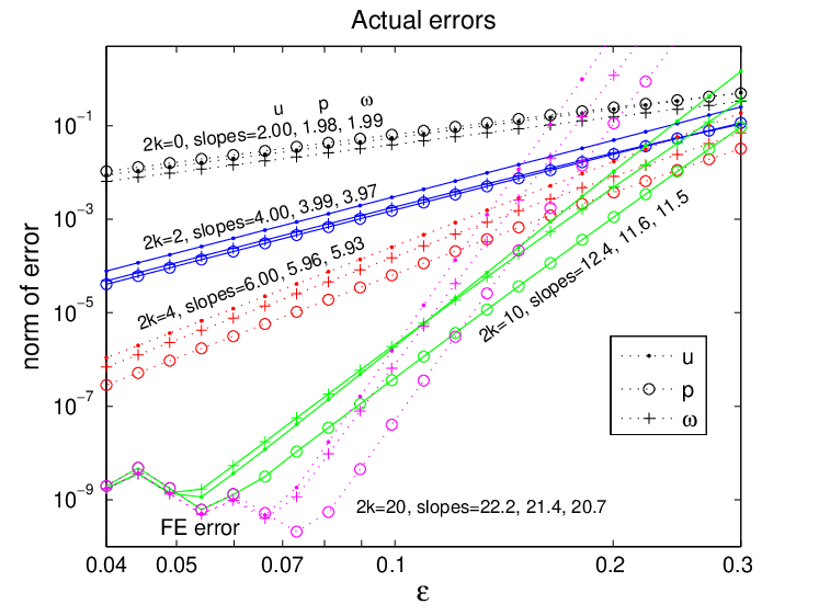
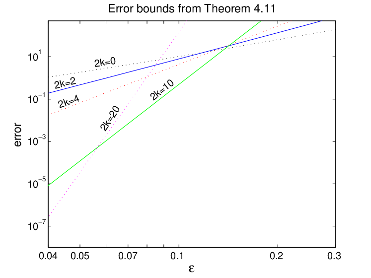
Refer to caption
Refer to caption
Fig. 5: Top: plot of ‖𝐮err(2​k)‖1,ε=(‖uerr(2​k)‖1,ε2+‖ε​verr(2​k)‖1,ε2)1/2\|\mathbf{u}_{\text{\it err}}^{(2k)}\|_{1,\varepsilon}=(\|u_{\text{\it err}}^{(2k)}\|_{1,\varepsilon}^{2}+\|\varepsilon v_{\text{\it err}}^{(2k)}\|_{1,\varepsilon}^{2})^{1/2}, ‖perr(2​k)‖0\|p_{\text{\it err}}^{(2k)}\|_{0}, and ‖ωerr(2​k)‖0\|\omega_{\text{\it err}}^{(2k)}\|_{0} for a=1/5a=1/5, 0.04≤ε≤0.30.04\leq\varepsilon\leq 0.3, and 2​k∈{0,2,4,10,20}2k\in\{0,2,4,10,20\}. The slopes of the lines were computed via linear regression using the smallest 1010 values of ε\varepsilon for which the finite element solution is trusted (ε≥0.066\varepsilon\geq 0.066 for 2​k=102k=10 and ε≥0.09\varepsilon\geq 0.09 for 2​k=202k=20). As expected, for fixed kk, the error is O⁡(ε2​k+2)O(\varepsilon^{2k+2}). Bottom: plot of the error bound (∗)(*) in (170), using V0=−.5V_{0}=-.5, V1=1V_{1}=1, I1=2.236I_{1}=2.236, I3=24.60I_{3}=24.60, and rk=0.3559r_{k}=0.3559 for k≥0k\geq 0, as appropriate for h⁡(x)h(x) in (172) with a=1/5a=1/5.
Refer to caption
Refer to caption
Refer to caption
Refer to caption
Refer to caption
Fig. 6: Contour plots of ωexact\omega_{\text{\it exact}}, ωerr(0)\omega_{\text{\it err}}^{(0)}, ωerr(4)\omega_{\text{\it err}}^{(4)}, ωerr(10)\omega_{\text{\it err}}^{(10)}, and ωerr(20)\omega_{\text{\it err}}^{(20)} for h⁡(x)h(x) in (172) with a=1/5a=1/5, V0=−0.5V_{0}=-0.5, V1=1.0V_{1}=1.0, and ε=0.099\varepsilon=0.099. Each of these plots corresponds to one of the markers in Figure 5.
Refer to caption
Refer to caption
Refer to caption
Refer to caption
Refer to caption
Fig. 7: Contour plots of pexactp_{\text{\it exact}}, perr(0)p_{\text{\it err}}^{(0)}, perr(4)p_{\text{\it err}}^{(4)}, perr(10)p_{\text{\it err}}^{(10)}, and perr(20)p_{\text{\it err}}^{(20)} for h⁡(x)h(x) in (172) with a=1/5a=1/5 and ε=0.099\varepsilon=0.099. The “exact” solution was computed using a least squares finite element method with 1515 node quartic triangular elements on a 2208×962208\times 96 grid.
Refer to caption
Fig. 8: Error estimates and actual errors with a=1/100a=1/100.
Refer to caption
Refer to caption
Refer to caption
Refer to caption
Fig. 9: Plots of ωexact\omega_{\text{\it exact}}, pexactp_{\text{\it exact}}, ωerr(10)\omega_{\text{\it err}}^{(10)}, and perr(10)p_{\text{\it err}}^{(10)} with a=1/100a=1/100, N=64N=64, M=4800M=4800.

The results are summarized in Figures 5–9. For 21 values of ε\varepsilon spaced exponentially between ε0=0.04\varepsilon_{0}=0.04 and ε20=0.3\varepsilon_{20}=0.3, we set up a logically rectangular, M×NM\times N finite element mesh on the domain

(173) Ωε={(x,y): 0≤x≤1,  0<y<εh(x)}.\Omega_{\varepsilon}=\{(x,y)\;:\;0\leq x\leq 1,\;\;0<y<\varepsilon h(x)\}.

The mesh points are aligned vertically with equal spacing Δ​y=h⁡(x)/N\Delta y=h(x)/N, while the grid spacing in the xx-direction is chosen to keep the aspect ratios of the grid cells as close to 1 as possible; we do this by solving an ODE to enforce Δ​x≈h⁡(x)/N\Delta x\approx h(x)/N, which also determines MM. For a=1/5a=1/5, we use N=96N=96 with MM ranging from 768 to 5376 as ε\varepsilon ranges from 0.30.3 to 0.040.04; for a=1/100a=1/100, we use N=64N=64 with MM ranging from 1600 to 10368. Four-by-four blocks of neighboring grid cells are merged and cut into two 15 node triangles. Interior nodes of the triangles are adjusted to keep the edges straight except on the top boundary, where we use quartic isoparametric elements. We solve the Stokes equations on this mesh using a least squares finite element method similar to [6] but using quartic elements to model the velocity components uu and vv, the pressure pp, the vorticity ω=vx−uy\omega=v_{x}-u_{y}, and two strain rates τ=uy+vx\tau=u_{y}+v_{x} and γ=vy−ux\gamma=v_{y}-u_{x}. We use multigrid to solve the resulting system of equations, which takes from 3 to 15 minutes on a 2.4 GHz desktop machine with 16 GB RAM.

Once the finite element solution is known at the grid points, we normalize the velocity, pressure, and vorticity as described in section 2 and rescale the domain from Ωε\Omega_{\varepsilon} to Ω\Omega. We then use the method described in Appendix A to compute ψ(0)\psi^{(0)}, ψ(2),…,ψ(20)\psi^{(2)},\dotsc,\psi^{(20)} and their derivatives through order 3 at the grid points. Next, we use the formulas in (31) to obtain u(2​k)u^{(2k)}, v(2​k)v^{(2k)}, ω(2​k)\omega^{(2k)}, and p(2​k)p^{(2k)} for k=0,…,10k=0,\dotsc,10. For pressure, we use 20 point Gaussian quadrature to integrate px(2​k)p_{x}^{(2k)} along the xx-axis to determine p(2​k)​(x,0)p^{(2k)}(x,0) at the mesh nodes. The integration of py(2​k)p_{y}^{(2k)} in the yy-direction is done analytically. With the expansion coefficients in hand, we evaluate

(174) uerr(2​k)\displaystyle u_{\text{\it err}}^{(2k)} =uexact−uapprox(2​k),\displaystyle=u_{\text{\it exact}}-u_{\text{\it approx}}^{(2k)}, uapprox(2​k)\displaystyle\quad u_{\text{\it approx}}^{(2k)} =u(0)+ε2​u(2)+⋯+ε2​k​u(2​k),\displaystyle=u^{(0)}+\varepsilon^{2}u^{(2)}+\cdots+\varepsilon^{2k}u^{(2k)},

etc., at the grid nodes, where we use the finite element solution for uexactu_{\text{\it exact}}. We then run through the triangles and sum up the local contributions to the errors

(175) ‖uerr(2​k)‖1,ε2+‖ε​verr(2​k)‖1,ε2,‖perr(2​k)‖02,‖ωerr(2​k)‖02\left\|u_{\text{\it err}}^{(2k)}\right\|_{1,\varepsilon}^{2}+\left\|\varepsilon v_{\text{\it err}}^{(2k)}\right\|_{1,\varepsilon}^{2},\qquad\left\|p_{\text{\it err}}^{(2k)}\right\|_{0}^{2},\qquad\left\|\omega_{\text{\it err}}^{(2k)}\right\|_{0}^{2}

by interpolating the values at the grid nodes and integrating the resulting polynomials on the triangle; this step is very similar to the assembly of the stiffness matrix. Finally, we store the results in a file for visualization (see Figures 6, 7, and 9) and record the norms of the truncation errors for comparison with the error bounds of Theorem 18.

The results of this comparison are shown in Figures 5 and 8. As expected, for fixed kk, the actual errors decay as O⁡(ε2​k+2)O(\varepsilon^{2k+2}). The a priori error bounds eventually decrease like O⁡(ε2​k+2)O(\varepsilon^{2k+2}) as well, but the term involving θk\theta_{k} in (170) is significant over this range of ε\varepsilon in some of the cases, causing the slopes to be larger:

θkrk​I3I1={k=0k=1k=2k=5k=10a=1/512.50.940.16.000961.3×10−11a=1/10025719.33.20.0202.7×10−10.\frac{\theta_{k}}{r_{k}}\sqrt{\frac{I_{3}}{I_{1}}}=\left\{\begin{array}[]{c|c|c|c|c|c}&k=0&k=1&k=2&k=5&k=10\\ \hline\cr a=1/5&12.5&0.94&0.16&.00096&1.3\times 10^{-11^{\phantom{1}}}\\ a=1/100&257&19.3&3.2&0.020&2.7\times 10^{-10^{\phantom{1}}}\end{array}.\right.

This effect is much more pronounced when a=1/100a=1/100 in (172) due to

(176) I3I1=12​32+1a+32​a2={3.32,a=1/5,61.4,a=1/100.\sqrt{\frac{I_{3}}{I_{1}}}=\frac{1}{2}\sqrt{\frac{3}{2}+\frac{1}{a}+\frac{3}{2a^{2}}}=\begin{cases}3.32,&a=1/5,\\ 61.4,&a=1/100.\end{cases}

The deviation from linearity in the plots of “actual error” for small ε\varepsilon and large kk is due to error in the finite element solutions, which are accurate to about 9 digits. This occurs sooner when a=1/100a=1/100 since the pressure and vorticity of the exact solution in the vicinity of the narrow gap increases as aa decreases, and also because we were forced to use a coarser mesh with a=1/100a=1/100 to avoid running out of computer memory in the finite element simulations. The data points with ε=0.099\varepsilon=0.099 in Figure 5 correspond to the contour plots in Figures 6 and 7, where we plot ωexact\omega_{\text{\it exact}}, ωerr(2​k)\omega_{\text{\it err}}^{(2k)}, pexactp_{\text{\it exact}}, and perr(2​k)p_{\text{\it err}}^{(2k)} for 2​k=0,4,10,202k=0,4,10,20. The data points with ε=0.099\varepsilon=0.099 in Figure 8 correspond to the contour plots in Figure 9. We remark that the apparently large value of perr(10)p_{\text{\it err}}^{(10)} in the narrow gap in Figure 9 is due to smoothing in the least squares finite element solver; the expansion solution is more accurate than the finite element solution in this region of the domain. The error patterns that emerge in all these cases are rather interesting, indicating that the spaces ℋ2​k\mathcal{H}_{2k} in Theorem 3 (the structure theorem) can be quite complicated even for simple curves h⁡(x)h(x).

Although our estimates for the error in pressure include an additional factor of h0−3/2(rk+rk−1)2h_{0}^{-3/2}(r_{k}+r_{k}^{-1})^{2}, all our numerical experiments (including complicated geometries in which the inf-sup constant β−1\beta^{-1} does exhibit h0−3/2h_{0}^{-3/2} behavior) indicate that ‖perr(2​k)‖0\|p_{\text{\it err}}^{(2k)}\|_{0} is comparable to ‖ωerr(2​k)‖0\|\omega_{\text{\it err}}^{(2k)}\|_{0}. In fact, for large kk, pressure seems to be the most accurately computed variable; see Figures 5 and 8. We do not know how to explain this as the pressure is determined by solving (151), which involves inverting the operator ∇:L#2​(Ω)→H−1​(Ω)2\nabla:L^{2}_{\#}(\Omega)\rightarrow H^{-1}(\Omega)^{2}. For some reason, in lubrication-type problems, the right-hand side 𝐟k\mathbf{f}_{k} belongs to a subspace of H−1​(Ω)2H^{-1}(\Omega)^{2} that is not amplified by (∇)−1(\nabla)^{-1} when solving ∇perr(2​k)=𝐟k\nabla p_{\text{\it err}}^{(2k)}=\mathbf{f}_{k}.

The following table shows the minimum ratio of the a priori error estimate to the actual error ‖𝐮err(2​k)‖1,ε\|\mathbf{u}_{\text{\it err}}^{(2k)}\|_{1,\varepsilon} for the data points in Figures 5 and 8 that were used to compute the slopes of the best-fit lines:

k=012510(min ratio, a=1/5)1/(2​k+2)​11.17.05.02.82.3(min ratio, a=1/100)1/(2​k+2)34.08.65.53.0−.\begin{array}[]{r|c|c|c|c|c}\lx@intercol\hfil k=\lx@intercol&0&1&2&5&10\\ \hline\cr\text{(min ratio, $a=1/5$)}^{1/(2k+2)}\rule{0.0pt}{12.0pt}&11.1&7.0&5.0&2.8&2.3\\ \text{(min ratio, $a=1/100$)}^{1/(2k+2)}&34.0&8.6&5.5&3.0&-\end{array}.

For example, in the 10 calculations (with ε\varepsilon ranging from 0.04≤ε≤0.0990.04\leq\varepsilon\leq 0.099) that were used to determine the slope of the 2​k=42k=4 line in Figure 5, the ratios of the a priori errors to the exact errors ranged between 1.608×1041.608\times 10^{4} and 1.617×1041.617\times 10^{4}, so we recorded 1.608×1046≈5.0\sqrt[6]{1.608\times 10^{4}}\approx 5.0. This table gives information on how far the values ρk\rho_{k} in Table 4 are from their optimal values. For example, if we increased ρ5\rho_{5} by more than a factor of 2.82.8 while holding θ5\theta_{5} fixed, the estimate (169) would fail to hold for this geometry. Since rk−1r_{k}^{-1} in (120) is used as a convenient upper bound on all the integrals |Em,j(2​ℓ)|1/2​ℓ|E_{m,j}^{(2\ell)}|^{1/2\ell} and |E~m,j(2​ℓ)|1/4​ℓ|\widetilde{E}_{m,j}^{(2\ell)}|^{1/4\ell} that arise in the definition of Q(2​k)Q^{(2k)} and also in the bounds for ‖ψx​x(2​k)‖0\|\psi^{(2k)}_{xx}\|_{0} and ‖h2​ψx​x​x​x(2​k−2)‖0\|h^{2}\psi^{(2k-2)}_{xxxx}\|_{0}, it is remarkable that the values of ρk\rho_{k} we computed are within a factor of 3 of optimal for k=5k=5, k=10k=10, and perhaps all k≥5k\geq 5.

6 Discussion

Although we are able to estimate the effective radius of convergence ρk​rk\rho_{k}r_{k} quite closely, our estimates of ‖ψerr(2​k)‖2,ε\|\psi_{\text{\it err}}^{(2k)}\|_{2,\varepsilon}, ‖ωerr(2​k)‖0\|\omega_{\text{\it err}}^{(2k)}\|_{0}, etc., are likely to be several orders of magnitude too large. One shouldn’t expect an a priori bound that holds for all geometries alike to provide an exceptionally sharp bound for any specific geometry. Instead, our analysis provides a clear picture of the features of h⁡(x)h(x) that cause the effective radii of curvature rk​ρkr_{k}\rho_{k} to become small, namely, large values of hk−1​∂xkhh^{k-1}\partial_{x}^{k}h. No previous study has ever described how the constant hidden in the O⁡(ε2​k+2)O(\varepsilon^{2k+2}) depends on hh; instead, hh has always been fixed at the outset and only the limit as ε→0\varepsilon\rightarrow 0 has been considered.

Refer to caption
Fig. 10: Comparison of uapprox(2​k)u_{\text{\it approx}}^{(2k)} (solid lines) to uexactu_{\text{\it exact}} (dots) at the point (x,y)=(38,34​h)(x,y)=(\frac{3}{8},\frac{3}{4}h) for 2​k=0,2,4,6,10,16,20,30,502k=0,2,4,6,10,16,20,30,50. Here h⁡(x)=35+25​sin⁡(2​π​x)h(x)=\frac{3}{5}+\frac{2}{5}\sin(2\pi x), V0=−0.5V_{0}=-0.5, and V1=1V_{1}=1. This function h⁡(x)h(x) is real analytic and periodic, yet the expansion solution appears to be an asymptotic series rather than a convergent series.

Another feature of this analysis is that it separates the constants into two types: those that are (1) given in the problem statement or easily computable from hh; or (2) difficult to compute but universal (independent of hh). We listed the first several constants in the latter category (ρk\rho_{k} and θk\theta_{k}) in Table 4. It is interesting that ρk\rho_{k} actually increases until 2​k=102k=10 and doesn’t get as bad as ρ0\rho_{0} again until 2​k=262k=26. However, at that point it seems to be decreasing steadily like 1/k1/k, indicating that the effective radius of curvature in our a priori error bound will shrink to zero as k→∞k\rightarrow\infty. The reason for this is that the recurrences (179) and (180) relating the matrices Ai(2​k)A_{i}^{(2k)} and B(2​k)B^{(2k)} to their lower order counterparts cause the norms of these matrices to grow like k!k!. Thus, although ρk\rho_{k} involves kkth roots of these constants, these kkth roots still grow linearly in kk. On the other hand, if hh is real analytic as well as periodic, a standard contour integral argument shows that there is an r>0r>0 such that ‖∂xkh‖∞≤k!​r−k\|\partial_{x}^{k}h\|_{\infty}\leq k!\,r^{-k} for all k≥0k\geq 0; thus, the constants rkr_{k} will remain bounded away from zero. For example, if h⁡(x)h(x) is of the form (172), one may show that if a∈(0,2/3]a\in(0,2/3], then the largest value of ‖1ℓ!​hℓ−1​∂xℓh‖∞1/ℓ\|\frac{1}{\ell!}h^{\ell-1}\partial_{x}^{\ell}h\|_{\infty}^{1/\ell} occurs when ℓ=2\ell=2, so all the rkr_{k} are equal to r0=(π​1−a)−1r_{0}=(\pi\sqrt{1-a})^{-1}. It is conceivable that when hh is real analytic, the norms of the functions ψ(2​k)\psi^{(2k)} grow slowly enough that the stream function expansion converges in spite of the fact that the matrices Ai(2​k)A_{i}^{(2k)} and B(2​k)B^{(2k)} in their representation (45) blow up like k!k!. This would simply mean that we chose a bad basis in terms of which to represent ψ\psi. We used orthogonal polynomials in (136) to improve this basis, but there may be other improvements. Figure 10 shows that this is not the case. Even when hh varies sinusoidally, the expansion solution appears to be an asymptotic series rather than a convergent series: all the variables, including the flux terms Q(2​k)Q^{(2k)}, appear to grow like k!k! as kk becomes large.

Nevertheless, the expansion solutions can be extremely accurate (almost exact) as long as they are used for a geometry that falls within the effective radius of convergence of the truncated series. It is hoped that the estimates in this paper will help to identify these cases and provide practical a priori (as well as a posteriori) error estimates for many interesting problems.

Appendix A Implementation

We have developed two methods for computing the higher order corrections described in section 3.2 using a computer. In the first, we use Mathematica to evaluate the derivatives and antiderivatives in recursion (29) and Algorithm 1 symbolically. With this approach, the main challenge occurs at the step where Q(2​k0)Q^{(2k_{0})} is defined as a definite integral. We do this through pattern matching and symbol replacement. At the stage where the definite integral is to be evaluated, we replace all instances of ∂xjh\partial_{x}^{j}h in the integrand by j!​tj/hj−1j!\,t_{j}/h^{j-1}. Each term in the result (call it RR) will contain a factor of h−3h^{-3} or h−2h^{-2}, with no other dependence

on hh. For each k=k0,…,0k=k_{0},\dotsc,0 and j=1,…,d2​kj=1,\dotsc,d_{2k}, we find the terms in RR that contain φj(2​k)\varphi^{(2k)}_{j} (left in the form t1i1⋯t2​ki2​kt_{1}^{i_{1}}\cdots t_{2k}^{i_{2k}} described in Algorithm 2) as a factor. These terms are removed from RR while their symbolic integrals (with φj(2​k)/hm\varphi^{(2k)}_{j}/h^{m} replaced by Im​Em,j(2​k)I_{m}E^{(2k)}_{m,j}) are divided by 2​I32I_{3} and added to the desired flux Q(2​k0)Q^{(2k_{0})}. By running through the φj(2​k)\varphi^{(2k)}_{j} in decreasing kk order, we convert higher order products (e.g., t12​t2/h3t_{1}^{2}t_{2}/h^{3}) into symbols (e.g., I3​E3,2(4)I_{3}E^{(4)}_{3,2}) before one of their lower order factors can be converted incorrectly (e.g., into I3​E3,1(2)​t2I_{3}E^{(2)}_{3,1}t_{2}). This approach is effective through 6th or 8th order but becomes rather slow as the complexity of the expansion increases.

The second approach is much faster and can be implemented in any modern programming language. We have written a version in C+⁣+C^{++} and a version in Mathematica. Instead of representing the basis functions φj(k)\varphi^{(k)}_{j} for ℋk\mathcal{H}_{k} using a computer algebra system, we represent them as (k+1)(k+1)-tuples of integers. For example, the functions 11, hxh_{x}, 16​h2​hx3​hx​x​x\frac{1}{6}h^{2}h_{x}^{3}h_{xxx}, and 148​h4​hx​hx​x​hx​x​x​x\frac{1}{48}h^{4}h_{x}h_{xx}h_{xxxx} in ℋ0\mathcal{H}_{0}, ℋ1\mathcal{H}_{1}, ℋ6\mathcal{H}_{6}, and ℋ7\mathcal{H}_{7} are represented by (0)(0), (0,1)(0,1), (2,3,0,1,0,0,0)(2,3,0,1,0,0,0), and (4,1,1,0,1,0,0,0)(4,1,1,0,1,0,0,0). A tuple (i0,…,ik)(i_{0},\dotsc,i_{k}) represents a basis function for ℋk\mathcal{H}_{k} iff

(177) i1+2​i2+⋯+k​ik=k,i0=i2+2​i3+⋯+(k−1)​ik.i_{1}+2i_{2}+\cdots+ki_{k}=k,\qquad i_{0}=i_{2}+2i_{3}+\cdots+(k-1)i_{k}.

We begin by constructing the basis sets Φk\Phi_{k} for 0≤k≤2​k00\leq k\leq 2k_{0} and storing them as (k+1)×dk(k+1)\times d_{k} integer matrices with columns corresponding to the φj(k)\varphi^{(k)}_{j}. This is done using Algorithm 2, which returns the columns sorted lexicographically from the last slot to the first slot (e.g., (3,0,3,0)T<(2,3,0,1)T<(3,1,1,1)T(3,0,3,0)^{T}<(2,3,0,1)^{T}<(3,1,1,1)^{T}). Sorted columns allow us to find the column index corresponding to a given tuple in log2⁡dk\log_{2}d_{k} time.

Next, for 0≤k≤2​k0−10\leq k\leq 2k_{0}-1, we compute the operators h∂xh\partial_{x} and hx⋅h_{x}\cdot from ℋk\mathcal{H}_{k} to ℋk+1\mathcal{H}_{k+1} and store them as sparse integer matrices of dimension dk+1×dkd_{k+1}\times d_{k}. If column JJ of Φk\Phi_{k} contains the tuple (i0,…,ik)(i_{0},\dotsc,i_{k}), we define ik+1=0i_{k+1}=0 and compute

(178) hx⋅:(i0,…,ik)\displaystyle h_{x}\cdot:(i_{0},\dotsc,i_{k}) ↦(i0,i1+1,i2,…,ik+1),\displaystyle\mapsto(i_{0},i_{1}+1,i_{2},\dotsc,i_{k+1}),
h∂x:(i0,…,ik)\displaystyle h\partial_{x}:(i_{0},\dotsc,i_{k}) ↦∑{r:ir≠0}ir(r+1)(i0+1,…,ir−1,ir+1+1,…,ik+1),\displaystyle\mapsto\sum_{\{r\,:\,i_{r}\neq 0\}}i_{r}(r+1)(i_{0}+1,\dotsc,i_{r}-1,i_{r+1}+1,\dotsc,i_{k+1}),

where the omitted indices are unmodified and the +1+1 and −1-1 cancel in the first slot when r=0r=0 in the sum. The factor of (r+1)(r+1) is due to the factorials in the definition of the φj(k)\varphi^{(k)}_{j}. The column index ll of each (k+2)(k+2)-tuple in the result is found in Φk+1\Phi_{k+1}, and the corresponding coefficient (1 or ir​(r+1)i_{r}(r+1)) is added to the llth row and JJth column of the sparse matrix representing h∂xh\partial_{x} or hx⋅h_{x}\cdot. The entries of these sparse matrices are positive, and the column sums (i.e., 1-norms) are all equal to 11 for hx⋅h_{x}\cdot and to i0+2​i1+⋯+(k+1)​ik=2​ki_{0}+2i_{1}+\cdots+(k+1)i_{k}=2k for h∂xh\partial_{x} (by (177)).

Once the operators h∂xh\partial_{x} and hx⋅h_{x}\cdot are known, we use them to recursively compute the matrices A(2​k)=V0​A0(2​k)+V1​A1(2​k)A^{(2k)}=V_{0}A_{0}^{(2k)}+V_{1}A_{1}^{(2k)} and B(2​k)B^{(2k)} in (45). We start by setting A0(0)=(0,1,−2,1)TA_{0}^{(0)}=(0,1,-2,1)^{T}, A1(0)=(0,0,−1,1)TA_{1}^{(0)}=(0,0,-1,1)^{T}, and B(0)=(0,0,3,−2)TB^{(0)}=(0,0,3,-2)^{T} as in Example 5. For 1≤k≤k01\leq k\leq k_{0}, we mimic the proof of Theorem 3 to build up A(2​k)A^{(2k)} and B(2​k)B^{(2k)} row by row. For 4≤n≤2​k+34\leq n\leq 2k+3 and i=0,1i=0,1, we use sparse matrix–vector multiplication to define the rows

(179) Ai(2​k)(n,:)\displaystyle A_{i}^{(2k)}(n,:) =(−2[h∂x−(n−2)hx][h∂x−(n−3)hx][Ai(2​k−2)(n,:)T]n⁡(n−1))T,\displaystyle=\left(\frac{-2[h\partial_{x}-(n-2)h_{x}][h\partial_{x}-(n-3)h_{x}]\left[A_{i}^{(2k-2)}(n,:)^{T}\right]}{n(n-1)}\right)^{T},
B(2​k)(n,:)\displaystyle B^{(2k)}(n,:) =(−2[h∂x−(n−1)hx][h∂x−(n−2)hx][B(2​k−2)(n,:)T]n⁡(n−1))T.\displaystyle=\left(\frac{-2[h\partial_{x}-(n-1)h_{x}][h\partial_{x}-(n-2)h_{x}]\left[B^{(2k-2)}(n,:)^{T}\right]}{n(n-1)}\right)^{T}.

If k≥2k\geq 2, then for 6≤n≤2​k+36\leq n\leq 2k+3, we add the following vectors to Ai(2​k)(n,:)A_{i}^{(2k)}(n,:) and B(2​k)(n,:)B^{(2k)}(n,:), respectively:

(180) (−[h∂x−(n−2)hx][h∂x−(n−3)hx][h∂x−(n−4)hx][h∂x−(n−5)hx][Ai(2​k−4)(n,:)T]n⁡(n−1)​(n−2)​(n−3))T,\displaystyle\textstyle\displaystyle\left(\hskip-2.0pt\frac{-[h\partial_{x}-(n-2)h_{x}][h\partial_{x}-(n-3)h_{x}][h\partial_{x}-(n-4)h_{x}][h\partial_{x}-(n-5)h_{x}]\left[A_{i}^{(2k-4)}(n,:)^{T}\right]}{n(n-1)(n-2)(n-3)}\hskip-1.0pt\right)^{T}\hskip-3.0pt,
(−[h∂x−(n−1)hx][h∂x−(n−2)hx][h∂x−(n−3)hx][h∂x−(n−4)hx][B(2​k−4)(n,:)T]n⁡(n−1)​(n−2)​(n−3))T.\displaystyle\textstyle\displaystyle\left(\hskip-2.0pt\frac{-[h\partial_{x}-(n-1)h_{x}][h\partial_{x}-(n-2)h_{x}][h\partial_{x}-(n-3)h_{x}][h\partial_{x}-(n-4)h_{x}]\left[B^{(2k-4)}(n,:)^{T}\right]}{n(n-1)(n-2)(n-3)}\hskip-1.0pt\right)^{T}\hskip-3.0pt.

Next we zero out rows 0 and 1 of A0(2​k)A_{0}^{(2k)}, A1(2​k)A_{1}^{(2k)}, B(2​k)B^{(2k)}, and set

(181) Ai(2​k)(2,:)\displaystyle A_{i}^{(2k)}(2,:) =∑n=42​k+3(n−3)Ai(2​k)(n,:),Ai(2​k)(3,:)=∑n=42​k+3(2−n)Ai(2​k)(n,:),\displaystyle=\sum_{n=4}^{2k+3}(n-3)A_{i}^{(2k)}(n,:),\quad A_{i}^{(2k)}(3,:)=\sum_{n=4}^{2k+3}(2-n)A_{i}^{(2k)}(n,:),
B(2​k)(2,:)\displaystyle B^{(2k)}(2,:) =∑n=42​k+3(n−3)B(2​k)(n,:),B(2​k)(3,:)=∑n=42​k+3(2−n)B(2​k)(n,:).\displaystyle=\sum_{n=4}^{2k+3}(n-3)B^{(2k)}(n,:),\quad B^{(2k)}(3,:)=\sum_{n=4}^{2k+3}(2-n)B^{(2k)}(n,:).

Finally, we subtract (−1/2k){-1/2\choose k} from A1(2​k)​(2,1)A_{1}^{(2k)}(2,1) and add it to A1(2​k)​(3,1)A_{1}^{(2k)}(3,1) to account for the boundary data, where we recall that the rows and columns are indexed starting at 0 and 1, respectively. Using this approach, our C+⁣+C^{++} code can compute these matrices through order 2​k=502k=50 using floating point arithmetic in a few seconds, while our Mathematica code can compute through order 2​k=302k=30 in exact rational arithmetic in about an hour. This allows us to explore the properties of the stream function expansion and test our error estimates to quite a high order.

References

  • [1] M. Abramowitz and I. A. Stegun, Handbook of Mathematical Functions with Formulas, Graphs, and Mathematical Tables, Dover, New York, 1964.
  • [2] A. Assemien, G. Bayada, and M. Chambat, Inertial effects in the asymptotic behavior of a thin film flow, Asympt. Anal., 9 (1994), pp. 177–208.
  • [3] G. Bayada and M. Chambat, The transition between the Stokes equations and the Reynolds equation: A mathematical proof, Appl. Math. Optim., 14 (1986), pp. 73–93.
  • [4] G. Bayada and M. Chambat, Modélisation de la jonction d’un écoulement tridimensionnel et d’un film mince bidimensionnel, C. R. Acad. Sci. Paris, Ser. I, 309 (1989), pp. 81–84.
  • [5] D. Braess, Finite Elements—Theory, Fast Solvers, and Applications in Solid Mechanics, Cambridge University Press, Cambridge, UK, 1997.
  • [6] Z. Cai, T. A. Manteuffel, and S. F. McCormick, First-order system least squares for the Stokes equations, with application to linear elasticity, SIAM J. Numer. Anal., 34 (1997), pp. 1727–1741.
  • [7] E. V. Chizhonkov and M. A. Olshanskii, On the domain geometry dependence of the LBB condition, M2AN Math. Model. Numer. Anal., 34 (2000), pp. 935–951.
  • [8] G. Cimatti, How the Reynolds equation is related to the Stokes equations, Appl. Math. Optim., 10 (1983), pp. 267–274.
  • [9] I. Ciuperca, I. Hafidi, and M. Jai, Singular perturbation problem for the incompressible Reynolds equation, Electron. J. Differential Equations, 2006 (2006), pp. 1–19.
  • [10] M. Dobrowolski, On the LBB constant on stretched domains, Math. Nachr., 254–255 (2003), pp. 64–67.
  • [11] A. Duvnjak and E. Marus̆ić-Paloka, Derivation of the Reynolds equation for lubrication of a rotating shaft, Arch. Math., 36 (2000), pp. 239–253.
  • [12] H. G. Elrod, A derivation of the basic equations for hydrodynamic lubrication with a fluid having constant properties, Quart. Appl. Math., XVII (1960), pp. 349–359.
  • [13] G. P. Galdi, An Introduction to the Mathematical Theory of the Navier-Stokes Equations, Vol. 1: Linearized Steady Problems, Springer–Verlag, New York, 1994.
  • [14] V. Girault and P.-A. Raviart, Finite Element Methods for Navier–Stokes Equations, Springer–Verlag, Berlin, 1986.
  • [15] J. Kevorkian and J. D. Cole, Multiple Scale and Singular Perturbation Methods, Springer-Verlag, New York, 1996.
  • [16] W. E. Langlois, Slow Viscous Flow, Macmillan, New York, 1964.
  • [17] I. Moise, R. Temam, and M. Ziane, Asymptotic analysis of the Navier-Stokes equations in thin domains, Topol. Methods Nonlinear Anal., 10 (1997), pp. 249–282.
  • [18] S. A. Nazarov, Asymptotic solution of the Navier-Stokes problem on the flow of a thin layer of fluid, Siberian Math. J., 31 (1990), pp. 296–307.
  • [19] S. A. Nazarov, Asymptotics of the Stokes system solutions at a surfaces contact point, C. R. Acad. Sci. Paris, Sér. I, 312 (1991), pp. 207–211.
  • [20] C. Pozrikidis, Introduction to Theoretical and Computational Fluid Dynamics, Oxford University Press, New York, 1997.
  • [21] G. Raugel and G. R. Sell, Navier-Stokes equations on thin 33D domains. I: Global attractors and global regularity of solutions, J. Amer. Math. Soc., 6 (1993), pp. 503–568.
  • [22] O. Reynolds, On the theory of lubrication and its applications to Mr. Beauchamp Tower’s experiments, including an experimental determination of the viscosity of olive oil, Philos. Trans. R. Soc. Lond., 177 (1886), pp. 157–234.
  • [23] G. Stoyan, Iterative Stokes solvers in the harmonic Velte subspace, Computing, 67 (2001), pp. 13–33.
  • [24] J. Wilkening, Inf-sup estimates for the Stokes problem in a periodic channel, arXiv:0706.4082.
  • [25] J. Wilkening and A. E. Hosoi, Shape optimization of a sheet swimming over a thin liquid layer, J. Fluid Mech., 601 (2008), pp. 25–61.