1Introduction

FIT HE-07-01

MPP-2007-74

Holographic heavy-light mesons

from non-Abelian DBI

Johanna Erdmenger ^a ²² 2 jke@mppmu.mpg.de, Kazuo Ghoroku ^b ¹¹ 1 gouroku@dontaku.fit.ac.jp and Ingo Kirsch ^c ³³ 3 kirsch@phys.ethz.ch

^a Max Planck-Institut für Physik (Werner Heisenberg-Institut), Föhringer Ring 6, 80805 München, Germany

^bFukuoka Institute of Technology, Fukuoka 811-0295, Japan

^c Institut für Theoretische Physik, ETH Zürich,
CH-8093 Zürich, Switzerland

In the context of gauge/gravity duals with flavor, we examine heavy-light mesons which involve a heavy and a light quark. For this purpose we embed two D7 brane probes at different positions into the gravity background. We establish the non-Abelian Dirac-Born-Infeld (DBI) action for these probes, in which the $U(2)$ matrix describing the embedding is diagonal. The fluctuations of the brane probes correspond to the mesons. In particular, the off-diagonal elements of the $U(2)$ fluctuation matrix correspond to the heavy-light mesons, while the diagonal elements correspond to the light-light and heavy-heavy mesons, respectively. The heavy-light mesons scale differently with the ’t Hooft coupling than the mesons involving quarks of equal mass. The model describes both scalar and vector mesons. For different dilaton-deformed gravity backgrounds, we also calculate the Wilson loop energy, and compare with the meson masses.

1 Introduction

Recently, based on the gauge/gravity correspondence [1], many non-perturbative properties of Yang-Mills theories with quarks have been uncovered in terms of superstring theory [2]-[11]. Flavor quarks in the fundamental representation of the gauge group are introduced by embedding one or several probe branes into an appropriate bulk gravity background, in order to describe large $N$ gauge theories similar to QCD. Many successful results have been obtained for the properties of quarks and their bound states: Mesons spectra have been studied by many authors, including [3]-[20]. The mass spectra of fermionic operators with fundamental fields (“mesinos”) have been discussed in [21, 22].

Up to now, most of these investigations have been devoted to the case that the D7 branes are embedded at the same place, such that the flavor group forms $U(N_{f})$ for $N_{f}$ D7 branes. Effects of the non-abelian nature of $U(N_{f})$ for $N_{f}>1$ in relation to bulk instantons have been studied in [23] and in [24]-[26]. Examples of D7 branes embedded at different positions occur in studies of meson decay via string breaking [27]-[29].

Here we propose a holographic model for heavy-light mesons based on a non-abelian Dirac-Born-Infeld (DBI) action. In this model, two D7 brane probes are embedded at different positions, such that they provide different quark mass states depending on the flavor. It is possible to choose any mass difference by separating the branes by an appropriate distance. In terms of this model, we study meson states with heavy and light quarks, such as mesons with charm or bottom degrees of freedom for instance. Heavy-light mesons with large spin have been studied in [30, 31].

In [32], an effective model for heavy-light mesons such as the B meson has been proposed which is based on the Polyakov action. This model gives a qualitative description of the B and excited B^∗ states. It also gives rise to a dependence of the heavy-light meson mass on the ’t Hooft coupling ( $\lambda$ ) of the form $M_{HL}/m_{H}=1+{\rm const}/\sqrt{\lambda}+{\cal O}(\lambda^{-1})$ , with $M_{HL}$ the heavy-light meson mass and $m_{H}$ the heavy quark mass (The light quark mass $m_{L}$ has been set to zero here.). This differs from the ’t Hooft coupling dependence of the light-light or heavy-heavy mesons [3], for which $M\propto m/\sqrt{\lambda}$ . However the result of [32] ensures that the heavy-light meson mass equals the heavy quark mass in the large $\lambda$ limit, $M_{HL}=m_{H}$ , as expected from observation and dimensional analysis.

Here we present an alternative approach to the same heavy-light meson mass in terms of a non-Abelian Dirac-Born-Infeld (DBI) action for two D7 branes at different positions. We use the non-Abelian DBI action for curved 10d backgrounds which has been proposed by Myers [33]. In this action, the world-volume fields are assigned to $U(N_{f})$ matrix-valued functions for $N_{f}$ D7 branes. We choose $N_{f}=2$ . The embedding configuration of the two D7 branes is determined by the diagonal components of the scalar fields. The corresponding equation of motion is solved by the profile functions of two separated branes, one of which corresponds to the heavy and one to the light quark. The quark masses are given by the boundary values of the two embedded branes. The fluctuations of the diagonal elements of the $2\times 2$ flavor matrices correspond to the light-light and heavy-heavy mesons, respectively. On the other hand, the off-diagonal components of the fluctuations of the fields on the branes are identified with the heavy-light mesons. We calculate the spectrum of these heavy-light mesons.

For the $\lambda$ dependence of the heavy-light meson mass, we find that it is similar to the one observed using the Polyakov action approach in [32]. A finite contribution to the mass remains in the limit of $\lambda\to\infty$ . This contribution corresponds to the minimum energy of a classical string connecting two separated D7 branes, and thus is equivalent to the mass obtained from the Polyakov action.

This $\lambda$ dependence persists if we consider the ${\rm D3}+{\rm D(-1)}$ gravity background of [34]. In the field theory dual to this background, a condensate $q\equiv\pi^{2}\langle F^{2}\rangle$ is switched on. D7 embeddings and chiral symmetry breaking for a non-supersymmetric version of this background have been studied in [10]. The $\lambda$ dependence is very similar to that in the supersymmetric background.

It is instructive to compare the $\lambda$ dependence of the meson spectra with the $\lambda$ dependence of the tension. For a classical string stretched between the two D7 brane probes, the string tension is independent of $\lambda$ , in agreement with the heavy-light meson mass result found in [32] as well as in the present paper. For heavy-light mesons this tension contributes to the meson mass even if the distance $L$ between the quark and anti-quark in the four-dimensional boundary space is zero, in which case it contributes $E=m_{H}-m_{L}$ to the Wilson line energy. For the heavy-heavy and light-light mesons, the string tension scales as $m_{q}^{2}/\sqrt{\lambda}$ for small $L$ [3, 10]. At large $L$ , when the dual gauge theory is in the quark confinement phase, there is a long range linear potential for all the mesons considered. For the heavy-heavy and light-light mesons this was found in [10].

Our model allows to describe both scalar and vector mesons. In this respect, it goes beyond the effective model of [32]. For the supersymmetric ${\rm D3}+{\rm D(-1)}$ background of [34], we find that the vector and scalar meson masses differ, due to the different dependence of the fluctuation equations on the non-trivial dilaton. Note that when adding D7 probes to the ${\rm D3}+{\rm D(-1)}$ background, supersymmetry is broken to ${\cal N}=1$ and the vector and scalar mesons are not in the same multiplet any more. For very large heavy quark mass, ${\cal N}=2$ supersymmetry is restored, and the vector and scalar meson masses become degenerate again. This is consistent with the phenomenological fact from heavy-quark theory that spin effects are suppressed by powers of the inverse heavy quark mass. Of course, here this is due to ${\cal N}=2$ supersymmetry restoration. We leave an investigation of this mechanism for non-supersymmetric backgrounds to the future.

Our paper is organized as follows. In section 2, we give the non-Abelian DBI action and the D7 brane embedding model is proposed. In section 3, the number of D7 branes is restricted to two ( $N_{f}=2$ ) and the action is expanded by fluctuations to see the meson spectra, which are shown in the section 4 for the case of HL mesons. In section 5, the potential between quark and anti-quark is given through Wilson loop. The summary is given in the final section.

2 Embedding of D7 branes

2.1 Non-Abelian Dirac-Born-Infeld action

We start from the non-Abelian Dirac-Born-Infeld action proposed by Myers in [33]. This action describes the dynamics of $N_{f}$ D $p$ -branes in a background with metric $G_{mn}$ and is given by

\displaystyle S_{N_{f}}=-\tau_{p}\int d^{p+1}\xi e^{-\phi}{\,\rm STr}\left(\sqrt{-\det(P[G_{rs}+G_{ra}(Q^{-1}-\delta)^{ab}G_{sb}]+T^{-1}F_{rs})}\sqrt{\det Q^{a}{}_{b}}\right)\,,

(1)

where the matrix $Q^{a}{}_{b}$ is defined by

Q^{a}{}_{b}=\delta^{a}{}_{b}+iT[X^{a},X^{c}]G_{cb}\,

(2)

where $T^{-1}=2\pi\alpha^{\prime}$ , and $X^{a}$ are the coordinates transverse to the stack of branes, which now take values in a $U(N_{f})$ algebra. The symbol ${\rm STr}$ denotes the symmetrized trace ${\rm STr}(A_{1}...A_{n})\equiv\frac{1}{n!}{\rm Tr}(A_{1}...A_{n}$ + all permutations) and is needed to avoid the ambiguity of the ordering of the expansion of all fields in the DBI action. [35].

In our convention, $r,s=0,1,...,p$ and $a,b=p+1,...,9$ label the world-volume directions and the directions transverse to the D $p$ -branes, respectively; $m,n=0,1,\cdots,9$ are the 10d spacetime indices. $P[a_{rs}]$ denotes the pull-back of a 10d tensor $a_{mn}$ to the world-volume of the branes. A peculiarity of the non-Abelian DBI action is that the pull-back matrix is given by the covariant derivative

D_{r}X^{a}=\partial_{r}X_{a}+i[A_{r},X^{a}]\ ,

(3)

with partial derivatives $\partial_{r}\equiv\partial/\partial\xi^{r}$ , non-Abelian world-volume gauge field $A_{r}$ and transverse coordinates $X^{a}$ . $F_{rs}$ is the corresponding world-volume field strength.

For diagonal brane embeddings the commutator $[X^{a},X^{b}]$ is small, as can be seen as follows. Set $X^{a}$ as $X^{a}=\bar{X}^{a}+\phi^{a}$ , where $\phi^{a}$ denotes small quantum fluctuations around a diagonal embedding matrix $\bar{X}^{a}$ . Then we have

\displaystyle[X^{a},X^{b}]=[\bar{X}^{a},\bar{X}^{b}]+[\bar{X}^{a},\phi^{b}]+[\phi^{a},\bar{X}^{b}]+[\phi^{a},\phi^{b}]\,,

(4)

where the first term $[\bar{X}^{a},\bar{X}^{b}]$ vanishes and the remaining terms are small. Next, assuming also a diagonal metric $G_{mn}$ and employing the approximation $(Q^{-1}-\delta)^{ab}\approx-iT[X^{a},X^{b}]$ , we rewrite the pull-back in the action (1) as

\displaystyle P[G_{rs}+G_{ra}(Q^{-1}-\delta)^{ab}G_{sb}]\,\approx\,G_{rs}+D_{r}X^{a}D_{s}X^{b}\left(G_{ab}-iT[X^{c},X^{d}]G_{ac}G_{bd}\right)\,.

(5)

Then, the action (1) is expanded in powers of $[X^{a},X^{b}]$ up to $O\!\left(X^{4}\right)$ as

S_{N_{f}}=\tau_{p}\int d^{p+1}\xi\ e^{-\Phi}{\rm STr}\left\{\sqrt{-\det({G}_{rs}+G_{ab}D_{r}X^{a}D_{s}X^{b}+T^{-1}F_{rs})}\right.

\times\left.\left(1-{1\over 4}\left(TG_{ac}[X^{c},X^{b}]\right)^{2}\right)\ \right\}\ .

(6)

The factor in the second line descends from the expansion of $\sqrt{\det Q^{a}{}_{b}}$ . For a flat spacetime background $G_{mn}=\eta_{mn}$ , the action (6) agrees with that found in [35].

2.2 Diagonal embedding ansatz in non-Abelian DBI action

The non-Abelian DBI action will now be used to find the embedding of $N_{f}$ probe D7 branes in different gravity backgrounds. The embedding profiles correspond to the classical solutions for the scalar fields in the D7 brane action. In our case, the scalar fields $X^{a}$ are $U(N_{f})$ matrix valued functions which makes it difficult to obtain a general form of the profile functions. In order to simplify the problem, we use the diagonal ansatz

X^{a}={\rm diag}(w_{1}^{a},\cdots,w_{N_{f}}^{a})\,,

(7)

thereby setting all off-diagonal components to zero. Here each of the functions $w_{i}^{a}$ corresponds to one of the $N_{f}$ D7 branes. – It would be an interesting problem to also include the off-diagonal components of $X^{a}$ and to solve the corresponding embedding equations. For example, for a non-trivial world-volume gauge field $F_{rs}$ the off-diagonal components provide a BI-on configuration which connects two branes [36]. We postpone the discussion of such configurations to the future.

The quark mass for each flavor is given by the asymptotic value of $w_{i}^{a}$ in the ultraviolet limit. They are the integration constants and given by hand as parameters of the theory.^*^* * The asymptotic values of (possible) off-diagonal components, say $w_{ij}^{a}$ , represent the mass-mixing of different quark flavors $i$ and $j$ . We neglect these here. The equations of motion for the $w_{i}^{a}$ are obtained from the action

	$\displaystyle S_{N_{f}}$	$\displaystyle=\tau_{7}\int d^{8}\xi\ e^{-\Phi}{\rm STr}\left(\sqrt{-\det({G}_{rs}+G_{ab}\partial_{r}w_{i}^{a}\partial_{s}w_{i}^{b})}\right)$
		$\displaystyle=\tau_{7}\int d^{8}\xi\ e^{-\Phi}\sum_{i=1}^{N_{f}}\sqrt{-\det({G}_{rs}+G_{ab}\partial_{r}w_{i}^{a}\partial_{s}w_{i}^{b})}\,$		(8)

which is Eq. (6) for the embedding (7) and $p=7$ . The essential point is here that for the diagonal ansatz (7), we obtain $N_{f}$ decoupled equations of motion for the $w_{i}^{a}$ such that the embeddings of each of the probe branes is independent of the other. In other words, for diagonal embeddings the non-Abelian DBI action reduces to the sum of $N_{f}$ abelian DBI actions.^†^† † This is only true, if we ignore the fluctuations around the brane embeddings. As we will see in Sec. 3, the non-Abelian DBI action also describes fluctuations of strings stretched in between two different branes.

If there are additional fluxes in the background, the action (8) must be supplemented by appropriate Wess-Zumino terms.

2.3 Specific gravity background

Let us now find the embedding functions $w\equiv w_{i}$ ( $i=1,...,N_{f}$ ) of the probe branes for some phenomenologically interesting supergravity backgrounds.

As a specific supergravity background, we consider the following 10d background in string frame given by a non-trivial dilaton $\Phi$ and axion $\chi$ [34, 10],

ds^{2}_{10}=e^{\Phi/2}\left(\frac{r^{2}}{R^{2}}A^{2}(r)\eta_{\mu\nu}dx^{\mu}dx^{\nu}+\frac{R^{2}}{r^{2}}dr^{2}+R^{2}d\Omega_{5}^{2}\right)\ .

(9)

Here two typical solutions are considered. One is the supersymmetric solution

A=1,\quad e^{\Phi}=1+\frac{q}{r^{4}}\ ,\quad\chi=-e^{-\Phi}+\chi_{0}\ ,

(10)

and the other is non-supersymmetric and given by

A(r)=\left(1-(\frac{r_{0}}{r})^{8}\right)^{1/4},\quad\chi=0\ ,\quad e^{\Phi}=\left(\frac{(r/r_{0})^{4}+1}{(r/r_{0})^{4}-1}\right)^{\sqrt{3/2}}\ .

(11)

The first solution is dual to ${\cal N}=2$ super Yang-Mills theory with gauge condensate $q$ and is chirally symmetric. Both supersymmetry and chiral symmetry are broken for the second solution [10].

In order to obtain the induced metric on the D7 world-volume, we rewrite the six-dimensional part of the metric (9) in the form

\frac{R^{2}}{r^{2}}dr^{2}+R^{2}d\Omega_{5}^{2}=\frac{R^{2}}{r^{2}}\left(d\rho^{2}+\rho^{2}d\Omega_{3}^{2}+(dX^{8})^{2}+(dX^{9})^{2}\right)\ ,

(12)

where $r^{2}=\rho^{2}+(X^{8})^{2}+(X^{9})^{2}$ . Due to the rotational invariance in the $X^{8}-X^{9}$ plane, we may set $X^{8}=0$ and $X^{9}=w(\rho)$ without loss of generality. Then the induced metric on the D7 brane is given by

ds^{2}_{8}=e^{\Phi/2}\left\{{r^{2}\over R^{2}}A^{2}\eta_{\mu\nu}dx^{\mu}dx^{\nu}+\right.\left.\frac{R^{2}}{r^{2}}\left((1+(\partial_{\rho}w)^{2})d\rho^{2}+\rho^{2}d\Omega_{3}^{2}\right)\right\}\ .

(13)

In static gauge the action for the D7 probe is given by

S_{\rm D7}=S_{DBI}+S_{WZ}=-\tau_{7}~\int d^{8}\xi\sqrt{\epsilon_{3}}\rho^{3}\left(A^{4}e^{\Phi}\sqrt{1+(w^{\prime})^{2}}-C_{8}\right)\ ,

(14)

where $C_{8}=q/r^{4}=e^{\Phi}-1$ denotes the Wess-Zumino term coming from $A_{8}$ , the Hodge dual of the axion [10]. The Wess-Zumino term is only required for the supersymmetric background (10). The equation of motion for the embedding function $w(\rho)$ is

	$\displaystyle-{w\over\rho+w~w^{\prime}}\sqrt{1+(w^{\prime})^{2}}(\Phi+4\log A)^{\prime}$
	$\displaystyle\quad+{1\over\sqrt{1+(w^{\prime})^{2}}}\left[w^{\prime}\left({3\over\rho}+(\Phi+4\log A)^{\prime}\right)+{w^{\prime\prime}\over 1+(w^{\prime})^{2}}\right]=0$		(15)

for the non-supersymmetric case (11), and

{w\over\rho+w~w^{\prime}}\Phi^{\prime}\left[1-\sqrt{1+(w^{\prime})^{2}}~\right]+{1\over\sqrt{1+(w^{\prime})^{2}}}\left[w^{\prime}\left({3\over\rho}+\Phi^{\prime}\right)+{w^{\prime\prime}\over 1+(w^{\prime})^{2}}\right]=0

(16)

for the supersymmetric case (10). Here the prime denotes the derivative with respect to $\rho$ .

In deriving these equations, we have to take into account that $r=\sqrt{\rho^{2}+w(\rho)^{2}}$ . We therefore have to extract the variation of $w$ also from the functions of $A(r)$ and $\Phi(r)$ . For example, the variation of $A(r)$ with respect to $w$ is obtained as

\delta A(r)={\partial r^{2}\over\partial w}\partial_{r^{2}}A(r)\delta w+\cdots={w\over\rho+w\partial_{\rho}w}\partial_{\rho}A\delta w+\cdots

Here, the expression after the second equality sign shows the change of variable from $r$ to $\rho$ in the derivative. The prefactor of the first term of (15) and (16) originates from this variable changing procedure.

Solving the above equation for $w$ , we find the profile functions of the D7 brane embedded at the separated places and then we find simultaneously the quark properties, the quark mass $m_{q}$ and the chiral condensate $\left\langle\bar{\Psi}\Psi\right\rangle$ , where $\Psi$ denotes the quark field. The details of the solutions are shown in [10].

3 D7-brane fluctuations

In this section we derive the actions of the scalar and vector D7 brane fluctuations dual to heavy-heavy, light-light and heavy-light mesons. These actions will be used in the next section to find the fluctuation spectrum in the backgrounds of the type (9).

For this, we return to the brane action (6). At this stage, we restrict to the case of $N_{f}=2$ flavors or two D7 branes such that the scalar and vector fields in the non-Abelian DBI action are represented by $2\times 2$ -matrices. For the classical embedding, we choose the diagonal configuration given by

\bar{X}^{8}=0\,,\qquad\bar{X}^{9}=\left(\begin{array}[]{cc}w_{1}&0\\ 0&w_{2}\end{array}\right)\,.

(17)

In terms of the Pauli matrices

\tau^{0}={1\over 2}\left(\begin{array}[]{rr}1&0\\ 0&1\end{array}\right)\,,\,\,\tau^{1}={1\over 2}\left(\begin{array}[]{rr}0&1\\ 1&0\end{array}\right)\,,\,\,\tau^{2}={1\over 2}\left(\begin{array}[]{rr}0&-i\\ i&0\end{array}\right)\,,\,\,\tau^{3}={1\over 2}\left(\begin{array}[]{rr}1&0\\ 0&-1\end{array}\right)\,,

(18)

$\bar{X}^{9}$ can be rewritten as

\bar{X}^{9}=w\tau_{0}+v\tau_{3}\,,\quad w_{1}=(w+v)/2\,,\quad w_{2}=(w-v)/2\,,

(19)

where $v=w_{1}-w_{2}$ . The asymptotic boundary values of $w_{1}$ and $w_{2}$ correspond to the heavy and light quark masses, respectively. When $v=0$ , the two branes are at the same place, $w_{1}=w_{2}=w$ , corresponding to a $U(2)$ flavor symmetry. For $v\neq 0$ this flavor symmetry is explicitly broken.

The scalar and gauge field fluctuations are taken to be of the form $(a=8,9)$

X^{9}=\bar{X}^{9}+\phi^{9}\,,\quad X^{8}=\phi^{8}\,,

(20)

\phi^{a}=\phi^{a}_{0}\tau^{0}+\phi^{a}_{i}\tau^{i}\,,\quad A^{r}=A^{r}_{0}\tau^{0}+A^{r}_{i}\tau^{i}\,,

(21)

and can be written as

\phi^{a}=\left(\begin{array}[]{cc}\phi^{a}_{+}&\phi^{a}_{12}\\ \phi^{a}_{21}&\phi^{a}_{-}\end{array}\right)\,,

(22)

similarly $A^{r}$ . The diagonal elements $\phi^{a}_{\pm}=\phi^{a}_{0}\pm\phi^{a}_{3}$ describe fluctuations of each brane and are dual to the heavy-heavy and light-light mesons. On the other hand, the off-diagonal elements $\phi^{a}_{12}=\phi^{a}_{1}-i\phi^{a}_{2}$ and $\phi^{a}_{21}=\phi^{a}_{1}+i\phi^{a}_{2}$ correspond to fluctuations of strings stretched between the two branes and are dual to the heavy-light mesons. The mass of this last type of fluctuations will depend on $v$ . – A similar structure emerges also for gauge field fluctuations $A_{r}$ , as discussed below.

These meson mass spectra are obtained by solving the linearized equation of motions for the field fluctuations. Using the expansions (20) and assuming small fluctuations $\phi^{a}$ and $A_{r}$ , the action (6) is rewritten as

S_{N_{f}=2}=\tau_{7}\int d^{8}\xi~{\rm STr}\left\{e^{-\Phi}\sqrt{-\det({a}_{rs})}\left(1+G_{88}G_{99}{1\over 8}\left((\phi_{1}^{8})^{2}+(\phi_{2}^{8})^{2}\right)v^{2}\right)\ \right\}\ ,

(23)

where

{a}_{rs}\equiv{G}_{rs}+G_{ab}D_{r}X^{a}D_{s}X^{b}+T^{-1}F_{rs}\,.

(24)

and $\phi_{1}^{8}$ and $\phi_{2}^{8}$ as defined in (21). The other components of $\phi^{8}$ and $\phi^{9}$ do not appear explicitly, but contribute to ${a}_{rs}$ in (23).

When evaluating (23), we have to take into account that the radial coordinate $r$ , which occurs in $G_{rs},G_{ab}$ and $\Phi$ on the brane, is a matrix-valued function. Including the fluctuations, $r$ is of the form

r^{2}=\rho^{2}+(X^{8})^{2}+(X^{9})^{2}=\rho^{2}+(w\tau_{0}+v\tau_{3}+\phi^{9})^{2}+(\phi^{8})^{2}\,

(25)

and, for instance, $G_{rs}$ denotes the matrix

G_{rs}\leadsto\left(\begin{array}[]{cc}G_{rs}|_{r=r_{11}}&G_{rs}|_{r=r_{12}}\\ G_{rs}|_{r=r_{21}}&G_{rs}|_{r=r_{22}}\end{array}\right),

(26)

where $r_{ij}$ ( $i,j=1,2$ ) are the matrix elements of $r$ .

It is convenient to write ${a}_{rs}$ in (23) as

{a}_{rs}=\bar{{a}}_{rs}+\delta{a}_{rs}\,,

(27)

where

\bar{a}_{rs}=G_{rs}+G_{99}\partial_{r}\bar{X}^{9}\partial_{s}\bar{X}^{9}\,.

(28)

The explicit fluctuation dependent part $\delta{a}_{rs}$ is expanded in terms of the power series of the fluctuations as

\delta{a}_{rs}={a}_{rs}^{(1)}+{a}_{rs}^{(2)}+...\,,

(29)

where

$\displaystyle{a}_{rs}^{(1)}$	$\displaystyle=G_{99}\left(\partial_{r}\bar{X}^{9}\partial_{s}\phi^{9}+\partial_{r}\phi^{9}\partial_{s}\bar{X}^{9}-i[A_{r},\bar{X}^{9}]\partial_{s}\bar{X}^{9}-i\partial_{r}\bar{X}^{9}[A_{s},\bar{X}^{9}]\right)+T^{-1}F_{rs}\,,$	(30)
$\displaystyle{a}_{rs}^{(2)}$	$\displaystyle=G_{99}\left(-i[A_{r},\bar{X}^{9}]\partial_{s}\phi^{9}-i\partial_{r}\phi^{9}[A_{s},\bar{X}^{9}]+\partial_{r}\phi^{9}\partial_{s}\phi^{9}-[A_{r},\bar{X}^{9}][A_{s},\bar{X}^{9}]\right.$
	$\displaystyle\hskip 14.22636pt\left.-i[A_{r},\phi^{9}]\partial_{s}\bar{X}^{9}-i\partial_{r}\bar{X}^{9}[A_{s},\phi^{9}]\right)+G_{88}\partial_{r}\phi^{8}\partial_{s}\phi^{8}\,.$	(31)

Moreover, since the metric depends on $r$ given by (25), $\bar{a}_{rs}$ in (28) still includes (implicitly) the matrix-valued quantum fluctuations $\phi^{8}$ and $\phi^{9}$ .

Then the action (6) is expanded up to quadratic order in the fluctuations,

S_{N_{f}=2}=\tau_{7}\int d^{8}\xi\ {\rm STr}\left\{e^{-\Phi}\sqrt{-\det(\bar{a}_{rs})}\left(1+{1\over 2}{\rm tr}_{rs}(\bar{a}^{-1}{a}^{(1)})+{1\over 8}\left({\rm tr}_{rs}(\bar{a}^{-1}{a}^{(1)})\right)^{2}\right.\right.

\mbox{}\quad\,\left.-{1\over 4}{\rm tr}_{rs}\left((\bar{a}^{-1}{a}^{(1)})^{2}\right)+{1\over 2}{\rm tr}_{rs}(\bar{a}^{-1}{a}^{(2)})\left.-{1\over 8}G_{88}G_{99}\left((\phi_{1}^{8})^{2}+(\phi_{2}^{8})^{2}\right)v^{2}+\cdots\right)\ \right\}\ .

(32)

Lagrangian for scalar fluctuations

From (31), we see that the fluctuations $\phi^{9}$ and $A_{r}$ are mixing, while $\phi^{8}$ does not mix with any other field. For simplicity, we consider only the $\phi^{8}$ fluctuations. When evaluating the symmetrized trace in (32) it has to be kept in mind that the diagonal flavor matrix elements of the embedding have to be evaluated at $w_{1}(\rho)$ and $w_{2}(\rho)$ , respectively. To quadratic order the Lagrangian for the $\phi^{8}$ fluctuations reads

$\displaystyle{\cal L}_{\phi^{8}}^{(2)}$	$\displaystyle={1\over 4}\partial_{r^{2}}\bar{F}\|_{w_{1}}\left((\phi^{8}_{+})^{2}+(\phi^{8}_{1})^{2}+(\phi^{8}_{2})^{2}\right)+{1\over 4}\partial_{r^{2}}\bar{F}\|_{w_{2}}\left((\phi^{8}_{-})^{2}+(\phi^{8}_{1})^{2}+(\phi^{8}_{2})^{2}\right)$
	$\displaystyle\quad+{1\over 8}(\bar{F}~G_{88}\bar{a}^{rs})\|_{w_{1}}\partial_{r}\phi^{8}_{+}\partial_{s}\phi^{8}_{+}+{1\over 8}(\bar{F}~G_{88}\bar{a}^{rs})\|_{w_{2}}\partial_{r}\phi^{8}_{-}\partial_{s}\phi^{8}_{-}$
	$\displaystyle\quad+{1\over 8}\left((\bar{F}~G_{88}\bar{a}^{rs})\|_{w_{1}}+(\bar{F}~G_{88}\bar{a}^{rs})\|_{w_{2}}\right)\left(\partial_{r}\phi^{8}_{1}\partial_{s}\phi^{8}_{1}+\partial_{r}\phi^{8}_{2}\partial_{s}\phi^{8}_{2}\right)$
	$\displaystyle\quad-{v^{2}\over 8}\left((\bar{F}~G_{88}G_{99})\|_{w_{1}}+(\bar{F}~G_{88}G_{99})\|_{w_{2}}\right)\left((\phi^{8}_{1})^{2}+(\phi^{8}_{2})^{2}\right)\,,$	(33)

where

\bar{F}=e^{-\Phi}\sqrt{-\det\bar{a}_{rs}}\,.

(34)

In the above equation (33), the notation $K(r)|_{w_{i}}$ means that $r$ in any function $K(r)$ is replaced by $\bar{r}_{i}=\sqrt{\rho^{2}+w_{i}^{2}}$ , $K(r)|_{w_{i}}=K(\sqrt{\rho^{2}+w_{i}^{2}})$ . Moreover, the first two terms of (33) are derived from the matrix-valued coordinate $r$ , which includes the fluctuations $\phi^{8}$ and $\phi^{9}$ . The first two terms of (33) are essential for finding the correct spectrum. In particular, in the non-supersymmetric case these terms are crucial for finding the Nambu-Goldstone bosons of chiral symmetry breaking.

From the Lagrangian (33) we obtain the standard equations of motion for the heavy-heavy and light-light modes $\phi^{8}_{\pm}$ as well as a new equation for the heavy-light fluctuations. Note that the mass spectra of $\phi_{1,2}^{8}$ depend on both profile functions $w_{1,2}(\rho)$ . – For the details of the meson spectrum in the single brane case see [37].

Lagrangian for vector fluctuations

For the vector meson, we find a similar separation of the modes as for the scalars. However there is a mixing of the $A_{r}^{1,2}$ and $\phi^{9}$ modes, as we now discuss. For the case of constant $w^{i}$ , we can see that this mixing can be removed by the gauge transformation of $A_{r}^{1,2}$ . By taking

	$\displaystyle A_{r}^{1}$	$\displaystyle=$	$\displaystyle\tilde{A}_{r}^{1}+{1\over v}\partial_{r}\phi_{2}^{9}\,,$
	$\displaystyle A_{r}^{2}$	$\displaystyle=$	$\displaystyle\tilde{A}_{r}^{2}-{1\over v}\partial_{r}\phi_{1}^{9}\,,$		(35)

the mixing part in (31) is written as

a^{(2)}_{\tilde{A},\phi^{9}}=G_{99}\left(-i[A_{r},\bar{X}^{9}]\partial_{s}\phi^{9}-i\partial_{r}\phi^{9}[A_{s},\bar{X}^{9}]+\partial_{r}\phi^{9}\partial_{s}\phi^{9}-2[A_{r},\bar{X}^{9}][A_{s},\bar{X}^{9}]\right).

Again, when explicitly writing out the flavor matrix, we have a diagonal form

a^{(2)}_{\tilde{A},\phi^{9}}=G_{99}\left\{\left(\begin{array}[]{rr}\partial_{r}\phi^{9}_{+}\partial_{s}\phi^{9}_{+}&\\ &\partial_{r}\phi^{9}_{-}\partial_{s}\phi^{9}_{-}\end{array}\right)+\left(\begin{array}[]{rr}1&0\\ 0&1\end{array}\right){v^{2}\over 4}\left(\tilde{A}_{r}^{1}\tilde{A}_{s}^{1}+\tilde{A}_{r}^{2}\tilde{A}_{s}^{2}\right)\right\}\,,

(36)

where the top left entry is evaluated at $w_{1}$ and the bottom right at $w_{2}$ . From (36) we see that the kinetic terms of $\phi^{9}_{1,2}$ are eliminated by changing $A_{r}^{1,2}$ to the new variables $\tilde{A}_{r}^{1,2}$ . On the other hand, due to gauge invariance, the kinetic term of $A_{r}$ does not give rise to any new kinetic terms for $\phi^{9}_{1,2}$ . Instead, new mass terms are generated for $A_{r}^{1,2}$ as shown above. The two scalar components $\phi^{9}_{1,2}$ are gauged away to produce the longitudinal component of the vector $A_{r}^{1,2}$ .

This is the well-known Higgs mechanism, with $X^{9}$ the Higgs scalar and the $A_{r}^{a}$ . the $SU(2)$ gauge fields. $X^{8}$ is not involved in this Higgs mechanism of the gauge symmetry breaking. However $X^{8}$ is associated with the Nambu-Goldstone mode of the geometrical $U(1)_{A}$ chiral symmetry breaking. These two symmetry breaking mechanisms are not related to each other.

For constant $w_{1,2}$ , the vector meson part of (32) is given by

{\cal L}^{(2)}_{\tilde{A}}={\rm STr}\left\{e^{-\Phi}\sqrt{-\det\bar{a}_{rs}}\left(-{1\over 4}{\rm tr}_{rs}\left((\bar{a}^{-1}{a}^{(1)}_{\tilde{A}})^{2}\right)+{1\over 2}{\rm tr}_{rs}(\bar{a}^{-1}{a}^{(2)}_{\tilde{A}})\right)\right\}\ ,

(37)

where in flavor space

\displaystyle{a}^{(1)}_{\tilde{A}}=F_{rs}(\tilde{A})\left(\begin{array}[]{rr}1&0\\ 0&1\end{array}\right)\,,

{a}^{(2)}_{\tilde{A}}=G_{99}\left(\begin{array}[]{rr}1&0\\ 0&1\end{array}\right){v^{2}\over 4}\left(\tilde{A}_{r}^{1}\tilde{A}_{s}^{1}+\tilde{A}_{r}^{2}\tilde{A}_{s}^{2}\right)\,.

(40)

Then we obtain

$\displaystyle{\cal L}_{\tilde{A}}^{(2)}$	$\displaystyle={1\over 4}(\bar{F}\bar{a}^{rp}\bar{a}^{sq})\|_{w_{1}}\tilde{F}_{rs}^{+}\tilde{F}_{pq}^{+}+{1\over 4}(\bar{F}\bar{a}^{rp}\bar{a}^{sq})\|_{w_{2}}\tilde{F}_{rs}^{-}\tilde{F}_{pq}^{-}$
	$\displaystyle\quad+{1\over 4}\left((\bar{F}\bar{a}^{rp}\bar{a}^{sq})\|_{w_{1}}+(\bar{F}\bar{a}^{rp}\bar{a}^{sq})\|_{w_{2}}\right)\left(\tilde{F}_{rs}^{1}\tilde{F}_{pq}^{1}+\tilde{F}_{rs}^{2}\tilde{F}_{pq}^{2}\right)$
	$\displaystyle\quad+{v^{2}\over 8}\left((\bar{F}~G_{99}\bar{a}^{rs})\|_{w_{1}}+(\bar{F}~G_{99}\bar{a}^{rs})\|_{w_{2}}\right)\left(\tilde{A}_{r}^{1}\tilde{A}_{s}^{1}+\tilde{A}_{r}^{2}\tilde{A}_{s}^{2}\right)\,,$	(41)

where

\tilde{F}^{\pm}_{rs}=\tilde{F}^{0}_{rs}\pm\tilde{F}^{3}_{rs}\,.

(42)

Again the dependence on the position of the two distinct branes, characterized by the two profile functions $w_{i}(\rho)$ , $i=1,2$ , is stated explicitly as in (33) above.

We give a brief summary of this section. (i) For heavy-heavy or light-light mesons, the modes of $\phi^{a}_{0,3}$ and $A^{r}_{0,3}$ recombine into $\phi^{a}_{\pm}$ and $A^{r}_{\pm}$ , and their spectra coincide with the one obtained from one individual probe brane. (ii) For heavy-light mesons, only $\phi^{8}_{1,2}$ and $A^{r}_{1,2}$ remain as independent fluctuation variables. $\phi^{9}_{1,2}$ are gauged away and $A^{r}_{1,2}$ become massive as a result of the Higgs mechanism. (iii) The mesons corresponding to $\phi^{8}_{1,2}$ have a mass which depends on both brane embeddings $w_{1}$ and $w_{2}$ . These modes are not affected by the above Higgs mechanism.

4 Mass spectra of heavy-light mesons

In this section we examine the mass spectra of heavy-light (HL) mesons in the two background solutions.

4.1 Supersymmetric case

First, we consider the supersymmetric background solution given by (10).

4.1.1 Scalar fluctuations

For the supersymmetric solution (10), the equation of motion for the fluctuations $\phi^{8}_{1,2}$ dual to HL mesons is obtained from (33). We find

\left(\partial_{\rho}^{2}+{3\over\rho}\partial_{\rho}-{l(l+2)\over\rho^{2}}+{M_{1}+M_{2}\over e^{\Phi(r_{1})}+e^{\Phi(r_{2})}}\right)\phi=0\,,

(43)

M_{i}=e^{\Phi(r_{i})}\left(\partial_{\rho}\Phi(r_{i})\partial_{\rho}+{M^{2}-v^{2}e^{\Phi(r_{i})}\over r^{4}_{i}}R^{4}\right)\,,

(44)

where $r_{i}^{2}=\rho^{2}+w_{i}^{2}$ $(i=1,2)$ and $\phi^{8}_{1,2}$ are denoted by $\phi$ . Here $-{l(l+2)}$ is the eigenvalue of the Laplace operator on $S^{3}$ .

In order to study the qualitative behavior of the spectrum, we first consider the non-confining case $q=0$ . In this case, the dilaton is trivial, $\Phi=0$ , and Eq. (43) simplifies to

\left(\partial_{\rho}^{2}+{3\over\rho}\partial_{\rho}-{l(l+2)\over\rho^{2}}+{M^{2}-v^{2}\over 2}\left(\left({R^{2}\over\rho^{2}+w_{1}^{2}}\right)^{2}+\left({R^{2}\over\rho^{2}+w_{2}^{2}}\right)^{2}\right)\right)\phi=0\,.

(45)

The mass of the fluctuations $M$ is interpreted as the heavy-light meson mass in the dual gauge theory. Since $w_{1}$ and $w_{2}$ are mixed in a complicated way, we must solve this equation numerically.

Before proceeding to the numerical solution, we consider two special cases in which the spectrum can be determined analytically. For $w_{1}=w_{2}=w$ , we get $v=0$ and the equation reduces to the one given by Kruczenski et al [3] which can be solved analytically. In this case, the meson masses can be expressed in terms of the quark mass $m=w/(2\pi\alpha^{\prime})$ and the ’t Hooft coupling $\lambda=R^{4}/4\pi\alpha^{\prime 2}$ by

M^{2}=4\pi\frac{m^{2}}{\lambda}\,(n+l+1)(n+l+2)\,,

(46)

where $n$ denotes the node number of the eigen functions for $l=0$ and and $l$ represents the angular momentum of $S^{3}$ in the world-volume of the D7 brane. This spectrum represents therefore the one for the heavy-heavy and light-light mesons.

The other regime in which (45) can be solved analytically corresponds to a heavy-light meson with a very heavy quark, $w_{2}\gg w_{1}$ . In this case the term in (45) involving $w_{2}$ is much smaller than the one involving $w_{1}$ and may be neglected. Eq. (45) approaches then the equation for a meson with a single flavor [3] in which we replace

M^{2}\to\tilde{M}^{2}\equiv\frac{M^{2}-v^{2}}{2}\,,\qquad w\rightarrow w_{1}\,.

(47)

Substituting this into (46) for $n=l=0$ , we find

{M}^{2}_{HL}={16w_{1}^{2}\over R^{4}}+{v^{2}\over(2\pi\alpha^{\prime})^{2}}=16\pi{m_{L}^{2}\over\lambda}+{\textstyle}(m_{H}-m_{L})^{2}\,,

(48)

where we reintroduced the string tension $T=1/(2\pi\alpha^{\prime})$ (which was set to one above) and defined the quark masses $m_{L,H}=w_{1,2}/(2\pi\alpha^{\prime})$ as the distances $w_{1,2}$ in units of $T$ .

Eq. (48) implies that the mass of HL mesons has two different contributions. The first term proportional to ${m_{L}^{2}\over\sqrt{\lambda}}$ has the same dependence on the ’t Hooft coupling as in the single flavor case [3]. The second term is dominant at large ’t Hooft coupling ( $\lambda\rightarrow\infty$ ), where the mass of the HL mesons is approximated by the second term,

M_{HL}\approx{v\over 2\pi\alpha^{\prime}}=m_{H}-m_{L}\,.

(49)

In this strong-coupling regime, the heavy-light meson mass depends solely on the difference of the two quark masses. This is consistent with the result obtained in [32], and provides a lower bound for the HL meson mass.

Refer to caption — Fig. 1: Numerical plots of the heavy-light meson mass for different values of the ’t Hooft coupling $\lambda$ . Here we set $T=1$ and $m_{L}=w_{1}=1$ . The dashed curve shows the analytical solution (48) for $\lambda=3^{4}$ .

Let us now solve Eq. (45) numerically and compare the results with the analytical solutions. Fig. 1 shows numerical plots of the heavy-light meson mass $M^{2}_{HL}$ (in units of $\lambda$ ) versus the heavy quark mass $m_{H}$ for various values of the ’t Hooft coupling. As an example, consider the asymptotics of the graph for $\lambda=3^{4}$ (Fig. 1-left). For small quark mass differences, $m_{H}\approx m_{L}$ ( $m_{L}=1$ in the plot), the graph behaves very similarly to the heavy-heavy graph (46) with $m=m_{H}$ . For large quark mass differences, $m_{H}\gg m_{L}$ , the numerical graph asymptotes to the analytical curve given by Eq. (48) (dashed curve). We observe that the approximation (48) works particularly well for large masses of the heavy quark.

In Fig. 1-right we compare the heavy-light meson mass with the heavy-heavy meson mass. The essential difference comes again from the ’t Hooft coupling dependence. For small ’t Hooft coupling the HL curve lies below the HH curve. However, there exists a critical value of the ’t Hooft coupling for which the HL mesons are heavier than the HH mesons. In other words, at strong coupling (at large $\lambda$ ) and for fixed quark masses $m_{H,L}$ , the HL meson mass is much larger than the corresponding HH meson mass. This is of course unphysical from the point of view of QCD. However, this seems to be a general feature of gravity dual heavy-light models, since the ’t Hooft coupling dependence found here coincides exactly with the one found in [32].

Next, as in [34], we turn on a gauge condensate $q\sim\langle F_{\mu\nu}^{2}\rangle$ such that the dual supersymmetric gauge theory becomes confining, but remains chirally symmetric. In general, the gauge condensate depends on the ’t Hooft coupling and we choose $q=\bar{q}\lambda\alpha^{\prime 4}$ as in [34]. For the dilaton given by (10), Fig. 2 shows the HL and HH mesons as a function of the heavy quark mass for fixed value of the light quark mass $m_{L}=1$ . We observe that the presence of $q$ increases the HL meson masses. This is due to increase of the dilaton in the term $v^{2}e^{\Phi}$ in the presence of $q$ . The dilaton as given by (10) is responsible for quark confinement and an increase in binding energy. Note that the term $v^{2}e^{\Phi}$ is independent of $\lambda$ . On the other hand, for the HH mesons the $q$ dependence via $e^{\Phi}$ disappears at large quark mass $m_{H}$ . This is seen from their equation of motion which is obtained from Eq.(43) by replacing the last term by

{M_{1}+M_{2}\over e^{\Phi(r_{1})}+e^{\Phi(r_{2})}}\to\partial_{\rho}\Phi(r)\partial_{\rho}+{M^{2}\over r^{4}}R^{4},

where

\partial_{\rho}\Phi(r)={4q\rho\over(w^{2}+\rho^{2})(q+(w^{2}+\rho^{2})^{2})}\,.

(50)

This shows the $q$ -dependence explicitly. We see that this dependence is small for large $w$ , i.e. for large quark mass, for all values of $\rho$ . Thus in the large $w$ limit, the HH meson masses take their ${\cal N}=2$ supersymmetric value of the $q=0$ case. This implies an increase in the difference between the HL spectrum and the HH spectrum for sufficiently large $\lambda$ . This is due to the term $v^{2}e^{\Phi}$ which contributes only to the HL mass.

4.1.2 Vector fluctuations

From (41), we obtain the equation of motion for the vector fields for the confining supersymmetric background of [34]. Here we consider the four dimensional vector $\tilde{A}_{\mu}^{1,2}$ , for the case that the components $\tilde{A}_{\rho}=\tilde{A}_{i}=0$ are zero. By imposing the gauge condition $\partial_{\mu}\tilde{A}^{\mu}=0$ , the vector fluctuation equation of motion is

\left(\partial_{\rho}^{2}+{3\over\rho}\partial_{\rho}-{l(l+2)\over\rho^{2}}+{M^{A}_{1}+M^{A}_{2}\over 2}\right)\tilde{A}_{\mu}=0\,,

(51)

M^{A}_{i}={M^{2}-v^{2}e^{\Phi(r_{i})}\over r_{i}^{4}}R^{4}\,,

(52)

where $i=1,2$ and $\tilde{A}_{\mu}^{1,2}$ are denoted by $\tilde{A}_{\mu}$ . Note the different dilaton dependence as compared to the scalar equation (45). The different dilaton dependence of vector and scalar mesons is consistent with the fact that when adding D7 probes to the ${\rm D3}+{\rm D(-1)}$ background, supersymmetry is broken to ${\cal N}=1$ .

We find that the vector masses are slightly larger than the scalar masses. For large heavy quark masses, the vector spectrum degenerates with the scalar spectrum again, since the dilaton dependence becomes negligible. For vanishing dilaton $\Phi=0$ , (51) reduces to the same form as the scalar (45). The degeneracy of vector and scalar masses in this limit is expected since for very large heavy quark mass, ${\cal N}=2$ supersymmetry is restored. This is consistent with the phenomenological fact from heavy-quark theory that spin effects are suppressed by powers of the inverse heavy quark mass. Of course, here this is due to ${\cal N}=2$ supersymmetry restoration. It would be interesting to compare the scalar and vector sectors for a non-supersymmetric gravity background. However, since the calculations are much more involved, we leave this for future work. In the next section we consider the non-supersymmetric case for just the scalar sector.

4.2 Non-supersymmetric case and chiral symmetry breaking

The above analysis is performed for a supersymmetric background, so $w$ is constant and there is no chiral condensate. On the other hand, in a background dual to a non-supersymmetric theory with chiral symmetry breaking, the profile functions $w_{1,2}$ are not constants but vary with $\rho$ . As a result, the mass spectrum is modified due to the presence of the chiral condensate and the related background configuration.

We now consider the non-supersymmetric background (11). The corresponding mass spectrum of single-flavor mesons has previously been studied in [37]. In the following we compute the HL spectrum dual to the scalar fluctuations $\phi^{8}_{1,2}$ and compare it with the corresponding HH spectrum. We show that at strong ’t Hooft coupling the heavy-light meson masses lie below the corresponding heavy-heavy meson masses in agreement with phenomenological expectations.

The linearized equation of motion of the $\phi=\phi^{8}_{1,2}$ fluctuations is given by

\left(\partial_{\rho}^{2}+{3\over\rho}\partial_{\rho}+{N_{\{1\}}+N_{\{2\}}\over F_{\{1\}}+F_{\{2\}}}\right)\phi=0\,,

(53)

with

N_{\{i\}}=\left\{F\left(\partial_{\rho}(\log F)\partial_{\rho}+K\right)-{v^{2}}G\right\}_{\{i\}}\,,

(54)

K=(1+(\partial_{\rho}w)^{2})\left({m^{2}R^{4}\over r^{4}A^{4}}-{l(l+2)\over\rho^{2}}-2K_{r}\right)\,,\quad K_{r}=\partial_{r^{2}}\log(e^{\Phi}A^{4})\,,

(55)

F={e^{\Phi}A^{4}\over\sqrt{1+(\partial_{\rho}w)^{2}}},\quad G={e^{2\Phi}A^{4}\sqrt{1+(\partial_{\rho}w)^{2}}}~{R^{4}\over r^{4}}\,,

(56)

and the dilaton $\Phi(r)$ and warp factor $A(r)$ as in (11). The index $\{i\}$ $(i=1,2)$ means that we have to substitute either of the profiles $w_{1,2}(\rho)$ . In the following we consider fluctuations with quantum numbers $n=l=0$ for the sake of simplicity.

For the above non-susy configuration, the parameter $r_{0}$ plays a role similar to the infra-red cut-off $\Lambda_{\rm QCD}$ in QCD. Recall that the background has a singularity at $r=r_{0}$ and is well-defined only for $r>r_{0}$ corresponding to energies above $\Lambda_{\rm QCD}$ . Quite generally, we expect the parameter $r_{0}$ to depend on the (asymptotic) AdS radius $R$ . For the computation of the meson spectrum, we will make the simple choice

\displaystyle r_{0}=R\,.

(57)

The dependence of the parameter $r_{0}$ on $R$ is motivated by the fact that $r_{0}$ is also related to the gauge field condensate $\langle F_{\mu\nu}^{2}\rangle$ , as can be seen by expanding the dilaton as

\displaystyle e^{\phi}=1+q/r^{4}+\cdots\,,

(58)

where $q=\sqrt{6}r_{0}^{4}$ . Now, $q$ is related to the gauge field condensate $\langle F_{\mu\nu}^{2}\rangle$ by $q=\lambda\langle F_{\mu\nu}^{2}\rangle$ , see for instance [34], and thus $r_{0}\propto R$ . We should notice here that $\lambda$ is running in the present case, since $g_{\rm YM}^{2}=e^{\Phi(r)}$ depends on $r$ .

Let us now find the numerical fluctuation spectrum. As in the single-flavor case, one first computes the D7 brane profiles $w_{1,2}(\rho)$ by numerically solving the embedding equation (15). The asymptotic values of $w_{1,2}(\rho)$ are fixed by the quark masses $m_{L,H}$ . The values of the quark condensate $c=\langle\bar{\psi}\psi\rangle$ are obtained by requiring the regularity of the solutions for all values of $\rho$ . For the background (11), the embedding solutions $w(\rho)$ have been found in [10] and are shown in Fig. 4 for various quark masses $m$ [10]. As in [5], the solutions are repelled from the singularity at $r_{0}=R=1$ . Again, fluctuations of strings stretching in between two different branes (such as the blue HL string) are dual to HL mesons. Strings starting and ending on the same brane (e.g. the red HH or the green LL string) correspond to HH or LL mesons.

The embedding solutions must then be substituted into the equation of motion (53). Solving this equation for $\phi$ , we obtain a numerical spectrum $M(m_{H},m_{L},R)$ of HL mesons. Fig. 5 shows the resulting HL spectrum in dependence of the heavy quark mass $m_{H}$ . The light quark mass is set to zero, $m_{L}=0$ , and $R$ is kept fixed here ( $R=1$ ). For $m_{H}=0$ , we recover the (massless) Nambu-Goldstone boson in the spectrum which is expected from spontaneous breaking of the $U(1)$ chiral symmetry [5, 10]. Both the HL and the HH spectrum satisfy the Gell-Mann-Oakes-Renner relation $M^{2}\propto m_{H}$ for small $m_{H}$ .

We also find that the HL meson masses lie below the HH spectrum, at least for an intermediate value of the ’t Hooft coupling of $1\lesssim\lambda$ , as can be seen from Fig. 6. As in the supersymmetric case, the heavy-light mesons scale differently with the ’t Hooft coupling than the heavy-heavy and light-light ones. There exists a critical value for the ’t Hooft coupling (depending on $m_{H}$ ) above which the HL mesons are heavier than the HH mesons, which is unphysical from the point of view of QCD. Below the critical value the HH meson mass is larger than the HL meson mass. Accepting intermediate values of the ’t Hooft coupling in the range of $1\leq\lambda\lesssim 50$ , it is possible to find an appropriate parameter region where realistic mass spectra are obtained. These spectra will be explored elsewhere.

Moreover, we find numerically that for $r_{0}\sim R\sim\lambda^{1/4}$ large, the HL spectrum $M^{2}(R)$ approaches $\frac{1}{2\pi\alpha^{\prime}}(w_{2}-w_{1})|_{\rho=0}$ , ie. is proportional to the distance of the two brane probes at $\rho=0$ in the far IR. Considering the embedding solutions in Fig. 4, we find that this mass is equivalent to the minimum energy of a string stretched between the two branes. At large ’t Hooft coupling, this string is much shorter than a string stretched in between the same branes at $\rho\rightarrow\infty$ . Thus, the ${\cal O}(\lambda^{0})$ contribution in the non-supersymmetric HL spectrum is much smaller than in the supersymmetric case, where it was proportional to $m_{H}-m_{L}$ , see Eq. (48). This implies in particular that in the non-supersymmetric case, the HL masses also tend to zero for $\lambda\rightarrow\infty$ , though more slowly than the HH masses.

5 Wilson loop for heavy-light mesons

Unlike the spectrum of single-flavor mesons, the heavy-light spectrum of the supersymmetric theory does not vanish in the strong ’t Hooft coupling limit, cf. Eq. (49). A better understanding of this behavior can be obtained by studying the forces (or the QCD-like tension) between the two quarks. For this, it is helpful to consider the quark anti-quark potential $V_{q\bar{q}}$ which can be found by a standard Wilson loop computation similar to that in the case of single-flavor mesons [38].

The potential $V_{q\bar{q}}$ is derived from the expectation value of a parallel Wilson-Polyakov loop, $W={1\over N}\textrm{Tr}Pe^{i\int A_{0}dt}$ . In the dual gravity theory, it is represented as

\langle W\rangle\sim e^{-S}\,,

(59)

with Nambu-Goto action

S=-\frac{1}{2\pi\alpha^{\prime}}\int d\tau d\sigma\sqrt{-\textrm{det}\,h_{ab}}\,,

(60)

and induced metric $h_{ab}=G_{\mu\nu}\partial_{a}X^{\mu}\partial_{b}X^{\nu}$ . The string world-sheet is parameterized by $\sigma$ , $\tau$ , which in static gauge are set as $X^{0}=t=\tau$ and $X^{1}=x^{1}=\sigma$ . In the background (9) the Nambu-Goto Lagrangian becomes

{\cal L}_{\textrm{\scriptsize NG}}=-{1\over 2\pi\alpha^{\prime}}\int d\sigma~e^{\Phi/2}A(r)\sqrt{r^{\prime}{}^{2}+\left({r\over R}\right)^{4}A^{2}(r)}\,,

(61)

where the prime denotes the derivative with respect to $\sigma$ . We suppose here that the test string has a deformed U-shape whose endpoints are on the two D7 branes, as shown in Fig. 7b.

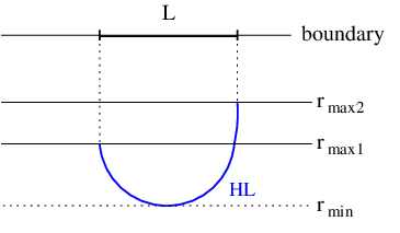
Let us first consider the single-flavor case. From the Lagrangian (61), we find the relation

e^{\Phi/2}{1\over\sqrt{(r/R)^{4}A^{2}(r)+(dr/d{\sigma})^{2}}}\left({r\over R}\right)^{4}A^{3}(r)=h\ ,

(62)

where $h$ denotes a constant of motion. Here we need to introduce two parameters, $r_{min}$ and $r_{max}$ : $r_{min}$ is determined by $\partial_{{\sigma}}r|_{r_{min}}=0$ and defines the bottom of the deformed U-shaped string, while $r_{max}$ is given by the position of the D7 brane, the endpoints of the string. Replacing $h$ by $r_{min}$ by using the relation $h=e^{\Phi/2}\left({r\over R}\right)^{2}A^{2}(r)|_{r_{min}}$ , we determine the energy $E$ and the spatial distance $L$ between the quark and anti-quark from

	$\displaystyle L=2R^{2}\int_{r_{min}}^{r_{max}}dr~I_{L},\quad E={1\over\pi\alpha^{\prime}}\int_{r_{min}}^{r_{max}}dr~I_{E}\,,$		(63)
	$\displaystyle I_{E}={A(r)e^{\Phi(r)/2}\over\sqrt{1-e^{\Phi(r_{min})}r_{min}^{4}A(r_{min})^{4}/\left(e^{\Phi(r)}r^{4}A(r)^{4}\right)}}\,,$		(64)
	$\displaystyle I_{L}={1\over r^{2}A(r)\sqrt{e^{\Phi(r)}r^{4}A(r)^{4}/\left(e^{\Phi(r_{min})}r_{min}^{4}A(r_{min})^{4}\right)-1}}\,,$		(65)

where $r_{min}$ is restricted as $0<r_{min}<r_{max}$ .

For the two-flavor case, $L$ and $E$ are given by

	$\displaystyle L=R^{2}\left(\int_{r_{min}}^{r_{max1}}dr~I_{L}+\int_{r_{min}}^{r_{max2}}dr~I_{L}\right)\,,$		(66)
	$\displaystyle E={1\over 2\pi\alpha^{\prime}}\left(\int_{r_{min}}^{r_{max1}}dr~I_{E}+\int_{r_{min}}^{r_{max2}}dr~I_{E}\right)\,,$		(67)

where $r_{max1}$ and $r_{max2}$ denote the positions of the light and heavy quark branes, respectively. They are equivalent to $w_{1}$ and $w_{2}$ for the supersymmetric case.

For the supersymmetric background, numerical plots of the energy $E(L)$ are shown in Fig. 7a. Curve (A) is a plot of $E(L)$ for heavy-light mesons, while (B) and (C) correspond to those of the light-light and heavy-heavy mesons, respectively. The curves (B) and (C) end at $(L,E)=(0,0)$ ; the energy is zero for vanishing quark-anti-quark distance, $E(0)=0$ . However, as mentioned above, in the heavy-light case the energy remains finite, even for $L=0$ .

For $L=0$ the string in Fig. 7b stretched between the D7 branes at $r_{max1}$ and $r_{max2}$ becomes just a straight line perpendicular to the boundary. Then, in the Nambu-Goto Lagrangian (61), we write $d\sigma=dr/r^{\prime}$ and take $r^{\prime}\equiv\partial r/\partial\sigma\rightarrow\infty$ . In the supersymmetric case with $q=0$ we have $A(r)=1$ , $\Phi(r)=0$ . Thus, from (61) we get

\displaystyle E(L=0)

\displaystyle={1\over 2\pi\alpha^{\prime}}\int dr\frac{1}{r^{\prime}}\sqrt{r^{\prime}{}^{2}+\left({r\over R}\right)^{4}}\stackrel{{\scriptstyle r^{\prime}\rightarrow\infty}}{{=}}\frac{1}{2\pi\alpha^{\prime}}\,\int_{r_{max1}}^{r_{max2}}\!dr\,=m_{H}-m_{L}\,.

(68)

This agrees with the meson mass result (49).

Note that the ordinary QCD string associated with the flux tube in between the quark anti-quark pair can be thought of as a projection of the Wilson loop on the boundary of the (asymptotic) AdS background, see Fig. 7b. The Wilson line for $L=0$ is aligned along the $r$ -direction and therefore projected to a point on the boundary.

6 Conclusion

We have investigated heavy-light mesons in a holographic set-up by considering the non-Abelian Dirac-Born-Infeld action for two D7 brane probes embedded at different positions. The embedding matrix is chosen to be diagonal, whereas the heavy-light mesons arise from the off-diagonal elements of the fluctuation matrix.

We considered both supersymmetric and non-supersymmetric backgrounds and found that the dominant contribution to the heavy-light meson mass is ${\cal O}(1)$ in the ’t Hooft coupling $\lambda$ , whereas for the heavy-heavy and light-light mesons it is ${\cal O}(1/\sqrt{\lambda})$ . Although this result is unexpected from the point of view of QCD, it is consistent with our Wilson loop calculation for the heavy-light mesons, as well as with the effective field theory holographic approach to heavy-light mesons of [32] which uses the Polyakov string action. As discussed in section 4.2, the ${\cal O}(1)$ contribution to the HL masses is proportional to the minimal energy of a string stretching in between two branes. In the non-supersymmetric case, the minimum energy corresponds to a string located close to the singularity (i.e. at $\rho=0$ in Fig. 4). At large ’t Hooft coupling this energy is much smaller than $m_{H}-m_{L}$ .

As far as the spectrum of heavy-light mesons is concerned, we found that the HL spectrum lies below the HH spectrum for intermediate values of the ’t Hooft coupling, $1\leq\lambda\lesssim 50$ . At larger ’t Hooft couplings, the HL meson masses exceed those of the HH mesons, which would be in conflict with phenomenology. Our results are consistent with scenarios in which QCD develops an infrared fixed point rather than a singularity, see e.g. [39] and references therein. In this case, agreement with phenomenology would be achieved, if the gauge coupling $\alpha_{s}(Q^{2})$ were of order 1 or less at the fixed point (which corresponds to $\lambda=4\pi\alpha_{s}(Q^{2})N_{c}\approx 30$ ).

A new element of our approach as compared to [32] is that it allows to distinguish scalar from vector mesons. This opens up the possibility to study the heavy quark spin effect suppression known from QCD. We see the degeneracy of scalar and vector masses for large heavy quark mass in the ${\cal N}=1$ supersymmetric scenario. It will be interesting to study the non-supersymmetric case in the future.

We conclude with some remarks on the range of validity of our approach of using the non-Abelian DBI action for two separated branes. Generally one may expect that the DBI is valid for branes separated at most by the string length $l_{s}$ . Here, however, our branes are separated by a larger distance if $m_{H}>1$ in our units of setting the string tension to one. Nevertheless our use of the non-Abelian DBI is justified by the fact that we obtain agreement with the classical string calculation of [32], as well as with the semiclassical Wilson loop analysis of a string stretching between the two branes performed in section 5 above in the present paper. Thus the classical analysis at larger length scales dominates over quantum fluctuations at shorter scales. This is at least in part due to the supersymmetry of the problem. We also note that restricting to heavy quark masses of order ${\cal O(1)}$ in the string tension will not affect the unusual $\lambda$ dependence, which intrinsically reflects the strong coupling behaviour. Physical quark masses correspond to $m_{H}\ll 1$ . In this regime, the term $m_{H}-m_{L}$ causing the unusual $\lambda$ dependence is negligible. Moreover, for the non-supersymmetric approach it should be noted that the fact that the branes approach each other in the deep interior will not alter the $\lambda$ dependence either, since all values of the coordinate $\rho$ contribute to the action. This is again in agreement with the results of [32].

Acknowledgments

K. G. would like to thank M. Tachibana and Y. Kim for discussions at an early stage of this work. J. E. would like to thank Nick Evans and Dam Son for discussions and comments. I. K. is grateful to Alejandro Daleo for a discussion. The research of I. K. is partially supported by the Swiss National Science Foundation and the Marie Curie network ‘Constituents, Fundamental Forces and Symmetries of the Universe’ (MRTN-CT-2004-005104).

References

[1] J. M. Maldacena, Adv. Theor. Math. Phys. 2, 231 (1998) [arXiv: hep-th/9711200]. S. S. Gubser, I. R. Klebanov and A. M. Polyakov, Phys. Lett. B 428, 105 (1998) [arXiv:hep-th/9802109]. E. Witten, Adv. Theor. Math. Phys. 2, 253 (1998) [arXiv:hep-th/9802150]. A.M. Polyakov, Int. J. Mod. Phys. A14, 645 (1999) [arXiv:hep-th/9809057].
[2] A. Karch and E. Katz, JHEP 0206, 043 (2002) [arXiv:hep-th/0205236].
[3] M. Kruczenski, D. Mateos, R. C. Myers and D. J. Winters, JHEP 0307, 049 (2003) [arXiv:hep-th/0304032].
[4] M. Kruczenski, D. Mateos, R. C. Myers and D. J. Winters, JHEP 0405, 041 (2004) [arXiv:hep-th/0311270].
[5] J. Babington, J. Erdmenger, N. J. Evans, Z. Guralnik and I. Kirsch, Phys. Rev. D 69, 066007 (2004) [arXiv:hep-th/0306018].
[6] N. J. Evans and J. P. Shock, Phys. Rev. D 70, 046002 (2004) [arXiv: hep-th/0403279].
[7] T. Sakai and J. Sonnenschein, JHEP 0309, 047 (2003) [arXiv:hep-th/0305049].
[8] C. Nú $\tilde{\rm n}$ ez, A. Paredes and A. V. Ramallo, JHEP 0312, 024 (2003) [arXiv: hep-th/0311201].
[9] T. Sakai and S. Sugimoto, Prog. Theor. Phys. 113, 843 (2005) [arXiv: hep-th/0412141]; T. Sakai and S. Sugimoto, Prog. Theor. Phys. 114, 1083 (2006) [arXiv:hep-th/0507073].
[10] K. Ghoroku and M. Yahiro, Phys. Lett. B 604, 235 (2004) [arXiv: hep-th/0408040].
[11] E. Antonyan, J. A. Harvey and D. Kutasov, arXiv:hep-th/0608177.
[12] K. Ghoroku, T. Sakaguchi, N. Uekusa and M. Yahiro, Phys. Rev. D 71, 106002 (2005) [arXiv:hep-th/0502088].
[13] R. Apreda, J. Erdmenger, D. Lüst and C. Sieg, JHEP 0701, 079 (2007) [arXiv: hep-th/0610276].
[14] I. Kirsch and D. Vaman, Phys. Rev. D 72, 026007 (2005) [arXiv: hep-th/0505164].
[15] J. Erdmenger and I. Kirsch, JHEP 0412, 025 (2004) [arXiv:hep-th/0408113].
[16] H. Forkel, M. Beyer and T. Frederico, arXiv:0705.1857 [hep-ph].
[17] T. Hambye, B. Hassanain, J. March-Russell and M. Schvellinger, arXiv: hep-ph/0612010.
[18] N. Evans and E. Threlfall, arXiv:0706.3285 [hep-th].
[19] L. Y. Glozman and A. V. Nefediev, arXiv:0704.2673 [hep-ph].
[20] V. G. Filev, arXiv:0706.3811 [hep-th].
[21] I. Kirsch, JHEP 0609, 052 (2006) [arXiv:hep-th/0607205].
[22] R. Heise and H. G. Svendsen, arXiv:0706.2253v1 [hep-th].
[23] H. Hata, T. Sakai, S. Sugimoto and S. Yamato, arXiv:hep-th/0701280.
[24] Z. Guralnik, S. Kovacs and B. Kulik, JHEP 0503, 063 (2005) [arXiv: hep-th/0405127].
[25] J. Erdmenger, J. Grosse and Z. Guralnik, JHEP 0506, 052 (2005) [arXiv: hep-th/0502224].
[26] D. Arean, A. V. Ramallo and D. Rodriguez-Gomez, arXiv:hep-th/0703094.
[27] K. Peeters, J. Sonnenschein and M. Zamaklar, JHEP 0602 (2006) 009 [arXiv:hep-th/0511044].
[28] A. L. Cotrone, L. Martucci and W. Troost, Phys. Rev. Lett. 96 (2006) 141601 [arXiv:hep-th/0511045].
[29] F. Bigazzi and A. L. Cotrone, JHEP 0611 (2006) 066 [arXiv:hep-th/0606059].
[30] A. Paredes and P. Talavera, Nucl. Phys. B 713, 438 (2005) [arXiv: hep-th/0412260].
[31] M. Bando, A. Sugamoto and S. Terunuma, Prog. Theor. Phys. 115, 1111 (2006) [arXiv:hep-ph/0602203].
[32] J. Erdmenger, N. Evans and J. Grosse, JHEP 0701, 098 (2007) [arXiv:hep- th/0605241].
[33] R. C. Myers, JHEP 9912, 022 (1999) [arXiv:hep-th/9910053].
[34] H. Liu and A. A. Tseytlin, Nucl. Phys. B 553 (1999) 231 [arXiv: hep-th/9903091].
[35] A. A. Tseytlin, Nucl. Phys. B 501, 41 (1997) [arXiv:hep-th/9701125].
[36] C. G. Callan and J. M. Maldacena, Nucl. Phys. B 513, 198 (1998) [arXiv:hep-th/9708147]; G. W. Gibbons, Nucl. Phys. B 514, 603 (1998) [arXiv:hep-th/9709027].
[37] I. Brevik, K. Ghoroku and A. Nakamura, Int. J. Mod. Phys. D 15, 57 (2006) [arXiv:hep-th/0505057].
[38] K. Ghoroku, M. Ishihara and A. Nakamura, Phys. Rev. D 74, 124020 (2006) [arXiv:hep-th/0609152].
[39] S. J. Brodsky, C. R. Ji, A. Pang and D. G. Robertson, Phys. Rev. D 57, 245 (1998) [arXiv:hep-ph/9705221]; S. J. Brodsky, arXiv:hep-ph/0408069.

$\displaystyle{\cal L}_{\phi^{8}}^{(2)}$	$\displaystyle={1\over 4}\partial_{r^{2}}\bar{F}\|_{w_{1}}\left((\phi^{8}_{+})^{2}+(\phi^{8}_{1})^{2}+(\phi^{8}_{2})^{2}\right)+{1\over 4}\partial_{r^{2}}\bar{F}\|_{w_{2}}\left((\phi^{8}_{-})^{2}+(\phi^{8}_{1})^{2}+(\phi^{8}_{2})^{2}\right)$
	$\displaystyle\quad+{1\over 8}(\bar{F}~G_{88}\bar{a}^{rs})\|_{w_{1}}\partial_{r}\phi^{8}_{+}\partial_{s}\phi^{8}_{+}+{1\over 8}(\bar{F}~G_{88}\bar{a}^{rs})\|_{w_{2}}\partial_{r}\phi^{8}_{-}\partial_{s}\phi^{8}_{-}$
	$\displaystyle\quad+{1\over 8}\left((\bar{F}~G_{88}\bar{a}^{rs})\|_{w_{1}}+(\bar{F}~G_{88}\bar{a}^{rs})\|_{w_{2}}\right)\left(\partial_{r}\phi^{8}_{1}\partial_{s}\phi^{8}_{1}+\partial_{r}\phi^{8}_{2}\partial_{s}\phi^{8}_{2}\right)$
	$\displaystyle\quad-{v^{2}\over 8}\left((\bar{F}~G_{88}G_{99})\|_{w_{1}}+(\bar{F}~G_{88}G_{99})\|_{w_{2}}\right)\left((\phi^{8}_{1})^{2}+(\phi^{8}_{2})^{2}\right)\,,$	(33)

$\displaystyle{\cal L}_{\tilde{A}}^{(2)}$	$\displaystyle={1\over 4}(\bar{F}\bar{a}^{rp}\bar{a}^{sq})\|_{w_{1}}\tilde{F}_{rs}^{+}\tilde{F}_{pq}^{+}+{1\over 4}(\bar{F}\bar{a}^{rp}\bar{a}^{sq})\|_{w_{2}}\tilde{F}_{rs}^{-}\tilde{F}_{pq}^{-}$
	$\displaystyle\quad+{1\over 4}\left((\bar{F}\bar{a}^{rp}\bar{a}^{sq})\|_{w_{1}}+(\bar{F}\bar{a}^{rp}\bar{a}^{sq})\|_{w_{2}}\right)\left(\tilde{F}_{rs}^{1}\tilde{F}_{pq}^{1}+\tilde{F}_{rs}^{2}\tilde{F}_{pq}^{2}\right)$
	$\displaystyle\quad+{v^{2}\over 8}\left((\bar{F}~G_{99}\bar{a}^{rs})\|_{w_{1}}+(\bar{F}~G_{99}\bar{a}^{rs})\|_{w_{2}}\right)\left(\tilde{A}_{r}^{1}\tilde{A}_{s}^{1}+\tilde{A}_{r}^{2}\tilde{A}_{s}^{2}\right)\,,$	(41)