A Linearization of Connes’ Embedding ProblemThanks: †Research supported in part by NSERC grant RGPIN/341303-2007Thanks: ∗Research supported in part by NSF grant DMS-0600814
Abstract.
We show that Connes’ embedding problem for II1–factors is equivalent to a statement about distributions of sums of self–adjoint operators with matrix coefficients. This is an application of a linearization result for finite von Neumann algebras, which is proved using asymptotic second order freeness of Gaussian random matrices.
2000 Mathematics Subject Classification
46L10,15A421. Introduction
A von Neuman algebra is said to be finite if it possesses a normal, faithful, tracial state . By “finite von Neumann algebra” , we will always mean such an algebra equipped with a fixed such trace . Connes’ embedding problem asks whether every such with a separable predual can be embedded in an ultrapower of the hyperfinite II1–factor in a trace–preserving way. This is well known to be equivalent to the question of whether a generating set for has microstates, namely, whether there exist matrices over the complex numbers whose mixed moments up to an arbitrary given order approximate those of the elements of with respect to , to within an arbitrary given tolerance. (See section 3 where precise definitions and, for completeness, a proof of this equivalence are given.) We will say that posseses Connes’ embedding property if it embeds in . (It is known that possession of this property does not depend on the choice of faithful trace .)
Seen like this, Connes’ embedding probem, which is open, is about a fundamental approximation property for finite von Neumann algebras. There are several important results, due to E. Kirchberg [13], F. Rădulescu [18], [19], [20], [21] and N. Brown [5], that have direct bearing on this problem; see also G. Pisier’s paper [17] and N. Ozawa’s survey [16].
Recently, H. Bercovici and W.S. Li [4] have proved a property enjoyed by elements in a finite von Neumann algebra that embeds in . This property is related to a fundamental question about spectra of sums of operators: given Hermitian matrices or, more generally, Hermitian operators and with specified spectra, what can the spectrum of be? For matrices, a description was conjectured by Horn [11] and was eventually proved to be true by work of Klyachko, Totaro, Knutson, Tao and others, if by “spectrum” we mean the eigenvalue sequence, namely, the list of eigenvalues repeated according to multiplicity and in non–increasing order. In this description, the possible spectrum of is a convex subset of described by certain inequalities, called the Horn inequalities. See Fulton’s exposition [8] or, for a very abbreviated decription, section 4 of this paper. We will call this convex set the Horn body associated to and , and denote it by , where and are the eigenvalue sequences of and , respectively.
Bercovici and Li [3], [4] have studied the analogous question for and self–adjoint elements of a finite von Neumann algebra , namely: if spectral data of and of are specified, what are the possible spectral data of ? Here, by “spectral data” one can take the distribution (i.e., trace of spectral measure) of the operator in question, which is a compactly supported Borel probability measure on , or, in a description that is equivalent, the eigenvalue function of the operator, which is a nonincreasing, right–continuous function on that is the non–discrete version of the eigenvalue sequence.
In [4], for given eigenvalue functions and , they construct a convex set, which we will call , of eigenvalue functions. This set can be viewed as a limit (in the appropriate sense) of Horn bodies as . They show that the eigenvalue function of must lie in whenever and lie in and have eigenvalue functions and, respectively, .
Bercovici and Li’s result provides a concrete method to attempt to show that a finite von Neumann algebra does not embed in : find self–adjoint and in for which one knows enough about the spectral data of , and , and find a Horn inequality (or, rather, it’s appropriate modification to the setting of eigenvalue functions) that is violated by these.
Their result also inspires two further questions:
Question 1.1.
- (i)
Which Horn inequalitites must be satisfied by the spectral data of self–adjoints , and in arbitrary finite von Neumann algebras?
- (ii)
(conversely to Bercovici and Li’s result): If we know, for all self–adjoints and in an arbitrary finite von Neumann algebra , calling their eigenvalue functions and , respectively, that the eigenvalue function of belongs to , is this equivalent to a positive answer for Connes’ embedding problem?
Question (ii) above is easily seen to be equivalent to the same question, but where and are assumed to lie in some copies of the matrix algebra in , for some .
Bercovici and Li, in [3], partially answered the first question by showing that a subset of the Horn inequalities (namely, the Freede–Thompson inequalities) are always satisfied in arbitrary finite von Neuman algebras.
We attempted to address the second question. We are not able to answer it, but we prove a related result (Theorem 4.6) which answers the analogous question for what we call the quantum Horn bodies. These are the like the Horn bodies, but with matrix coefficients. More precisely, if and are nonincreasing real sequences of length and if and are self–adjoint matrices for some , then the quantum Horn body is the set of all possible eigenvalue functions of matrices of the form
| (1) |
as and range over the unitaries. (In fact, Theorem 4.6 concerns the appropriate union of such bodies over all — see section 4 for details.)
Our proof of Theorem 4.6 is an application of a linearization result (Theorem 2.1) in finite von Neumann algebras, which implies that if , , and are self–adjoint elements of a finite von Neuman algebra and if the distributions (i.e., the moments) of
| (2) |
and
| (3) |
agree for all and all self–adjoint , then the mixed moments of the pair agree with the mixed moments of the pair , i.e. the trace of
| (4) |
agrees with the trace of.
| (5) |
for all and all . This is equivalent to there being a trace–preserving isomorphism from the von Neumann algebra generated by and onto the von Neumann algebra generated by and , that sends to .
This linearization result for von Neumann algebras is quite analogous to one for C∗–algebras proved by U. Haagerup and S. Thorbjørnsen [10] (and quoted below as Theorem 2.2). However, our proof of Theorem 2.1 is quite different from that of Haagerup and Thorbjørnsen’s result. Our linearization result is not so surprising because, for example, for a proof it would suffice to show that the trace of an arbitrary word of the form (4) is a linear combination of moments of various elements of the form (2). One could imagine that a combinatorial proof by explicit choice of some and , etc., may be possible. However, our proof does not yield an explicit choice. Rather, it makes a random choice of and . For this we make crucial use of J. Mingo and R. Speicher’s results on second order freeness of independent GUE random matrices.
Finally, we need more than just the linearization result. We use some ultrapower techniques to reverse quantifiers. In particular, we show that for the von Neumann algebra generated by and to be embeddable in , it suffices that for all self–adjoint matrices and , there exists and lying in such that the distributions of (2) and (3) agree. For this, it is for technical reasons necessary to strengten the linearization result (Theorem 2.1) by restricting the matrices and to have spectra in a nontrivial bounded interval .
To recap: in Section 2 we prove the linearization result, making use of second order freeness. In Section 3, we review Connes’ embedding problem and it’s formulation in terms of microstates; then we make an ultrapower argument to prove a result (Theorem 3.4) characterizing embeddability of a von Neumann algebra generated by self–adjoints and in terms of distributions of elements of the form (2). In Section 4, we describe the quantum Horn bodies, state some related questions and consider some examples. We finish by rephrasing Connes’ embedding problem in terms of the quantum Horn bodies.
2. Linearization
Notation: we let denote the set of complex matrices, while means the set of self–adjoint elements of . We denote by the unnormalized trace, and we let be the normalized trace (sending the identity element to ).
The main theorem of this section is
Theorem 2.1.
Let be a von Neumann algebra generated by selfadjoint elements and be a von Neumann algebra generated by selfadjoint elements . Let be a faithful trace on and be a faithful trace on .
Let be real numbers and suppose that for all and all in whose spectra are contained in the interval , the distributions of and are the same.
Then there exists an isomorphism such that and .
The statement of this theorem can be thought of as a version for finite von Neumann algebras of the following –algebra linearization result of Haagerup and Thorbjørnsen.
Theorem 2.2 ([10]).
Let (respectively ) be a unital –algebra generated by selfadjoints (resp. ) such that for all positive integers and for all ,
| (6) |
and
| (7) |
have the same spectrum, then there exists an isomorphism from onto such that .
However, our proof of Theorem 2.1 is quite different from the proof of Theorem 2.2. In addition, there is the notable difference that we do not need to consider matrix coefficients of the identity. In order to simplify our notation, we restrict to proving the case of Theorem 2.1. We indicate at Remark 2.10 how our proof works in general.
Let be the free monoid generated by free elements , and
| (8) |
be the free unital –algebra over selfadjoint elements .
Let be the rotation action of the integers on the set , given by
| (9) |
Let denote the set of orbits of this action. Let be the vector space spanned by the commutators with . Recall that an (algebraic) trace is a linear map such that . Equivalently, a linear map is a trace if and only if it vanishes on .
Lemma 2.3.
For any orbit , let . Then splits as the direct sum
| (10) |
Moreover, the commutator subspace splits accross this direct sum as
| (11) |
Furthermore, is of codimension in and we have
| (12) |
Proof.
The direct sum decomposition (10) is obvious. From the relation
| (13) |
one easily sees
| (14) | |||
| (15) |
from which the assertions follow. ∎
An orbit is a singleton if and only if it is of the form for some and some integer . For each orbit that is not a singleton, choose a representative of the orbit of the form
| (16) |
with and , and collect them together in a set , of representatives for all the orbits in that are not singletons.
Let and () be two families of polynomials, which we will specify later on, such that the degree of each and is . For written as in (16), we let
| (17) |
Lemma 2.4.
The family
| (18) |
is linearly independent and spans a space such that
| (19) | ||||
| (20) |
Proof.
For an orbit , the total degree of all agree; denote this integer by . Letting and using Lemma 2.3, an argument by induction on shows . This implies (19).
To see the linear independece of (18) and to see (20), suppose
| (21) |
for complex numbers , and , not all zero, and let us show . We also write
| (22) |
for complex numbers .
Suppose for some and let be of largest degree such that . Let be the orbit of . Then
| (23) |
By the direct sum decomposition (11), we get .
On the other hand, if for some and some . Suppose is the largest such that . Then , and .
Finally, if for all and if for some and some , then we are left with and . ∎
We recall that a Gaussian unitary ensemble (also denoted by GUE) is the probability distribution of the random matrix on , where has independent complex gaussian entries of variance . This distribution has a density proportional to with respect to the Lebesgue measure on the selfadjoint real matrices. A classical result of Wigner [24] states that the empirical eigenvalue distribution of a GUE converges as in moments to Wigner’s semi–circle distribution
| (24) |
If we view the for various as matrix–valued random variables over a commone probability space, then almost surely, the largest and smallest eigenvalues of converge as to , respectively. This was proved by Bai and Yin [2] (see also [1]). See [9] for further discussion and an alternative proof.
We recall that the Chebyshev polynomials of the first kind are the monic polynomials orthogonal with respect to the weight . Alternatively, they are determined by their generating series
| (25) |
Similarly, Chebyshev polynomial of the second kind are orthogonal with respect to the weight and have the generating series
| (26) |
The following result is random matrix folklore, but it is implied by more general results of Johansson ([12], Cor 2.8):
Proposition 2.5.
Let be the GUE of dimension and the Chebyshev polynomial of second kind. Let
| (27) |
Then for every , the real random vector
| (28) |
tends in distribution as toward a vector of independent standard real Gaussian variables.
Consider two GUE random matrix ensembles and , that are independent from each other (for each ). Voiculescu proved [22] that these converge in moments to free semicircular elements and having first moment zero and second moment , meaning that we have
| (29) |
for all and , (where is a trace with respect to which and are semicircular and free). Of course, by freeness, this implies that if and are polynomials such that for all , then
| (30) |
Mingo and Speicher [15] have proved some remarkable results about the related fluctuations, namely, the (magnified) random variables (31) below. These are asymptotically Gaussian and provide examples of the phenomenon of second order freeness, which has been treated in a recent series of papers [15], [14], [6]. In particular, the following theorem is a straightforward consequence of some of the results in [15].
Theorem 2.6.
Let and be independent GUE random matrix ensembles. Let be a –semicircular element with respect to a trace . Let and let be polynomials with real coefficients such that for each . Then the random variable
| (31) |
converges in moments as to a Gaussian random variable. Moreover, if and if are real polynomials such that for each , then
| (32) | ||||
| (33) | ||||
| (34) |
where the subscripts of and are taken modulo . Furthermore, for any polynomial , we have
| (35) | ||||
| (36) |
If is any unital algebra and if , we let
| (37) |
be the algebra homomorphism given by
| (38) |
In the corollary below, which follows directly from Theorem 2.6 and Proposition 2.5, we take as the algebra of random matrices (over a fixed probability space) whose entries have moments of all orders.
Corollary 2.7.
Let and be real numbers with . Let be independent copies of
| (39) |
where is distributed as the GUE of dimension . Let
| (40) |
and
| (41) |
If , then we have
| (42) |
and we let . If for and , then we have
| (43) |
where is as in (27), and we set .
Then the random variables
| (44) |
where is as in Lemma 2.4, converge in moments as to independent, non–trivial, centered, Gaussian variables.
The following lemma is elementary and we will only use it in the especially simple case of . We will use it to see that for a sequence of random variables converging in moments to a nonzero random variable, we have that is bounded away from zero as . This is all unsurprising and well known, but we include proofs for completeness.
Lemma 2.8.
Let be a random variable with finite first and second moments, denoted and . Suppose and . Then for every satisfying
| (45) |
there is , a continuous function of , and , such that and
| (46) |
More precisely, we may choose
| (47) |
Proof.
Say that is a random variable on a probability space and let be the set where takes values . Using the Cauchy–Schwarz inequality, we get
| (48) |
which yields
| (49) |
If , then this gives . When , consider the polynomial
| (50) |
It’s minimum value occurs at and we have (by the Cauchy–Schwarz inequality) and . Therefore, letting denote the larger of the roots of , we have . Moreover, if and , then . Taking , we conclude that , and we have the formula (47). It is easy to see that is a continuous function of , and . ∎
Lemma 2.9.
Let be real numbers. For matrices and , consider the maps . Then we have
| (51) |
Proof.
The inclusion in (51) follows from the trace property.
Let and make the choice of polynomials and described in Corollary 2.7. Letting and be as in Lemm 2.4, for each , we will find matrices and such that
| (52) |
By (19) and (20) of Lemma 2.4, this will suffice to show in (51). Rather than find and explicitly, we make use of random matrices.
We may write
| (53) |
with , and , not all zero. If is the only nonzero coefficient, then is a nonzero constant multiple of the identity and any choice of and gives (52). So assume some or . Let and be the independent random matrices as described in Corollary 2.7. Extend the function that was defined in Corollary 2.7 to a function by linearity and by setting . By that corollary, the random variable
| (54) |
converges as in moments to a Gausian random variable with some nonzero variance . It is now straightforward to see that
| (55) |
is bounded away from zero as . Indeed, If , then since and since the second moment of stays bounded as , the quantity (55) stays bounded away from zero as . On the other hand, if , then considering the second and fourth moments of and applying Lemma 2.8, we find such that for all sufficiently large, we have . Thus, also in this case, the quantity (55) is bounded away from zero as .
Proof of Theorem 2.1.
As mentioned before, we concentrate on the case , and the other cases follow similarly. By the Gelfand–Naimark–Segal representation theorem, it is enough to prove that for all monomials in non–commuting variables, we have
| (57) |
Rephrased, this amounts to showing that we have
| (58) |
for all . By hypothesis, for all , all and all we have
| (59) |
Developing the right–hand–side minus the left–hand–side of (59) gives that the equality
| (60) |
holds true for any choice . This equation can be rewritten as
| (61) |
where is a set representatives, one from each orbit in , of the monomials of degree , and where is the cardinality of each class.
Remark 2.10.
We only proved the result for . The proof for arbitrary is actually exactly the same. The only difference is that the notations in the definition of second order freeness is more cumbersome, but Theorem 2.6 as well as the other lemmas are unchanged.
Remark 2.11.
The main ingredient in the proof of Theorem 2.1 is to provide a method of constructing such that
| (63) |
whenever this is not ruled out by reasons of symmetry. Our approach is probabilistic, and makes unexpected use of second–order freeness. In particular, our approach is non–constructive. It would be interesting to find a direct approach.
It is natural to wonder how much one can shrink the choice of matrices from which and in Remark 2.11 are drawn. We would like to point out here that in Lemma 2.9 we needs at least infinitely many values of . More precisely, we can prove the following:
Proposition 2.12.
For each , we have
| (64) |
Proof.
Without loss of generality (for example, by taking ), it will be enough to prove
| (65) |
for each .
Following the proof of Theorem 2.1, let be the degree vector subspace of the quotient of vector spaces . The dimension of is at least .
Consider the commutative polynomial algebra in the variables . Consider matrices
| (66) |
over this ring. In this setting,
| (67) |
is a -linear map from to that vanishes on and every map of the form for is composed with some evaluation map on the polynomial ring . Therefore, we have
| (68) |
We denote also by the induced map
| (69) |
Clearly, maps into the vector space of homogeneous polynomials in of degree . The space of homogenous polynomials of degree in variables has dimension equal to the binomial coefficient . Therefore, there exists a constant , depending on , such that maps into a subspace of complex dimension . For fixed , there is large enough so that one has . Therefore, by the rank theorem, the kernel of restricted to must be non–empty. Combined with (68), this proves (65). ∎
3. Application to embeddability
We begin by recalling the ultrapower construction. Let denote the hyperfinite II1–factor and its normalized trace. Let be a free ultrafilter on and let denote the ideal of consisting of those sequences such that . Then is the quotient , which is actually a von Neumann algebra.
Let be a von Neumann algebra with normal, faithful, tracial state .
Definition 3.1.
The von Neumann algebra is said to have Connes’ embedding property if can be embedded into an ultra power of the hyperfinite von Neumann algebra in a trace–preserving way.
Definition 3.2.
If is a finite subset of , we say that has matricial microstates if for every and every , there is and there are self–adjoint matrices such that whenever and , we have
| (70) |
where is the normalized trace on .
It is not difficult to see that if has matricial microstates, then for every and , there is such that for every there are matrices whose mixed moments approximate those of in the sense specified above. Also, as proved by an argument of Voiculescu [23], if has matricial microstates, then each approximating matrix above can be chosen to have norm no greater than .
The following result is well known. For future reference, we briefly describe a proof.
Proposition 3.3.
Let be a von Neumann algebra with seperable predual and a normal, faithful, tracial state on . Then the following are equivalent:
- (i)
has Connes’ embedding property.
- (ii)
Every finite subset has matricial microstates.
- (iii)
If is a generating set for , then every finite subset of has matricial microstates.
In particular, if is a finite generating set of then the above conditions are equivalent to having matricial microstates.
Proof.
The implication (i)(ii) follows because if , then choosing any representatives of the in , we find elements of whose mixed moments up to order approximate those of the as closely as desired. Now we use that any finite subset of is approximately (in –norm) contained in some copy , for some sufficiently large.
The implication (ii)(iii) is evident.
For (iii)(i), we may without loss of generality suppose that for some sequence possibly with repetitions. Fix , let and let be matricial microstates for so that (70) holds for all and for , and assume for all . Choose a unital –homomorphism , and let . Let , where we set if . Let be the image of in . Then has the same joint distribution as , and this yields an embedding sending to . ∎
A direct consequence of Theorem 2.1 is:
Theorem 3.4.
Suppose that a von Neumann algebra with trace is generated by self–adjoint elements and . Let be real numbers. Then has Connes’ embedding property if and only if there exists such that for all whose spectra are contained in ,
| (71) |
In this section we will prove that Connes’ embedding property is equivalent to a weaker condition.
Lemma 3.5.
Suppose that a von Neumann algebra with trace is generated by self–adjoint elements and . Let be real numbers and for every , let be a dense subset of the set of all elements of whose spectra are contained in the interval . Then has Connes’ embedding property if and only if for all finite sets and all choices of and , , there exists such that
| (72) | |||
| (73) | |||
| (74) |
Proof.
Necessity is clear.
For sufficiency, we’ll use an ultraproduct argument. Let be an enumeration of a countable, dense subset of the disjoint union . We let be such that . For each , let be elements of satisfying and
| (75) |
for all . In particular, for and all . Let
| (76) |
be such that and the image of in is (). This implies that for all and all , we have
| (77) |
which in turn implies that there is a set belonging to the ultrafilter such that for all and all , we have
| (78) |
For , let and for , let
| (79) |
Then for all , we have
| (80) |
Let be the image in of . Then we have
| (81) |
for all . By density, we have that (71) holds for all and all having spectra in . Therefore, by Theorem 3.4, is embeddable in . ∎
Theorem 3.6.
Suppose that a von Neumann algebra with trace is generated by self–adjoint elements and and suppose that both and are positive and invertible. Then has Connes’ embedding property if and only if for all and all there exists such that
| (82) | |||
| (83) | |||
| (84) |
hold.
Proof.
Again, necessity is clear.
For the reverse implication, we will show that the conditions of Lemma 3.5 are satisfied. Suppose that for all and all , there exist and such that (82)–(84) hold. Let be such that
| (85) |
Let be the set of all elements of having spectra in the interval . We will show that the condition appearing in Lemma 3.5 is satisfied for these sets. Let and for every let , and . We will find such that (72)–(74) hold. For any and , the spectrum of lies in the interval
| (86) |
Let and let be the block diagonal matrices
| (87) |
By hypothesis, there exists such that (82)–(84) hold. We have
| (88) |
and similarly for . Since the spectrum of lies in for all and , the spectrum of lies in as does the spectrum of . Since the intervals in the family are pairwise disjoint, it follows that for every , the projections
arise as the spectral projection of and, respectively, , for the inverval . Cutting by these spectral projections, we thus obtain that the distributions of and are the same, as required. ∎
4. Quantum Horn boddies
Let denote the set of –tuples of real numbers listed in nonincreasing order. The eigenvalue sequence of an self–adjoint matrix is its sequence of eigenvalues repeated according to multiplicity and in nonincreasing order, so as to lie in . Consider and in . Let be the set of all possible eigenvalue sequences of , where and are self–adjoint matrices with eigenvalue sequences and , respectively. Thus, is the set of all eigenvalue sequences of –matrices of the form
| (89) |
where is the group of –unitary matrices. Klyatchko, Totaro, Knutson and Tao described the set in terms first conjectured by Horn. See Fulton’s exposition [8]. Taking traces, clearly every must satisfy
| (90) |
Consider the inequality
| (91) |
for a triple of subsets of . Horn defined sets of triples of subsets of of the same cardinality , by the following recursive procedure. Set
| (92) |
When , set . Otherwise, let
| (93) | ||||
The result of Klyatchko, Totaro, Knutson and Tao is that consists of those elements such that the equality (90) holds and the inequality (91) holds for every triple . We will refer to as the Horn body of and . It is, thus, a closed, convex subset of .
The analogue of this situation occuring in finite von Neumann algebras has been considered by Bercovici and Li [3], [4]; let us summarize part of what they have done. We denote by the set of all right–continuous, nonincreasing, bounded functions . Let be a von Neumann algebra with normal, faithful, tracial state and let . The distribution of is the Borel measure , supported on the spectrum of , such that
| (94) |
The eigenvalue function of is defined by
| (95) |
We call the set of all eigenvalue functions. It is an affine space, where we take scalar multiples and sums of functions in the usual way. Identifying with the set of all compactly supported Borel measures on the real line, it is a subspace of the dual of . We endow with the weak∗–topology inherited from this pairing.
It is clear that for every and every II1–factor , there is such that . Note that if and if has eigenvalue sequence , then its eigenvalue function is given by
| (96) |
In this way, is embedded as a subset of , and the affine structure on inherited from corresponds to the usual one on coming from the vector space structure of .
For a set , consider the triple , where for , we set
| (97) |
Let
| (98) |
Theorem 4.1 ([4], Thm. 3.2).
For any , there exists self–adjoint elements and in the ultrapower of the hyperfinite II1–factor with , and if and only if
| (99) |
and, for every , we have
| (100) |
Given eigenvalue functions , let be the set of all such that (99) holds and (100) holds for every . Since the functions in are uniformly bounded, we see that is a compact, convex subset of .
Now we consider an alternative formulation of a special case of Theorem 4.1. Let and . For , let
| (101) |
For , this is just the set of eigenvalue functions corresponding to the Horn body . Let
| (102) |
As a consequence of Bercovici and Li’s results we have the following.
Proposition 4.2.
Let and let and be the correspoding eigenvalue functions. Then
| (103) |
is a compact, convex subset of .
If Connes’ embedding problem has a positive solution, then for every II1–factor and every whose eigenvalue functions are and , respectively, we have .
Proof.
The inclusion in (103) is clear. For the reverse inclusion, let . Then (99) holds and (100) holds for every . For , let be obtained by averaging over the intervals of length , namely,
| (104) |
Then corresponds to an eigenvalue sequence . We have
| (105) |
and, for every for , we have
| (106) |
Therefore, taking to be a multiple of , by the theorem formerly known as Horn’s conjecture, we have and, consequently, . Since converges as to , we have . This proves the equality (103).
The final statment is a consequence of Bercovici and Li’s result, Theorem 4.1. ∎
Bercovici and Li’s results provide a means of trying to find a II1–factor that lack’s Connes’ embedding property: namely, by finding self–adjoint elements such that ; this amounts to finding some such that
| (107) |
On the other hand we will use Theorem 3.6 to see that Connes’ embedding problem is equivalent to an anlogous question about versions of the Horn body with “matrix coefficients.”
Let , and . We introduce the set of the eigenvalue functions of all matrices of the form
| (108) |
Although, for reasons that will be immediately apparent, we choose to view as a subset of , we may equally well consider the corresponding eigenvalue sequences and view as a subset of . Comparing to (89), the set is seen to be the analogue of the Horn body , but with “coefficients” and . We will refer to these sets as quantum Horn bodies.
The example below shows that need not be convex, even in the case where commute.
Example 4.3.
Let
| (109) |
and let . Then the matrices of the form (108) are all unitary conjugates of the matrices
| (110) |
for . One easily finds the eigenvalues of to be
| (111) | ||||
| (112) | ||||
| (113) | ||||
| (114) |
where . Then the set is a –dimensional subset of –space that is far from being convex. For example, a plot of the projection of this set onto the last two coordinates is the curve in Figure 1.
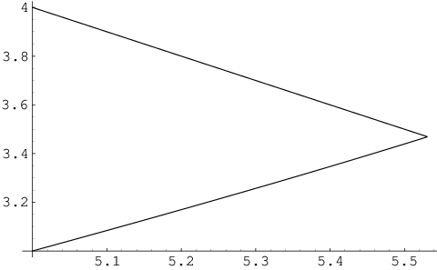
The upper part of this curve is a line segment, while the lower part is not.
Extending the notions introduced above, for integers , let be the set of the eigenvalue functions of all matrices of the form
| (115) |
If divides , then we have
| (116) |
Let us define
| (117) |
where the closure is in the weak∗–topology for described earlier in this section. Note that the set is compact.
Question 4.4.
Though Example 4.3 shows that need not be convex, is it true that must be convex, or even that must be convex for all sufficiently large? Note that it is clear that is convex with respect to the affine structure on that arises from taking convex combinations of measures, under the correspondence between and the set of Borel probability measures on . However, we are interested in the other affine structure of , resulting from addition of functions on .
For with eigenvalue sequences , we obviously have
| (118) |
and
| (119) |
The following example shows that these inclusions can be strict.
Example 4.5.
Let
| (120) |
One directly sees that for any eigenvalue sequences and of length and any , the eigenvalue sequence of
| (121) |
is the re–ordering of the concatenation of and . Thus, has only one element. Moreover, dilating to does not change the corresponding eigenvalue functions of
| (122) |
This shows that has only one element. Now we easily get
| (123) |
where means the eigenvalue sequence of , etc.
For a II1–factor, we define to be the set of all eigenvalue functions of all operators of the form
| (124) |
where and are self–adjoint elements of whose eigenvalue functions agree with those of the matrices and , respectively (see (96) for an explicit description of the latter). It is easliy seen that we have
| (125) |
Let
| (126) |
where the union is over all II1–factors with separable predual (acting on a specific separable Hilbert space, say). Using an ultraproduct argument, one can show that is closed in and compact. Also, one obviously has
| (127) |
Theorem 3.6 gives us the following equivalent formulation of the embedding question.
Theorem 4.6.
The following are equivalent:
- (i)
Every II1–factor with separable predual has Connes’ embedding property.
- (ii)
For all integers and all , and , we have
(128)
Proof.
Suppose (ii) holds. It is well known that to solve Connes’ embedding problem in the affirmative, it will suffice to show that every tracial von Neuman algebra that is generated by two self–adjoints and is embeddable in .
So suppose is generated by self–adjoints and . By Proposition 3.3, it will suffice to show that and have matricial microstates. Approximating and , if necessary, we may without loss of generality assume that the eigenvalue functions of both belong to for some , namely, that they correspond to sequences and, respectively, in . By adding constants, if necessary, we may without loss of generality assume that and are positive and invertible. Let and let . Using (125) and (128), there are such that (82)–(84) of Theorem 3.6 hold. So by that theorem, the pair has matricial microstates. ∎
References
- [1] Z.D. Bai, Methodology in spectral analysis of large dimensional random matrices, A review, Statistica Sinica 9 (1999), 611–677.
- [2] Z.D. Bai and Y.Q. Yi, Necessary and sufficient conditions for the almost sure convergence of the largest eigenvalue of a Wigner matrix, Ann. of Probab. 16 (1988), 1729–1741.
- [3] H. Bercovici and W.S. Li, Inequalities for eigenvalues of sums in a von Neumann algebra, “Recent advances in operator theory and related topics (Szeged, 1999),” Oper. Theory Adv. Appl. 127 Birkhäuser, Basel, 2001, pp. 113–126.
- [4] H. Bercovici and W.S. Li, Eigenvalue inequalities in an embeddable factor, Proc. Amer. Math. Soc. 134 (2006), 75–80.
- [5] N. Brown, Connes’ embedding problem and Lance’s WEP, Int. Math. Res. Not. 2004, 501–510.
- [6] B. Collins, J. Mingo, P. Śniady and R. Speicher, Second order freeness and fluctuations of random matrices III. Higher order freeness and free cumulants, Documenta Math. 12 (2007), 1-70.
- [7] M. De La Salle, in preparation.
- [8] W. Fulton, Eigenvalues, invariant factors, highest weights, and Schubert calculus, Bull. Amer. Math. Soc. (N.S.) 37 (2000), 209–249.
- [9] U. Haagerup and S. Thorbjornsen, Random matrices with complex Gaussian entries, Expo. Math. 21 (2003), 293–337.
- [10] U. Haagerup and S. Thorbjørnsen, A new application of random matrices: is not a group. Ann. of Math. (2) 162 (2005), no. 2, 711–775.
- [11] A. Horn, Eigenvalues of sums of Hermitian matrices, Pacific J. Math. 12 (1962), 225-241.
- [12] K. Johansson, On fluctuations of eigenvalues of random Hermitian matrices, Duke Math. J. 91 (1998), no. 1, 151–204.
- [13] E. Kirchberg, On nonsemisplit extensions, tensor products and exactness of group -algebras, Invent. Math. 112 (1993), 449–489.
- [14] J. Mingo, P. Śniady and R. Speicher, Second order freeness and fluctuations of random matrices: II. Unitary random matrices, Adv. Math. 209 (2007) 212–240.
- [15] J. Mingo and R. Speicher, Second order freeness and fluctuations of random matrices. I. Gaussian and Wishart matrices and cyclic Fock spaces, J. Funct. Anal. 235 (2006), no. 1, 226–270.
- [16] N. Ozawa, About the QWEP conjecture, Internat. J. Math. 15 (2004), 501–530.
- [17] G. Pisier, A simple proof of a theorem of Kirchberg and related results on C∗–norms, J. Operator Theory 35 (1996), 317–335.
- [18] F. Rădulescu, Convex sets associated with von Neumann algebras and Connes’ approximate embedding problem, Math. Res. Lett. 6 (1999), 229–236.
- [19] F. Rădulescu, A comparison between the max and min norms on , J. Operator Theory 51 (2004), 245–253.
- [20] F. Rădulescu, Combinatorial aspects of Connes’s embedding conjecture and asymptotic distribution of traces of products of unitaries, Operator Theory 20, Theta Ser. Adv. Math., 6, Theta, Bucharest, 2006 pp. 197–205.
- [21] F. Rădulescu, A non-commutative, analytic version of Hilbert’s 17-th problem in type II1 von Neumann algebras, preprint, arXiv:math/0404458.
- [22] D.V. Voiculescu, Limit laws for random matrices and free products, Invent. Math. 104 (1991), 201–220.
- [23] D. Voiculescu, The analogues of entropy and of Fisher’s information measure in free probability theory. II. Invent. Math. 118 (1994), 411–440.
- [24] E. Wigner, Characteristic vectors of bordered matrices with infinite dimensions, Ann. of Math. 62 (1955), 548–564.