Order from Randomness

Simple models of evolution may sometimes lead to complicated and unexpected behavior, cf. e.g. [6]. We consider the following elementary problem. Let us choose a finite set of $n$ points $\left\{p_{i}\right\}$ distributed arbitrarily (in particular randomly) on the plane. Let us further label these points in a unique but otherwise quite arbitrary way:

$$p_{0},\ p_{1},\ldots,\ p_{n-1}$$

(1)

Of course, given any set one has $n!$ different ways of labelling its elements. We can further treat these points as two-dimensional sequence of vectors attached to the origin of the Cartesian coordinates.

Define next the following ”cyclic” sequence of vector differences and denote them $p_{i}(1)$:

	$\displaystyle p_{0}(1)$	$\displaystyle=$	$\displaystyle p_{1}-p_{0}$		(2)
	$\displaystyle p_{1}(1)$	$\displaystyle=$	$\displaystyle p_{2}-p_{1}$
			$\displaystyle\cdots$
	$\displaystyle p_{n-2}(1)$	$\displaystyle=$	$\displaystyle p_{n-1}-p_{n-2}$
	$\displaystyle p_{n-1}(1)$	$\displaystyle=$	$\displaystyle p_{0}-p_{n-1}$

It represents a sequence of $n$ new vectors which, after appropriate shifting, may also be attached to the origin of coordinates. We can consider these points as the next phase of some discrete time evolution and repeat the process iteratively many times. Note that this process is strictly deterministic, that is, once chosen the initial points and their labelling, the rest of the discrete evolution is fully determined regardless of how many steps has been performed. The only chaotic element in this process is included in the initial distribution, unless this distribution is deliberately chosen as regular.

Each transition $t\rightarrow t+1$ in this discrete evolution can be written using more suggestive matrix notation as:

$$\left(\begin{array}[]{c}x_{0}(t+1)\\ x_{1}(t+1)\\ ~\vdots\\ x_{n-2}(t+1)\\ x_{n-1}(t+1)\end{array}\right)=\left(\begin{array}[]{ccccc}-1&+1&0&\cdots&0\\ 0&-1&+1&\cdots&0\\ \vdots&\vdots&\vdots&\vdots&\vdots\\ 0&0&\cdots&-1&+1\\ +1&0&\cdots&0&-1\end{array}\right)\left(\begin{array}[]{c}x_{0}(t)\\ x_{0}(t)\\ \vdots\\ x_{n-2}(t)\\ x_{n-1}(t)\end{array}\right)$$

(3)

for the $x$ coordinate and similarly for the $y$ coordinate, where $t=0,1,2,...$ Consequently, starting from the initial configuration, after $t$ evolution steps, we get:

$$\left(\begin{array}[]{c}x_{0}(t)\\ x_{1}(t)\\ \vdots\\ x_{n-2}(t)\\ x_{n-1}(t)\end{array}\right)=\left(\begin{array}[]{ccccc}-1&+1&0&\cdots&0\\ 0&-1&+1&\cdots&0\\ \vdots&\vdots&\vdots&\vdots&\vdots\\ 0&0&\cdots&-1&+1\\ +1&0&\cdots&0&-1\end{array}\right)^{{\Huge t}}\left(\begin{array}[]{c}x_{0}(0)\\ x_{0}(0)\\ \vdots\\ x_{n-2}(0)\\ x_{n-1}(0)\end{array}\right)$$

(4)

where the power is understood as matrix power, of course. (Matrix which appears in (3) and (4) is a special case of so-called circulant matrix, cf. [5], for pedagogical review see [4].)

Using different, perhaps less evocative notation, this algorithm can also be written in coordinate representation as:

	$\displaystyle x_{k}(t)$	$\displaystyle=$	$\displaystyle\left(-1\right)^{t}\sum\limits_{i=0}^{t}\left(-1\right)^{i}\binom{t}{i}x_{k+i}(0)$		(5)
	$\displaystyle y_{k}(t)$	$\displaystyle=$	$\displaystyle\left(-1\right)^{t}\sum\limits_{i=0}^{t}\left(-1\right)^{i}\binom{t}{i}y_{k+i}(0)$

Equations (5) coincide with with the higher order differences [2].

In the final section complete analytical solution to this problem will be given using Discrete Fourier Transform (DFT), see e.g. [2].

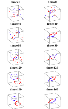
This problem may easily be investigated numerically. The experiments starting from many different random initial distributions give surprising and decidedly counter-intuitive results. Naively, one would expect that this algorithm, when starting from purely random distributions, would just produce more random distributions. However, it turns out that the final configuration depends simply on whether $n$ is even or odd. In case of $n$ even, after roughly $n$ steps of discrete evolution, we get exactly two different separate loops of points. One of these loops contains points with odd labels whereas the other contains points with even labels. On the other hand, in case of $n$ odd we get a single loop of points. All configurations are asymptotically point symmetrical with respect to the origin. (In other words, the center of mass of the system is in the center of coordinates.)

These results may be qualitatively understood. The crucial thing here is that the number of points $n$ is finite and they follow a cyclical pattern. Since the $t$-th order forward derivatives (5) involve $t+1$ terms, when $t$ exceeds $n$ some numbers $x_{i}(0)$ appear more than once. When $t\gg n$ then each $x_{i}(0)$ appears many times in a linear yet complicated combination.

All figures below were made using Mathematica (cf. Fig. 5). We also made some animated gifs which illustrate this phenomenon and are available from the authors.

The statement of the problem was given by the first author. He also performed the numerical experiments described above. The complete analytical solution which we shall present below was given by the second author.

We may consider the coordinates separately. The calculations below concern the $x$ coordinate but may be applied to $y$ (as well as to other possible coordinates in higher dimensions).

Let us denote initial values of coordinates by

$$x_{0}(0),x_{1}(0),\dots,x_{n-1}(0).$$

Recall that the discrete time evolution is described by the equations:

$$\begin{array}[]{l}x_{j}(t+1)=x_{j+1}(t)-x_{j}(t),\qquad t=0,1,\dots,n-2\\ x_{n-1}(t+1)=x_{0}(t)-x_{n-1}(t).\end{array}$$

(6)

The evolution is linear, therefore it may be diagonalized using discrete Fourier transform

$$\hat{x}_{k}(t)=\frac{1}{\sqrt{n}}\sum_{j=0}^{n-1}x_{j}(t)\omega^{-jk},\qquad k=0,1,\dots,n-1,$$

(7)

where $\omega=\exp(2\pi i/n)$. Fourier transform of the eq. (6) reads

$$\hat{x}_{k}(t+1)=(\omega^{k}-1)\hat{x}_{k}(t).$$

(8)

The general formula is

$$\hat{x}_{k}(t)=(\omega^{k}-1)^{t}\hat{x}_{k}(0)$$

(9)

The inverse Fourier transform of eq. (9) is

	$\displaystyle x_{l}(t)$	$\displaystyle=$	$\displaystyle\frac{1}{\sqrt{n}}\sum_{k=0}^{n-1}\hat{x}_{k}(t)\omega^{lk}=\frac{1}{n}\sum_{k=0}^{n-1}(\omega^{k}-1)^{t}\omega^{lk}\sum_{j=0}^{n-1}x_{j}(0)\omega^{-jk}$		(10)
		$\displaystyle=$	$\displaystyle\frac{1}{n}\sum_{k=0}^{n-1}(\omega^{k}-1)^{t}\omega^{lk}\sum_{j=0}^{n-1}x_{j}(0)\omega^{-jk}\qquad l=0,1,\dots,n-1.$

From this point we will write equations for two coordinates.

In the case of odd $n$, absolute value of $|\omega^{k}-1|$ reaches maximum of $r=2\cos(\pi/2n)$ for $k=(n\pm 1)/2$, $\ \omega^{k}=-\exp(\pm\pi i/n)$. Hence for large $t$ we have the following approximation

$$x_{l}(t)\approx r^{t}(-1)^{l+t}\left(\cos\frac{\pi(l+t/2)}{n}\;A+\sin\frac{\pi(l+t/2)}{n}\;B\right)$$

(11)

$$y_{l}(t)\approx r^{t}(-1)^{l+t}\left(\cos\frac{\pi(l+t/2)}{n}\;C+\sin\frac{\pi(l+t/2)}{n}\;D\right)$$

where $A,B,C,D$ are numerical coefficients:

	$\displaystyle A$	$\displaystyle=$	$\displaystyle\frac{2}{n}\sum_{j=0}^{n-1}(-1)^{j}\cos\frac{\pi j}{n}\;x_{j}(0)$		(12)
	$\displaystyle B$	$\displaystyle=$	$\displaystyle\frac{2}{n}\sum_{j=0}^{n-1}(-1)^{j}\sin\frac{\pi j}{n}\;x_{j}(0)$
	$\displaystyle C$	$\displaystyle=$	$\displaystyle\frac{2}{n}\sum_{j=0}^{n-1}(-1)^{j}\cos\frac{\pi j}{n}\;y_{j}(0)$
	$\displaystyle D$	$\displaystyle=$	$\displaystyle\frac{2}{n}\sum_{j=0}^{n-1}(-1)^{j}\sin\frac{\pi j}{n}\;y_{j}(0)$

We note that the following relations hold

	$\displaystyle x_{l}(t+2)$	$\displaystyle=$	$\displaystyle-r^{2}x_{l+1}(t)$		(13)
	$\displaystyle y_{l}(t+2)$	$\displaystyle=$	$\displaystyle-r^{2}y_{l+1}(t).$

We have in this case

$$\left(\begin{array}[]{c}x_{l}\left(t\right)\\ y_{l}\left(t\right)\end{array}\right)\approx r^{t}(-1)^{l+t}\left(\begin{array}[]{cc}A&B\\ C&D\end{array}\right)\left(\begin{array}[]{c}\cos\phi\\ \sin\phi\end{array}\right)$$

(14)

where

$$\phi=\frac{\pi(l+t/2)}{n}$$

Hence for large $t$ and $AD-BC\neq 0$, the points $p_{0}(t),p_{1}(t),\dots,p_{n-1}(t)$ lie on an ellipse

$$(C^{2}+D^{2})x^{2}-2(AC+BD)xy+(A^{2}+B^{2})y^{2}=(AD-BC)^{2}r^{2t}.$$

(15)

In the case of even $n$, absolute value of $|\omega^{k}-1|$ reaches maximum value equal $2$ for $k=n/2$, $\ \omega^{k}=-1$ / Hence for large $t$ we have an approximate relation

	$\displaystyle x_{l}(t)$	$\displaystyle\approx$	$\displaystyle 2^{t}(-1)^{l+t}A$		(16)
	$\displaystyle y_{l}(t)$	$\displaystyle\approx$	$\displaystyle 2^{t}(-1)^{l+t}C,$

where

	$\displaystyle A$	$\displaystyle=$	$\displaystyle\frac{1}{n}\sum_{j=0}^{n-1}(-1)^{j}x_{j}(0)$		(17)
	$\displaystyle C$	$\displaystyle=$	$\displaystyle\frac{1}{n}\sum_{j=0}^{n-1}(-1)^{j}y_{j}(0).$

More detailed investigations, when higher eingenvalue is taken into account, give the following asymptotics:

$$\binom{x_{l}(t)}{y_{l}(t)}\approx(-1)^{l+t}\left[\binom{A}{C}+r_{1}^{t}\left(\begin{array}[]{cc}A_{1}&B_{1}\\ C_{1}&D_{1}\end{array}\right)\binom{\cos\phi}{\sin\phi}\right],\qquad\phi=\frac{2\pi\left(l+\frac{t}{2}\right)}{n}$$

where $r_{1}=2\cos(\pi/n)$ and $A_{1},B_{1},C_{1},D_{1}$ are defined similarly to (12) with $2\pi$ instead of $\pi$.

The process presented in this paper may easily be generalized to more spatial dimensions. The method described in the previous section applies also in this case. Just as in the 2D case the final configuration depends solely on whether $n$ is odd or even (cf. Fig. 4).

Let us finally note that this example of discrete time evolution leading from random to ordered distribution complies with several informal requirements formulated by some distinguished mathematicians when they spoke about aesthetics or even beauty of their discipline. Namely, given result should be easily stated, yet counter-intuitive, deeply non-obvious, surprising. It should have rigorous and elegant proof. Finally – as G. H. Hardy used to emphasize - it should be perfectly useless [3].

Acknowledgement

The authors would like to thank Prof. Marek Wolf, Institute of the Theoretical Physics, University of Wrocław, for stimulating discussion and for performing several independent numerical experiments using Delphi which confirmed the numerical results presented in this paper.

(* Mathematica code *)

(* M random labelled points on the plane *)

M = 25;
ro := Random[Real, {-1,1}, 10]
Table[{ro, ro, ro}, {m, 1, M}];
points = %;

(* differences between consecutive *)
(* vectors generate M new vectors  *)

F[P_] := Table[
  If[k < Length[P], P[[K+1]]-P[[k]],P[[1]]-P[[Length[P]]]],
  {k, 1, Length[P]}
 ]

(* iteration and normalization *)

            Nest[F, points, i]
G[i_] := --------------------------
          Norm[Nest[F, points, i]]

(* color of points: odd - green, even - red *)

b[i_] := If[ OddQ[i], 0.4, 0.0]

(*drawing points *)

H[k_] := Module[
  {t0},
  Show[
   Table[
    Graphics3D[{
      Hue[b[k+i]],
      PointSize[r],
      Point[
       {t0[[i]][[1]], t0[[i]][[2]], t0[[i]][[3]]}]
     }],
    {i, 1, Length[t0]}
   ],
   Background -> RGBColor[0.2, 0.2, 0.3],
   AspectRatio -> 1,
   Axces -> False,
   Boxed -> True,
   PlotRange -> {{-R, +R}, {-R, +R}, {-R, +R}},
   ViewPoint -> {100, -50, 50},
   PlotLabel -> StyleForm["times" <> ToString[k], FontSize -> 12]
 ]

 (* size of dots *)
 r = 0.008;
 (* size of picture *)
 R = 0.13;

 t0 = SessionTime[];
 Table[H[V[k]], {k, 1, 510, 1} ]
 SessionTime[] - t0

 Export["animation.gif", %%, "GIF", ImageResolution -> 100]

References

- [1] Abramowitz, M. and Stegun, I. A. (Eds.), Handbook of Mathematical Functions with Formulas, Graphs, and Mathematical Tables, 9th printing. New York: Dover, p. 877, 1972.
- [2] Arfken, G., Discrete Orthogonality–Discrete Fourier Transform, §14.6 Mathematical Methods for Physicists, 3rd ed. Orlando, FL: Academic Press, pp. 787-792, 1985.
- [3] Hardy, G. H., A Mathematician’s Apology, Cambridge: University Press, 1940.
- [4] R. M. Gray, Toeplitz and Circulant Matrices: A Review, Department of Electrical Engineering, Stanford University
- [5] Weisstein, E., CRC Concise Encyclopedia of Mathematics, second ed., http://mathworld.wolfram.com, Wolfram Research.
- [6] Wolf, M., Example of Order and Disorder: , International Journal of Theoretical Physics, vol. 27, no. 1, 1988.