Stabilizing unstable periodic orbits in the Lorenz equations using time-delayed feedback control

Claire M. Postlethwaite Email: c-postlethwaite@northwestern.edu Affiliation: Engineering Sciences and Applied Mathematics, Northwestern University, Evanston, IL, 60208, USA Mary Silber Affiliation: Engineering Sciences and Applied Mathematics, Northwestern University, Evanston, IL, 60208, USA

August 11, 2026

Abstract

For many years it was believed that an unstable periodic orbit with an odd number of real Floquet multipliers greater than unity cannot be stabilized by the time-delayed feedback control mechanism of Pyragus. A recent paper by Fiedler et al. Fie06 uses the normal form of a subcritical Hopf bifurcation to give a counterexample to this theorem. Using the Lorenz equations as an example, we demonstrate that the stabilization mechanism identified by Fiedler et al. for the Hopf normal form can also apply to unstable periodic orbits created by subcritical Hopf bifurcations in higher-dimensional dynamical systems. Our analysis focuses on a particular codimension-two bifurcation that captures the stabilization mechanism in the Hopf normal form example, and we show that the same codimension-two bifurcation is present in the Lorenz equations with appropriately chosen Pyragus-type time-delayed feedback. This example suggests a possible strategy for choosing the feedback gain matrix in Pyragus control of unstable periodic orbits that arise from a subcritical Hopf bifurcation of a stable equilibrium. In particular, our choice of feedback gain matrix is informed by the Fiedler et al. example, and it works over a broad range of parameters, despite the fact that a center-manifold reduction of the higher-dimensional problem does not lead to their model problem.

Keywords:

control of chaos, delay equations, Lorenz equations, bifurcation theory

pacs

05.45.Gg, 02.30.Ks, 02.30.Oz

I Introduction

Time-delayed feedback control has been used as a method of stabilizing unstable periodic orbits (UPOs) or spatially extended patterns by a number of authors. The method of Pyragus Pyr92, sometimes called ‘time-delayed autosynchronization’ (TDAS), has attracted much attention. Here, the feedback $F$ is proportional to the difference between the current and a past state of the system. That is, $F=K(x(t-\tau)-x(t))$ where $x(t)$ is some state vector, $\tau$ is the period of the targeted UPO and $K$ is a feedback gain matrix. Advantages of this method include the following. First, since the feedback vanishes on any orbit with period $\tau$ , the targeted UPO is still a solution of the system with feedback. Control is therefore achieved in a non-invasive manner. Second, the only information required a priori is the period $\tau$ of the target UPO, rather than a detailed knowledge of the profile of the orbit, or even any knowledge of the form of the original ODEs, which may be useful in experimental setups. The method has been implemented successfully in a variety of laboratory experiments on electronic PT93; GSCS94, laser BDG94, plasma PBA96; FSK02, and chemical SBFHLM93; LFS95 systems, as well as in pattern-forming systems BS96b; MS04; LYH96; PS06; more examples can be found in a recent review by Pyragus Pyr06.

A paper of Nakajima Nak97 gave a supposed restriction on the method of Pyragus. It was believed that if a UPO in a system with no feedback had an odd number of real Floquet multipliers greater than unity, then there was no choice of the feedback gain matrix $K$ for which the method of Pyragus could be used to stabilize the UPO. However, a recent paper of Fiedler et al. Fie06 gives a counterexample to this restriction. They add Pyragus-type feedback to the normal form of a subcritical Hopf bifurcation and show that the subcritical periodic orbit can be stabilized for some values of the feedback gain matrix. The Hopf normal form is two-dimensional, so the subcritical orbit has exactly one unstable Floquet multiplier. The mechanism for stabilizing the orbit is through a transcritical bifurcation with a stable delay-induced periodic orbit. Just et al. Jus07 investigate a series of bifurcations in this system, which has the attractive feature that, despite the presence of the delay terms, much of the analysis can be carried out analytically.

The subcritical Hopf bifurcation of a stable equilibrium is a generic mechanism for creating UPOs with an odd number of unstable Floquet multipliers. Such bifurcations occur in a number of physical systems, such as the Belousov–Zhabotinsky reaction-diffusion equation IHS97, the Hodgkin–Huxley model of action potentials in neurons GW00, and in NMR lasers BHL89. The reduction of these higher-dimensional dynamical systems to the two-dimensional normal form of the Hopf bifurcation problem is a standard procedure MM76; GH83. Moreover, if Pyragus-type feedback delay terms were added to the model ODEs, then these (infinite-dimensional) dynamical systems could likewise be reduced to the standard two-dimensional normal form in a vicinity of a Hopf bifurcation HL93, with the parameters of the feedback control matrix $K$ modifying the coefficients in the normal form. Despite this disconnect between center manifold reduction of delay equations to Hopf normal form, and the example of Fiedler et al. in which the feedback delay terms are added directly to the Hopf normal form, we find that the same stabilization mechanism of subcritical Hopf orbits applies to both their example and to the one we present for the Lorenz equations.

Specifically, we study a subcritical Hopf bifurcation of a stable equilibrium in the Lorenz equations L63; Spa82, and show that Pyragus-type feedback can stabilize the subcritical periodic orbit. As in the example in Fie06, in the absence of feedback, the bifurcating periodic orbit has exactly one real unstable Floquet multiplier. It also has one stable Floquet multiplier, and one Floquet multiplier equal to one (corresponding to the neutral direction along the orbit). The $3\times 3$ gain matrix multiplying the Pyragus feedback terms can be chosen in many different ways. We give two examples in which we choose the structure of the gain matrix in different ways and show that they give quite different results.

In our first example, we choose the gain matrix in a manner suggested by the results in Fie06 and Jus07: there is no feedback in the stable direction of the UPO, and Pyragus-type feedback in the direction of the unstable Floquet multiplier, which is identical in form to the feedback in Fie06. In this way, the problem of choosing the nine parameters in the $3\times 3$ gain matrix is reduced to one of making an informed choice of the two parameters employed in Fie06. We find that the subcritical orbit can be stabilized over a wide range of values of our two bifurcation parameters: the amplitude of the feedback gain, and the usual control parameter $\rho$ in the Lorenz equations. We identify a codimension-two point in the Hopf normal form example, where two Hopf bifurcations collide, and show that the same codimension-two point can be found in the Lorenz system with this choice of feedback, and the bifurcation structure is qualitatively the same in the two cases. This codimension-two point captures the stabilization mechanism in both examples: the periodic orbits created by the two Hopf bifurcations exchange stability in a transcritical bifurcation. The curve of transcritical bifurcations in our two-parameter plane emanates from the Hopf-Hopf codimension-two point.

Our second choice of the gain matrix is a real multiple of the identity. This is also a natural choice, but in contrast with our first example we show that here the subcritical orbit cannot be stabilized for any parameters close to the original Hopf bifurcation. Our two bifurcation parameters are again the amplitude of the gain and the parameter $\rho$ in the Lorenz equations. We give analytical results on the location of Hopf bifurcation curves and hence deduce the stability of the periodic orbit as it bifurcates.

This paper is organized as follows. In section II we review some results from Fiedler et al. Fie06 and Just et al. Jus07. In section III we give our example system of the Lorenz equations with Pyragus feedback. We give two examples of the choice of gain matrix. We explain for the first example how we choose the gain matrix to stabilize the subcritical Hopf orbit, and show that the bifurcation structure of this system is the same as that for the normal form system. For the second example, the gain matrix is a real multiple of the identity and we show that the subcritical orbit cannot be stabilized. Section IV concludes.

II The Hopf normal form with delay

In this section we recap the results of Fie06 and identify a particular codimension-two point in the Hopf normal form with delay which we will later examine for the Lorenz equations with feedback. This codimension-two point acts as an organizing center for the bifurcations involved in the mechanism for stabilizing the periodic orbit.

The normal form of a subcritical Hopf bifurcation with a Pyragus-type delay term is:

\dot{z}(t)=(\lambda+i)z(t)+(1+i\gamma)|z(t)|^{2}z(t)+b(z(t-\tau)-z(t))

(1)

with $z\in\mathbb{C}$ , and parameters $\lambda,\gamma\in\mathbb{R}$ . The feedback gain $b=b_{0}\mathrm{e}^{i\beta}\in\mathbb{C}$ , and the delay $\tau>0$ . The linear Hopf frequency has been normalized to unity by an appropriate scaling of time. We consider $\lambda$ as the primary bifurcation parameter. We consider only $\gamma<0$ ; this is the case in the Lorenz example.

For the system with no feedback (i.e. $b=0$ ) we can write $z=r\mathrm{e}^{i\theta}$ and then

	$\displaystyle\dot{r}$	$\displaystyle=(\lambda+r^{2})r,$		(2)
	$\displaystyle\dot{\theta}$	$\displaystyle=1+\gamma r^{2}.$		(3)

Periodic orbits exist with amplitude $r^{2}=-\lambda$ if $\lambda<0$ , so $\dot{\theta}=1-\gamma\lambda$ and the orbits have minimal period $T=2\pi/(1-\gamma\lambda)$ . We refer to these orbits as the Pyragus orbits, and it is these orbits that we wish to stabilize non-invasively by adding an appropriate feedback term (i.e. with $b\neq 0$ ).

Following Fie06 and Jus07, we define the Pyragus curve $\tau=\tau_{P}(\lambda)$ in $\lambda$ - $\tau$ space, along which the feedback vanishes on the Pyragus orbits:

\tau_{P}(\lambda)=\frac{2\pi}{1-\gamma\lambda}.

(4)

We plot this curve in $\lambda$ - $\tau$ space in figure 1, along with curves of Hopf bifurcations from the zero solution. In later sections, we set $\tau=\tau_{P}(\lambda)$ , as our main purpose is the non-invasive stabilization of the Pyragus orbits.

The zero solution of (1) undergoes Hopf bifurcations when the characteristic equation has purely imaginary solutions. Setting $z(t)=\mathrm{e}^{\eta t}$ in (1) and linearizing we find:

\eta=\lambda+i+b(\mathrm{e}^{\eta\tau}-1).

Writing $\eta=i\omega$ and separating into real and imaginary parts gives

	$\displaystyle 0$	$\displaystyle=\lambda+b_{0}[\cos(\beta-\omega\tau)-\cos\beta],$		(5)
	$\displaystyle\omega-1$	$\displaystyle=b_{0}[\sin(\beta-\omega\tau)-\sin\beta].$		(6)

These equations define the Hopf curves $\tau=\tau_{H}(\lambda)$ , in $\lambda$ - $\tau$ space, parameterized by the linear frequency $\omega$ associated with the bifurcating periodic orbit. There are multiple branches to this curve, which we show in figure 1(a), but we concentrate on the one which intersects the curve $\tau=\tau_{P}(\lambda)$ at $(\lambda,\tau)=(0,2\pi)$ . The solution of the characteristic equation at $\lambda=0$ , $\tau=2\pi$ has $\omega=1$ and corresponds to the Hopf bifurcation to the Pyragus orbit.

Figure 1 shows the possible configurations of the curves $\tau=\tau_{P}(\lambda)$ and $\tau=\tau_{H}(\lambda)$ as the parameter $b_{0}$ is varied.

The curves typically cross in two places: at $\lambda=0$ , and at a second location depending on $b_{0}$ . At $b_{0}=b_{0}^{c}$ , the two curves are tangent at $\lambda=0$ and only intersect once. Just et al. Jus07 show that

b_{0}^{c}=\frac{-1}{2\pi(\gamma\sin\beta+\cos\beta)}.

For simplicity, we assume $b_{0}^{c}>0$ , so we must have $\gamma\sin\beta+\cos\beta<0$ .

We define a curve of Hopf bifurcations $b_{0}=b_{0}^{\mathrm{Hopf}}(\lambda)$ in $\lambda$ - $b_{0}$ space by the location of the second intersection of $\tau_{P}(\lambda)$ and $\tau_{H}(\lambda)$ . This is a Hopf bifurcation to a delay-induced periodic orbit, that is, a periodic orbit arising from the addition of the delay terms; one for which the feedback does not vanish.

We adopt the convention that a Hopf bifurcation of a stable equilibrium is called ‘supercritical’ (‘subcritical’) if the resulting periodic orbit bifurcates into the parameter regime where it coexists with the unstable (stable) equilibrium. Such a supercritical bifurcation generically produces a stable periodic orbit GH83, while the subcritical case produces an unstable periodic orbit. In the absence of feedback, the bifurcating orbit is subcritical and unstable. The mechanism for stabilization involves the additional delay-induced Hopf bifurcation at $b_{0}^{\mathrm{Hopf}}(\lambda)$ . This bifurcation can change the trivial equilibrium from being stable to being unstable. Consequently, the Pyragus orbit may then co-exist with an unstable periodic orbit. As the Hopf bifurcation at $b_{0}^{\mathrm{Hopf}}(\lambda)$ passes through $\lambda=0$ , the original Hopf bifurcation to the Pyragus orbit at $\lambda=0$ changes from a subcritical one to a supercritical one. This is all done without otherwise altering the form of the Pyragus orbit.

The Hopf bifurcation of the zero solution to the Pyragus orbit at $(\lambda,\tau)=(0,2\pi)$ changes from subcritical to supercritical as described above as $b_{0}$ is increased through $b_{0}^{c}$ , since for $b_{0}>b_{0}^{c}$ , the curve $\tau_{P}(\lambda)$ lies ‘inside’ $\tau_{H}(\lambda)$ . In this sense, $b_{0}^{c}$ is the smallest value of the feedback gain for which the Pyragus orbit is stabilized immediately after the bifurcation point. The minimum positive $b_{0}^{c}$ can be selected by choosing $\beta$ such that $\gamma=\tan\beta$ .

II.1 A codimension-two bifurcation point

We now review some of the details of the bifurcation structure of the system (1) which are described in Just et al. Jus07, and identify the codimension-two point we examine in the Lorenz system. We consider $\lambda$ and $b_{0}$ as two bifurcation parameters, and fix $\tau=\tau_{P}(\lambda)$ .

The mechanism by which the Pyragus orbit is stabilized is through a transcritical bifurcation with a delay-induced periodic orbit. As shown in Just et al. Jus07, the transcritical bifurcations occur when

\tau=\frac{-1}{b_{0}(\cos\beta+\gamma\sin\beta)},

or, in $\lambda$ - $b_{0}$ space, since $\tau=\tau_{P}(\lambda)$ , when

\lambda=\frac{1}{\gamma}(1+2\pi b_{0}(\cos\beta+\gamma\sin\beta))=\frac{1}{\gamma}\left(1-\frac{b_{0}}{b_{0}^{c}}\right).

This line of transcritical bifurcations collides in $\lambda$ - $b_{0}$ space with the two curves of Hopf bifurcations $\lambda=0$ and $b_{0}=b_{0}^{\mathrm{Hopf}}(\lambda)$ at $(\lambda,b_{0})=(0,b_{0}^{c})$ , at a double-Hopf codimension-two point.

In figure 2 we sketch the bifurcation structure around this point in $\lambda$ - $b_{0}$ space. From this figure we can see that in order for the Pyragus orbit to bifurcate stably (i.e. supercritically) at $\lambda=0$ , we must have $b_{0}>b_{0}^{c}$ .

III The Lorenz Equations with time-delayed feedback

We now use the Lorenz equations as an example system to demonstrate that the feedback described above can also stabilize orbits arising in a subcritical Hopf bifurcation in a higher-dimensional system of differential equations. We give two examples of a choice of feedback gain matrix. The first choice is informed by the results given above, and for the second choice we set the gain matrix equal to a real multiple of the identity. In the first example, we further locate the codimension-two point described in section II.1, in the Lorenz system with feedback, and show that the bifurcation structure is the same as in the normal form case.

The Lorenz equations L63; Spa82 are most often written in the following form:

	$\displaystyle\dot{x}$	$\displaystyle=\sigma(y-x),$
	$\displaystyle\dot{y}$	$\displaystyle=\rho x-y-xz,$
	$\displaystyle\dot{z}$	$\displaystyle=-\alpha z+xy,$

for real parameters $\sigma$ , $\alpha$ and $\rho$ . Lorenz and most other authors studied the parameter regime $\sigma=10$ , $\alpha=8/3$ , $\rho>0$ , and we continue in the same manner. Taking $\rho$ as the primary bifurcation parameter, the zero solution is stable for $\rho<1$ and loses stability in a supercritical pitchfork bifurcation at $\rho=1$ . Two further equilibria are created at

\vec{x}_{\pm}=(\pm\sqrt{(\alpha(\rho-1))},\pm\sqrt{(\alpha(\rho-1))},\rho-1).

As $\rho$ is increased further, these equilibria each undergo a subcritical Hopf bifurcation at $\rho_{h}=\sigma(\sigma+\alpha+3)/(\sigma-\alpha-1)\approx 24.74$ (see GH83 and MM76 for further details). It is this bifurcation that we study in the following, so we shift coordinates to be centered around $\vec{x}_{+}$ and rescale to obtain:

$\displaystyle\dot{u}$	$\displaystyle=\sigma(v-u),$
$\displaystyle\dot{v}$	$\displaystyle=u-v-(\rho-1)w-(\rho-1)uw,$	(7)
$\displaystyle\dot{w}$	$\displaystyle=\alpha(u+v-w+uv).$

Figure 3 shows a bifurcation diagram of the subcritical bifurcation of the zero solution of (7), and also the period $T$ of the bifurcating orbits, which we use to determine the delay time $\tau_{P}(\rho)$ in the controlled system. The periodic orbit exists for $13.926<\rho<\rho_{h}$ ; at the lower boundary it collides with a fixed point in a homoclinic bifurcation.

III.1 Adding time-delayed feedback

We now add Pyragus-type feedback to the Lorenz equations. We write

\begin{pmatrix}\dot{u}\\ \dot{v}\\ \dot{w}\end{pmatrix}=J(\rho)\begin{pmatrix}u\\ v\\ w\end{pmatrix}+N(u,v,w)+\Gamma\begin{pmatrix}u_{\tau}-u\\ v_{\tau}-v\\ w_{\tau}-w\end{pmatrix},

(8)

where

J(\rho)=\begin{pmatrix}-\sigma&\sigma&0\\ 1&-1&-(\rho-1)\\ \alpha&\alpha&-\alpha\end{pmatrix},\qquad N(u,v,w)=\begin{pmatrix}0\\ -(\rho-1)uw\\ \alpha uv\end{pmatrix},

(9)

$u_{\tau}=u(t-\tau)$ , etc. and $\Gamma$ is a $3\times 3$ real feedback gain matrix, to be determined. In this section we use the results of Fie06 and Jus07 to inform our choice of the control matrix $\Gamma$ . In general, $\Gamma$ would contain nine independent parameters, but the method we describe reduces this to only two. In section III.3 we describe the dynamics when $\Gamma$ is a real multiple of the identity. Note that if this system were reduced to normal form around the Hopf bifurcation point, the resulting equations would not be the same as (1). That is, there would be no delay terms; the delay terms here would only have the affect of altering the parameters in the usual Hopf normal form. See HL93 for more details.

At the bifurcation point ( $\rho=\rho_{h}$ ), $J$ has one real negative eigenvalue (which we denote by $-\lambda_{h}=-\alpha-\sigma-1\approx-11.7$ ), and a pair of purely imaginary eigenvalues ( $\pm i\omega_{h}$ , $\omega_{h}=\sqrt{(2\alpha\sigma(\sigma+1))/(\sigma-\alpha-1)}\approx 9.62$ ). The center manifold of the original problem with no feedback is therefore two-dimensional, and the eigenvectors of $J$ can be found explicitly (see MM76). Close to the bifurcation point, the subcritical orbit will lie in a two-dimensional manifold which is close to the center subspace at the bifurcation point. We therefore choose

\Gamma=EGE^{-1},

where $E$ is the matrix of eigenvectors which puts $J(\rho_{h})=J_{h}$ in Jordan normal form, that is

E^{-1}J_{h}E=\begin{pmatrix}-\lambda_{h}&0&0\\ 0&0&-\omega_{h}\\ 0&\omega_{h}&0\end{pmatrix},

(10)

and

G=\begin{pmatrix}0&0&0\\ 0&b_{0}\cos\beta&-b_{0}\sin\beta\\ 0&b_{0}\sin\beta&b_{0}\cos\beta\end{pmatrix}.

(11)

There is then no feedback in the stable direction, and Pyragus-type feedback in the directions tangent to the center manifold.

In the following numerical results, we set $\beta=\pi/4$ , as in Fiedler et al., and vary $b_{0}$ .

III.2 Numerical results

We use the continuation package DDE-BIFTOOL ddebiftool to analyze the delay-differential equation (8). The primary bifurcation parameter is $\rho$ , with the subcritical Hopf bifurcation for the system without feedback occurring at $\rho=\rho_{h}\approx 24.74$ . Recall we have set $\sigma=10$ , $\alpha=8/3$ and $\beta=\pi/4$ .

First, we locate Hopf bifurcations of the trivial solution in the $\rho$ - $\tau$ plane, for various values of $b_{0}$ .

Figure 4 shows curves of Hopf bifurcations $\tau=\tau_{H}(\rho)$ for $b_{0}=1.2$ and $b_{0}=0.1$ . We also plot the curve $\tau=\tau_{P}(\rho)$ , given by the period of the bifurcating subcritical orbits (see figure 3). Figure 4 is qualitatively similar to figure 1 (the corresponding figure for the normal form case). For $b_{0}=1.2$ , $\tau_{P}(\rho)$ lies inside $\tau_{H}(\rho)$ , and so we expect, by analogy with the normal form case, that choosing $\tau=\tau_{P}(\rho)$ will stabilize the Pyragus orbit. For $b_{0}=0.1$ , $\tau_{P}(\rho)$ lies outside $\tau_{H}(\rho)$ , and so the feedback cannot stabilize the Pyragus orbit near onset, since it bifurcates subcritically (i.e. it coexists with the stable equilibrium from which it bifurcates). The codimension-two point occurs at some value of $b_{0}$ that is the boundary between these cases.

We use DDE-BIFTOOL to locate this codimension-two point. As in the normal form case, we set $\tau=\tau_{P}(\rho)$ . We do not have an analytic form for $\tau_{P}(\rho)$ , so we numerically estimate $\tau_{P}(\rho)$ in the following way. For $\rho<\rho_{h}$ we set $\tau_{P}(\rho)$ equal to the period of the bifurcating period orbits for the system with no feedback (see figure 3). We want to continue $\tau_{P}(\rho)$ into $\rho>\rho_{h}$ , so we can complete both sides of the bifurcation diagram, so here we set $\tau_{P}(\rho)=\tau_{h}/(1-B(\rho-\rho_{h}))$ , where $B=-0.0528$ , and $\tau_{h}=\tau_{P}(\rho_{h})\approx 0.6528$ . This choice of $B$ ensures that $\tau_{P}(\rho)$ is continuous and has continuous first derivative at $\rho=\rho_{h}$ .

With the parameter restriction $\tau=\tau_{P}(\rho)$ , we generate curves of Hopf bifurcations from the zero solution in the $\rho$ - $b_{0}$ plane; these are shown in figure 5.

We can then estimate the location of the codimension-two point, at $(\rho,b_{0})=(\rho_{h},b_{0}^{c})$ , the point where the two curves of Hopf bifurcations cross. We find $b_{0}^{c}\approx 0.221$ . We follow a path around the codimension-two point and track the amplitude and stability of the bifurcating periodic orbits; a bifurcation diagram of the periodic orbits is shown in figure 5. The transcritical bifurcation of periodic orbits can clearly be seen. Note that figure 5 is qualitatively similar to figure 2, showing that the bifurcation structure in the normal form case, and in our Lorenz example are the same.

With the additional feedback, the Pyragus orbits are stable for a wide parameter range.

In figure 6, we show the stability of the Pyragus orbits as $\rho$ and $b_{0}$ are varied. The transcritical bifurcation can be seen as the boundary of the stable region which terminates at the codimension-two point. The orbits also undergo an instability at around $\rho\approx 17$ . Along this boundary of the stable region, the periodic orbits have a Floquet multiplier equal to $-1$ , and so the instability is a period-doubling bifurcation.

In figure 7 we show results of forward time integration of the delay-differential equation (8), at $\rho=23<\rho_{h}$ , with $\tau=\tau_{P}(\rho)=0.7191$ . Initally, $b_{0}=1.2$ , and the Pyragus orbit is stable. The feedback is then turned off (i.e. $b_{0}=0$ ) at $t=50$ , and the trajectory decays back to the zero solution. We have used DDE-BIFTOOL to confirm the stability of these orbits.

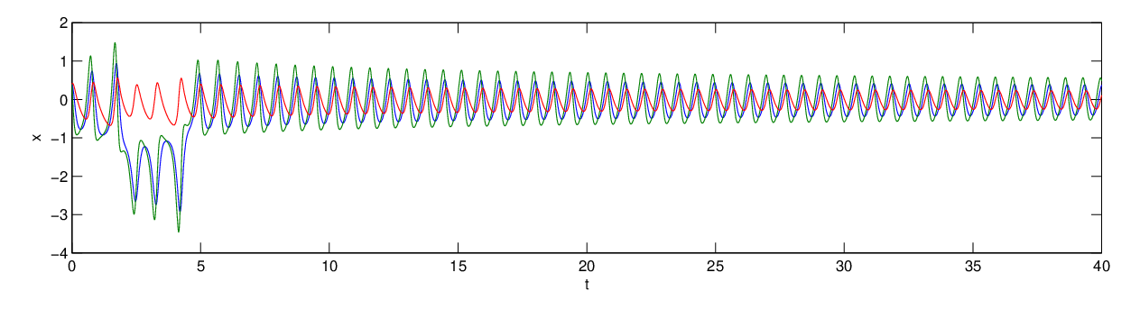
The structure around the codimension-two point also tells us that the delay-induced orbits can be stable in the region $\rho>\rho_{h}$ . For example, at $\rho=24.8388$ , $b_{0}=0.22$ , $\tau=0.6494$ , we can use DDE-BIFTOOL to show that there exists a stable delay-induced periodic orbit with a period of $0.6537$ . Figure 8 shows time integration at these parameter values, with feedback turned on at $t=5$ . The figure shows the chaotic attractor for $t<5$ and an approach to a stable periodic orbit for $t>5$ .

III.3 A second example

Another natural choice for the gain matrix $\Gamma$ is a real multiple of the identity. As a comparison to the results given above, we now consider this case, so write

\Gamma=b_{0}\begin{pmatrix}1&0&0\\ 0&1&0\\ 0&0&1\end{pmatrix},\qquad b_{0}\in\mathbb{R}.

(12)

For this choice of $\Gamma$ we can obtain analytical results, and we show that the bifurcation structure is different from our previous example, whatever the value of $b_{0}$ . We show first that unstable periodic orbits with real positive Floquet exponents cannot be stabilised using this form of feedback. We then discuss the shape and location of the curves of Hopf bifurcation from the origin, in a similar manner to the previous section, to give a comparison of the two types of feedback. The codimension-two point described previously does not exist, and the Hopf bifurcation to the Pyragus orbit is always subcritical. That is, the periodic orbit in $\rho<\rho_{h}$ always bifurcates unstably from an equilibrium which is stable in $\rho<\rho_{h}$ and unstable in $\rho>\rho_{h}$ .

Consider a Pyragus solution $\vec{u}^{\star}(t)$ of (8), which is periodic with period $\tau$ , and with $\Gamma$ as in (12). Then if $\mu$ is a Floquet exponent of $\vec{u}^{\star}$ (in the system with no feedback), the characteristic equation for $\vec{u}^{\star}$ in the system with feedback is given by

(\lambda-b_{0}(\mathrm{e}^{-\lambda\tau}-1))=\mu.

(13)

Both here, and in the analysis which follows below, simplification is possible because $\Gamma$ is a multiple of the identity. If $\vec{u}^{\star}$ has one Floquet exponent $\mu$ which is real and positive, then it can be shown (see e.g. BC63) that there always exists at least one solution $\lambda$ which is real and positive. Hence stabilization of $\vec{u}^{\star}$ cannot be achieved.

We note that at the subcritical Hopf bifurcation from the zero solution in (7), the orbit which bifurcates has one real stable multiplier (inherited from the zero solution) and one neutral multiplier, and so the remaining unstable multiplier must be real. Therefore the Pyragus orbit cannot be stabilized close to the Hopf bifurcation using this type of feedback.

In addition, we now follow the method of the previous section to find curves of Hopf bifurcations of the zero solution of (8) in $\rho$ - $\tau$ space. This provides us with a comparison of the two types of feedback used in this and the previous section. We are particularly interested in those curves which pass through $(\rho,\tau)=(\rho_{h},\tau_{h})$ , with Hopf frequency equal to $\omega_{h}$ , as this is the Hopf bifurcation to the Pyragus orbit.

Consider the linearisation of (8) about the origin, and write $(u,v,w)^{T}=\vec{u}\mathrm{e}^{\lambda t}$ . Then

\lambda\vec{u}\mathrm{e}^{\lambda t}=J(\rho)\vec{u}\mathrm{e}^{\lambda t}+\Gamma\vec{u}(\mathrm{e}^{-\lambda\tau}-1)\mathrm{e}^{\lambda t},

and so for a non-trivial solution ( $\vec{u}\neq\vec{0}$ ) to exist, $\lambda$ must satisfy the characteristic equation:

\det[(\lambda-b_{0}(\mathrm{e}^{-\lambda\tau}-1))I-J(\rho)]=0.

(14)

Note that we have been able to simplify this equation because in this example $\Gamma$ is a multiple of the identity. This tells us that $g(\lambda)\equiv(\lambda-b_{0}(\mathrm{e}^{-\lambda\tau}-1))$ are the eigenvalues of $J(\rho)$ .

When $\rho$ is close to $\rho_{h}$ , $J(\rho)$ has one negative eigenvalue $-\lambda_{1}(\rho)$ , and a complex conjugate pair we denote as $\mu(\rho)\pm i\nu(\rho)$ . Note that $\mu(\rho_{h})=0$ , and $\nu(\rho_{h})=\omega_{h}$ .

We find curves of Hopf bifurcations in $\rho$ - $\tau$ space, by writing $\lambda=i\omega$ ( $\omega\in\mathbb{R}$ ) and setting $g(i\omega)$ equal to the eigenvalues of $J(\rho)$ , $\mu(\rho)+i\nu(\rho)$ . We note that setting $g(i\omega)$ equal to the negative eigenvalue of $J(\rho)$ , $-\lambda_{1}(\rho)$ , does not produce any Hopf curves which pass through $(\rho,\tau)=(\rho_{h},\tau_{h})$ , so we do not consider these here. Equating real and imaginary parts gives

	$\displaystyle-b_{0}(\cos(\omega\tau)-1)$	$\displaystyle=\mu(\rho),$		(15)
	$\displaystyle\omega+b_{0}\sin(\omega\tau)$	$\displaystyle=\nu(\rho).$		(16)

Equations (15) and (16) describe curves of Hopf bifurcations in $\rho$ - $\tau$ space, parameterized by the Hopf frequency $\omega$ .

Figure 9 shows examples of the shape of these Hopf curves; compare with figure 4 showing the Hopf curves in our previous example. The zero solution is unstable to the right of the curves and stable to the left of the curves. We now explain why we expect the curves to have this shape.

We have:

(\nu(\rho)-\omega)^{2}=\mu(\rho)(2b_{0}-\mu(\rho)).

Note that we need $\mu(\rho)(2b_{0}-\mu(\rho))\geq 0$ for solutions to exist. That is, if $b_{0}>0$ , we need $0\leq\mu(\rho)\leq 2b_{0}$ , and if $b_{0}<0$ , we need $2b_{0}\leq\mu(\rho)\leq 0$ . Since $\mu(\rho)$ is a monotonically increasing function over the range of $\rho$ we are considering, this gives a connected range of $\rho$ for which Hopf bifurcations can occur, with boundaries at $\rho=\rho_{h}$ (since $\mu(\rho_{h})=0$ ) and at $\rho=\rho^{\star}(b_{0})$ (where $\mu(\rho^{\star})=2b_{0}$ ). Note that at $\rho=\rho_{h}$ , $\omega=\nu(\rho_{h})=\omega_{h}$ , and so this is the Hopf bifurcation to the Pyragus orbit.

The solutions for $\tau$ along the Hopf curve solve

\cos(\omega\tau)=1-\frac{\mu(\rho)}{b_{0}}.

Since $\mu(\rho_{h})=0$ , at $\rho=\rho_{h}$ , $\omega\tau=2\pi n$ , and similarly since $\mu(\rho^{\star})=2b_{0}$ , at $\rho=\rho^{\star}$ , $\omega\tau=\pi(2n+1)$ . The curve of Hopf bifurcations is thus tangent to the lines $\rho=\rho_{h}$ and $\rho=\rho^{\star}$ , and forms a series of wiggles between these value of $\rho$ . In particular, the curve is tangent to $\rho=\rho_{h}$ at $(\rho,\tau)=(\rho_{h},\tau_{h}$ ), where $\omega=\omega_{h}$ , the Hopf bifurcation to the Pyragus orbit.

Therefore, for any value of $b_{0}$ , the Pyragus curve $\tau=\tau_{P}(\rho)$ (which originates at $(\rho,\tau)=(\rho_{h},\tau_{h})$ , and is also shown in figure 9), will always be to the left of the Hopf curves at $\rho=\rho_{h}$ . The zero equilibrium is therefore stable along the Pyragus curve close to the bifurcation point in $\rho<\rho_{h}$ , and so the Pyragus orbit will always bifurcate unstably. Figure 10 shows a contour plot of the largest Floquet multipliers of the periodic orbit, as $\rho$ and $b_{0}$ are varied. For all values shown the periodic orbit is unstable.

IV Discussion

In this paper, we have demonstrated how the mechanism used by Fiedler et al. Fie06 for stabilizing periodic orbits with one unstable Floquet multiplier carries over to higher dimensional systems, using the Lorenz equations as an example. We use the results from their idealized example to inform our choice of the feedback gain matrix, and this method follows a set prescription which we expect could be used on other systems. First we find the two-dimensional linear center eigenspace of the system with no feedback at the Hopf bifurcation point. Feedback is then added in the directions lying tangent to this center subspace, using a $2\times 2$ gain matrix of the form given by Fiedler et al. This then leaves only the two parameters $\beta$ and $b_{0}$ to be chosen. For the example of the Lorenz equation, the subcritical orbits are stabilized over a wide range of parameters. We contrast this with an example of choosing the gain matrix as a real multiple of the identity. In this case the Pyragus orbit could not be stabilised.

Choosing the gain matrix for our Lorenz equations example required a knowledge of the linearization of the system at the bifurcation point. This method may also be applicable in systems for which the governing equations are not known, if it is possible to access perturbations to the equilibrium solution near the Hopf bifurcation point, and hence extract the unstable eigenvectors numerically from experimental data.

We have additionally shown that the Lorenz equations example contains a codimension-two point which is also present in the normal form example of Fie06. This double-Hopf point is not generic. In the normal form example of Fie06 there is an additional $SO(2)$ symmetry which is not present in the Lorenz example. Additional structures in the problem force a normally codimension-three phenomena GKL90 to be codimension-two, since the frequencies of the bifurcating periodic orbits are forced to be in one:one resonance at the codimension-two point. It would be of interest to examine this degeneracy in more detail, by understanding the mathematics behind the structure of the Hopf-Hopf bifurcation in these examples. We intend to investigate further examples to see how robust this bifurcation structure is, for example, whether it appears in say, the Hodgkin–Huxley GW00 or Belousov–Zhabotinsky IHS97 examples.

Acknowledgements

The authors would like to thank Luis Mier-y-Teran and David Barton for assistance with DDE-BIFTOOL. We are grateful to an anonymous referee for several helpful and detailed suggestions. This research was funded by NSF grant DMS-0309667.

References

(1) K. Pyragas, Phys. Letts. A,170, 421–428, (1992).
(2) K. Pyragas and A. Tamaševičius, Phys. Letts. A, 180, 99, (1993).
(3) D. J. Gauthier, D. W. Sukow, H. M. Concannon and J. E. S. Socolar, Phys. Rev. E, 50, 2343 (1994).
(4) S. Bielawski, D. Derozier and P. Glorieux, Phys. Rev. E, 49, R971 (1994).
(5) Th. Pierre, G. Bonhomme and A. Atipo Phys. Rev. Lett., 76, 2290 (1996).
(6) T. Fukuyama, H. Shirahama and Y. Kawai, Physics of Plasmas, 9, 4525 (2002).
(7) F. W. Schneider, R. Blittersdorf, A. Förster, T. Hauck, D. Lebender and J.Müller, J. Phys. Chem., 97, 12244 (1993).
(8) A. Lekebusch, A. Förster and F.W. Schneider, J. Phys. Chem., 99, 681 (1995).
(9) M.E. Bleich, J.E.S. Socolar, Phys. Rev. E, 54(1) R17–R20 (1996).
(10) K. Montgomery and M. Silber, Nonlinearity, 17(6), 2225-2248 (2004).
(11) W. Lu, D. Yu, R. G. Harrison, Phys. Rev. Letts., 76(18), 3316–3319 (1996).
(12) C. M. Postlethwaite and M. Silber, Physica D (2007) in press. arXiv:nlin/0701007v1
(13) K. Pyragas, Phil. Trans. R. Soc. A, 364, 2309–2334 (2006).
(14) H. Nakajima, Phys. Letts. A, 232, 207–210 (1997).
(15) B. Fiedler, V. Flunkert, M. Georgi, P. Hovel and E.Scholl, Phys. Rev. Lett., 98, 114101 (2007).
(16) W. Just, B. Fiedler, M. Georgi, V. Flunkert, P. Hovel and E.Scholl, Phys. Rev. E (2007) in press.
(17) M. Ipsen, F. Hynne, P. G. Sorensen, Int. J. Bif. Chaos, 7, 1539–1554 (1997).
(18) J. Guckenheimer and A. R. Willms, Physica D, 139, 195–216 (2000).
(19) A. Baugher, P. Hammack, J. Lin, Phys. Rev. A. 39 (3) 1549–1551 (1989).
(20) J. Guckenheimer and P. Holmes, Nonlinear Oscillations, dynamical systems, and bifurcations of vector fields. Appl. Math. Sci. Ser. 42, (Springer-Verlag, New York, 1983).
(21) J.E. Marsden and M. McCracken, The Hopf bifurcation and its applications. Appl. Math. Sci. Ser. 19, (Springer-Verlag, New York, 1976).
(22) J. Hale and S. Verduyn Lunel, Introduction to Functional Differential Equations, (Springer–Verlag, New York, 1993).
(23) E. N. Lorenz, J. Atmos. Sci., 20, 130–141 (1963).
(24) C. Sparrow, The Lorenz Equations: bifurcations, chaos and strange attractors, (Springer, 1982).
(25) K. Engelborghs, T. Luzyanina and G. Samaey, DDE-BIFTOOL v. 2.00 user manual: a Matlab package for bifurcation analysis of delay differential equations, Technical Report TW-330, Department of Computer Science, K.U.Leuven, Leuven, Belgium, (2001).
(26) R. Bellman and K. L. Cooke, Differential-Difference Equations, (Academic Press, 1963).
(27) S. A. van Gils, M. Krupa and W. F Langford, Nonlinearity 3, 825–850 (1990).