We construct the metric of new multi-black hole configurations on a $d$ -dimensional cylinder $\mathbb{R}^{d-1}\times S^{1}$ , in the limit of small total mass (or equivalently in the limit of a large cylinder). These solutions are valid to first order in the total mass and describe configurations with several small black holes located at different points along the circle direction of the cylinder. We explain that a static configuration of black holes is required to be in equilibrium such that the external force on each black hole is zero, and we examine the resulting conditions. The first-order corrected thermodynamics of the solutions is obtained and a Newtonian interpretation of it is given. We then study the consequences of the multi-black hole configurations for the phase structure of static Kaluza-Klein black holes and show that our new solutions imply continuous non-uniqueness in the phase diagram. The new multi-black hole configurations raise the question of existence of new non-uniform black strings. Finally, a further analysis of the three-black hole configuration suggests the possibility of a new class of static lumpy black holes in Kaluza-Klein space.

1 Introduction

Black holes in four-dimensional General Relativity have a very simple phase structure. The uniqueness theorems for pure gravity assert that the only possible stationary black hole solution for a given mass and angular momentum is the Kerr black hole.

For higher-dimensional General Relativity, the situation is vastly different. In particular, if we imagine that we live in a world which is five dimensional with the extra dimension curled up on a circle, the relevant black hole solutions are those which asymptote to four-dimensional Minkowski-space times a circle ( $\mathcal{M}^{4}\times S^{1}$ ), $i.e.$ the five-dimensional Kaluza-Klein space-times. The phase structure of such black holes has been shown to be very rich and contains phases with event horizons of different topology and even phases where Kaluza-Klein bubbles are attached to black holes [1, 2, 3]. More generally, we get a similarly rich phase structure for the case of black holes asymptoting to $d$ -dimensional Minkowski-space times a circle ( $\mathcal{M}^{d}\times S^{1}$ ) with $d\geq 4$ .¹¹ 1 Note that the case $\mathcal{M}^{3}\times S^{1}$ studied in [4, 5, 6, 7] is different due to the high amount of symmetry. The spatial part of this space-time is a $d$ -dimensional cylinder $\mathbb{R}^{d-1}\times S^{1}$ .

The two static black hole phases which most obviously should appear for $\mathcal{M}^{d}\times S^{1}$ are the localized black hole phase, which for small mass behaves as a $d+1$ dimensional Schwarzschild black hole, and the uniform black string corresponding to a $d$ -dimensional Schwarzschild black hole times a circle. For the uniform string phase, the metric is known exactly. The most interesting feature of the uniform string is the Gregory-Laflamme instability [8, 9] which is a long wave-length gravitational instability of the solution (see [3] for a review). From this instability, it follows that the uniform string for a certain mass has a marginal mode. From this marginal mode emanates a new branch of solutions which are non-uniform strings, $i.e.$ solutions with same topology of the event horizons as the uniform strings but without translational symmetry around the circle. These new solutions have been studied numerically in [10, 11, 12, 13, 14, 15].

For the localized black hole phase, here dubbed the black hole on the cylinder phase, the metric is not known analytically. However, for small black holes on the cylinder the first order part of the metric has been found [16, 17, 18, 19] and also the second order solution has been studied [20, 21]. Finite-size black holes on the cylinder have instead been studied numerically [22, 23, 24]. This study has revealed the interesting result that the black hole on the cylinder phase meets the non-uniform string phase in a topology changing transition point [25, 26, 27, 15].

In this paper, we find and study new solutions for multi-black hole configurations on the cylinder. These solutions describe configurations with several small black holes located at different points along the circle direction of the cylinder $\mathbb{R}^{d-1}\times S^{1}$ . The location of each black hole are such that the total force on each of them is zero, ensuring that they are in equilibrium. It is moreover necessary for being in equilibrium that the black holes are all located in the same point in the $\mathbb{R}^{d-1}$ part of the cylinder.

The metrics that we find are solutions to the Einstein equations to first order in the mass. More precisely, we work in a regime where the gravitational interaction between any one of the black holes and the others (and their images on the circle) is small. Thus, our solutions describe the small mass limit of these multi-black hole configurations on the cylinder, or equivalently they can be said to describe the situation where the black holes are far apart. The technique used for solving the Einstein equations is the one developed in [17] for small black holes on the cylinder based on an ansatz for the metric found in [16].

A subset of the multi-black hole configurations have already been studied in the literature. These are the so-called copies of the black hole on the cylinder solutions [28, 29, 17]. This class of solutions corresponds to the special situation in which a number of black holes of the same size are spread with equal distance from each other on the circle.

The existence of these new solutions have striking consequences for the phase structure of black hole solutions on $\mathcal{M}^{d}\times S^{1}$ . It means that one can for example start from a solution with two equal size black holes, placed oppositely to each other on the cylinder, and then continuously deform the solution to be arbitrarily close to a solution with only one black hole (the other black hole being arbitrarily small in comparison). Thus, we get a continuous span of classical static solutions for a given total mass. This means for static black hole solutions on $\mathcal{M}^{d}\times S^{1}$ we have in fact a continuous non-uniqueness of solutions. Continuous non-uniqueness for black holes has also been found when one attaches Kaluza-Klein bubbles to black holes [30], and has furthermore been found for other classes of black hole solutions [31, 32, 33, 34]. In particular, this has the consequence that if we would live on $\mathcal{M}^{4}\times S^{1}$ then from a four-dimensional point of view one would have an infinite non-uniqueness for static black holes of size similar to the size of the extra dimension, thus severely breaking the uniqueness of the Schwarzschild black hole.

Another consequence of the new multi-black hole configurations of this paper is for the connection to uniform and non-uniforms strings on the cylinder. As mentioned above, there is evidence that the black hole on the cylinder phase merges with the non-uniform black string phase in a topology changing transition point. It follows from this that the copies of black hole on the cylinder solution merge with the copies of non-uniform black strings. However, with our new solutions, we add a continuous span of solutions connected to the copies of the black hole on the cylinder. Therefore, it is natural to ask whether the new solutions also merge with non-uniform black string solutions in a topology changing transition point. If so, it probes the question whether there exist, in addition to having new black hole on the cylinder solutions, also new non-uniform black string solutions. Thus, the new solutions of this paper presents a challenge for the current understanding of the phase diagram for black holes and strings on the cylinder.

Another connection between strings and black holes on the cylinder is that a Gregory-Laflamme unstable uniform black string is believed to decay to a black hole on the cylinder (when the number of dimensions is less than the critical one [13]). However, the new solutions of this paper means that one can imagine them as intermediate steps in the decay.

The solutions presented in this paper are clearly in an unstable equilibrium. Any small change in the position of one of the black holes on the cylinder will mean that the black holes will go even further out of balance, and the endpoint of this instability will presumably be a single black hole on the cylinder. Nevertheless, one can argue for their existence for example by imagining two equal size black holes on the cylinder, and then having mass thrown towards only one of the black holes in the same way from both sides of the black hole, $i.e.$ that the solutions keep the inversion symmetry around both of the black holes. Then the matter will increase the size of one of the black holes, leaving the other of the same size.

The construction of multi-black hole solutions also enables us to examine the possibility of further new types of black hole solutions in Kaluza-Klein spacetimes. In particular, analysis of the three-black hole configuration suggests the possibility that new static configurations may exist that consist of a lumpy black hole ( $i.e.$ ‘peanut-like’ shaped black objects), where the non-uniformities are supported by the gravitational stresses imposed by an external field.

The outline of this paper is as follows. In Section 2 we construct the new multi-black hole configurations on the cylinder to first order in the total mass of the system. In Section 3 the equilibrium condition for these configurations is explored, and a copying mechanism is presented that generates new equilibrium configurations from known ones. The first-order corrected thermodynamics of the multi-black hole solutions is given and analyzed in Section 4. We then present in Section 5 the multi-black hole configurations in the phase diagram for Kaluza-Klein black holes, together with the already known black hole and black string solutions. Section 6 contains a more detailed analysis of the two simplest multi-black hole configurations, namely with two and three black holes. Finally, Section 7 contains a summary of our results, a discussion on its implications for possible new black hole and string phases and open problems. This concluding section also discusses in the context of an analogue fluid model a possible, but more speculative, relation of the multi-black hole configurations to configurations observed in the time evolution of fluid cylinders. Appendix A contains formulae that are used to compute thermodynamic quantities for the case of two unequal mass black holes on a cylinder.

2 Construction of multi-black hole configurations on the cylinder

In this section we construct explicitly new solutions describing multi-black hole configurations on the cylinder, in the limit when the total mass of the black holes is small.

2.1 General idea and starting point

In the following we shall construct new solutions for multi-black hole configurations on the $d$ -dimensional cylinder $\mathbb{R}^{d-1}\times S^{1}$ . The solutions are static and they describe configurations with several small black holes located at different points of the cylinder $\mathbb{R}^{d-1}\times S^{1}$ .

We require that all of the black holes are placed in the same point of the $\mathbb{R}^{d-1}$ part of the cylinder. This is necessary in order to have equilibrium. Since all the black holes are placed in the same point of $\mathbb{R}^{d-1}$ we can require the solution to be spherically symmetric on $\mathbb{R}^{d-1}$ . Since the solutions should solve the vacuum Einstein equations, the spherical symmetry has the consequence that we can write the metric for the multi-black hole configuration using the ansatz [16, 26, 29]

\displaystyle ds^{2}=-fdt^{2}+\frac{A}{f}dR^{2}+\frac{A}{K^{d-2}}dv^{2}+KR^{2}d\Omega_{d-2}^{2}\,,\ \ \qquad f=1-\frac{R_{0}^{d-3}}{R^{d-3}}\ ,

(2.1)

where $A(R,v)$ and $K(R,v)$ are functions of the two coordinates $R$ and $v$ . As we shall see more explicitly below, the event horizons for the black holes are all placed at $R=R_{0}$ . For simplicity, we set the radius of the cylinder to be 1. Thus, the $R$ and $v$ coordinates can be thought of as being measured in units of the radius of the cylinder. The $v$ coordinate is periodic with period $2\pi$ [16]. For $R\gg 1$ , we are in the asymptotic region where the metric asymptotes to the flat cylinder metric

ds^{2}=-dt^{2}+dr^{2}+r^{2}d\Omega_{d-2}^{2}+dz^{2}\ ,

(2.2)

where $z$ is periodic with period $2\pi$ . Thus, we require that $A(R,v)\rightarrow 1$ and $K(R,v)\rightarrow 1$ for $R\rightarrow\infty$ , and we see that $R/r\rightarrow 1$ and $v/z\rightarrow 1$ for $R\rightarrow\infty$ .

We construct in the following the metric for multi-black hole configurations on the cylinder $\mathbb{R}^{d-1}\times S^{1}$ in the limit where each of the black holes are small relatively to the distance between them. To this end, we employ the methods of [17] to find the solution to leading order in the limit of small total mass. One can equivalently use the methods of [18, 19] to construct the metric.

We proceed in the following to construct the solution in three steps:

•

Step 1: We find a metric corresponding to the Newtonian gravitational potential sourced by a configuration of small black holes on the cylinder. This metric is valid in the region $R\gg R_{0}$ .
•

Step 2: We consider the Newtonian solution close to the sources, $i.e.$ in the overlap region $R_{0}\ll R\ll 1$ .
•

Step 3: We find a general solution near a given event horizon and match this solution to the metric in the overlap region found in Step 2. The resulting solution is valid in the region $R_{0}\leq R\ll 1$ .

With all these three steps implemented, we have a complete solution for all of the spacetime outside the event horizon.

Note that the solutions that we find below generalize the previously studied case of a single black hole on a $d$ -dimensional cylinder [16, 17, 18, 19], $i.e.$ a black hole with $S^{d-1}$ topology in a $d+1$ dimensional Kaluza-Klein space-time $\mathcal{M}^{d}\times S^{1}$ , $\mathcal{M}^{d}$ being $d$ -dimensional Minkowski space. The solutions furthermore generalize the so-called copies of the single-black hole on the cylinder solution, corresponding to copying the solution several times across the cylinder, thus giving a multi-black hole solution where each of the black holes have the same mass and with the black holes placed equidistantly along the circle direction of the cylinder [28, 29].

2.2 Step 1: The Newtonian region

We construct here the linearized solution for the multi-black hole configuration in the region $R\gg R_{0}$ away from the event horizons. We require the black holes to be small such that they interact through Special Relativistic gravity ( $i.e.$ a Lorentz-invariant extension of Newtonian gravity). In such a Special Relativistic gravity theory we have a potential for each component of the energy-momentum tensor that we turn on. For static solutions on the cylinder it is well-known that the two relevant components of the energy-momentum tensor are the mass density $\varrho=T_{00}$ and the binding energy (tension) $b=-T_{zz}$ [12]. These components source the two gravitational potentials

\nabla^{2}\Phi=8\pi G_{\rm N}\frac{d-2}{d-1}\varrho\,,\ \ \qquad\nabla^{2}B=-\frac{8\pi G_{\rm N}}{d-1}b\ ,

(2.3)

where $G_{\rm N}$ is the $(d+1)$ -dimensional Newton constant. From the components of the energy-momentum tensor one finds the total mass $M$ and the relative binding energy (also known as the relative tension) $n$ as [12]

M=\int d^{d}x\,\varrho(x)\,,\ \ \qquad n=\frac{1}{M}\int d^{d}x\,b(x)\ .

(2.4)

In the limit of small total mass, we have that the relative binding energy goes to zero for a single black hole, $i.e.$ $n\rightarrow 0$ for $M\rightarrow 0$ [17]. From this we have that $B/(G_{\rm N}M)\rightarrow 0$ for $M\rightarrow 0$ . Since $\Phi$ is proportional to $G_{\rm N}M$ , this means that we can neglect the binding energy potential $B$ as compared to the mass density potential $\Phi$ , since $B$ goes like $(G_{\rm N}M)^{2}$ for small masses. With this, we see that we only need to consider the potential $\Phi$ , and we thus see that we are considering Newtonian gravity, with the only potential being the potential $\Phi$ sourced by the mass density.

We now proceed to find the Newtonian gravity potential $\Phi$ . We consider a configuration of $k$ black holes placed on the cylinder. We write $M$ as the total mass of all of the black holes. Define $\nu_{i}$ as the fraction of mass of the $i^{\rm th}$ black hole, $i.e.$

M_{i}=\nu_{i}M\,,\qquad\sum_{i=1}^{k}\nu_{i}=1\,,

(2.5)

where $M_{i}$ is the mass of the $i^{\rm th}$ black hole. Note that $0<\nu_{i}\leq 1$ . As discussed above, we place the black holes in the same point of the $\mathbb{R}^{d-1}$ part of the cylinder. This corresponds to $r=0$ in the $(r,z)$ coordinates of the cylinder (2.2). Let now $z_{i}^{*}$ be the $z$ coordinate for the $i^{\rm th}$ black hole with mass $\nu_{i}M$ . We can then solve the equation for $\Phi$ in (2.3) as

\displaystyle\Phi(r,z)=-\frac{8\pi G_{N}M}{(d-1)\Omega_{d-1}}F(r,z)\,,

(2.6)

with

\displaystyle F(r,z)=\sum_{i=1}^{k}\sum_{m=-\infty}^{\infty}\frac{\nu_{i}}{[r^{2}+(z-z_{i}^{*}-2\pi m)^{2}]^{\frac{d-2}{2}}}\,.

(2.7)

The potential (2.6) thus describes the Newtonian gravitational potential sourced by our multi-black hole configuration. One can also write the function $F(r,z)$ as the Fourier series

\displaystyle F(r,z)=\frac{k_{d}}{r^{d-3}}{\biggl(}1+2\sum_{i=1}^{k}\nu_{i}\sum_{m=1}^{\infty}h(mr)\cos[m(z-z_{i}^{*})]{\biggr)}\ .

(2.8)

Here the constant $k_{d}$ is defined as

\displaystyle k_{d}\equiv\frac{1}{2\pi}\frac{d-2}{d-3}\frac{\Omega_{d-1}}{\Omega_{d-2}}\,,

(2.9)

and $h(x)$ as

h(x)=2^{-\frac{d-5}{2}}\frac{1}{\Gamma\left(\frac{d-3}{2}\right)}x^{\frac{d-3}{2}}K_{\frac{d-3}{2}}(x)\ ,

(2.10)

where $h(0)=1$ , and $K_{s}(x)$ is the modified Bessel function of the second kind (in standard notation [35]). For $r\rightarrow\infty$ we see that

F(r,z)\simeq\frac{k_{d}}{r^{d-3}}\ .

(2.11)

Inserting this in (2.6) we verify that the potential $\Phi$ has the correct asymptotic behavior for $r\rightarrow\infty$ of a Newtonian potential on the cylinder describing an object with total mass $M$ .

We now proceed to find a metric in the form of the ansatz (2.1) describing the linearized solution of the Einstein equations corresponding to the potential (2.6). We first notice that in the ansatz (2.1) we have that $g_{tt}=-1+R_{0}^{d-3}/R^{d-3}$ . However, to leading order in $G_{\rm N}M$ we have that $g_{tt}=-1-2\Phi$ . Therefore, we get that $R^{-d+3}$ is proportional to $\Phi(r,z)$ . Demanding furthermore that $R/r$ for $r\rightarrow\infty$ , we are lead to define $R$ as function of $r$ and $z$ as [16]

\displaystyle R(r,z)=\left[\frac{k_{d}}{F(r,z)}\right]^{\frac{1}{d-3}}\,.

(2.12)

Thus, we see that in order for the linearized metric to fit into the ansatz (2.1), we need to define $R$ as (2.12) for the flat space metric. The choice of $R$ (2.12) is consistent with having the horizon at $R=R_{0}$ since we see that defining $R$ in terms of $F(r,z)$ means that we are defining $R$ to be constant on the equipotential surfaces of $\Phi$ [16]. Since (2.12) defines $R$ for the flat space metric, we need also to find a corresponding $v(r,z)$ for the flat space limit of the ansatz (2.1). One can check, using the flat space metric (2.2) in cylinder coordinates $r$ and $z$ , that in order to obtain a diagonal metric in the $R$ and $v$ coordinates, we need $v$ to obey the partial differential equations [16]

\displaystyle\partial_{r}v=\frac{r^{d-2}}{(d-3)k_{d}}\partial_{z}F(r,z)\,,\qquad\qquad\partial_{z}v=-\frac{r^{d-2}}{(d-3)k_{d}}\partial_{r}F(r,z)\,.

(2.13)

Using the Fourier expansion (2.8) of $F(r,z)$ we find the following explicit solution for $v(r,z)$

\displaystyle v=z+2\sum_{i=1}^{k}\nu_{i}\sum_{m=1}^{+\infty}\sin[m(z-z_{i}^{*})]\left[\frac{1}{m}h(mr)-\frac{1}{d-3}rh^{\prime}(mr)\right]\,,

(2.14)

where $h^{\prime}(x)\equiv\partial h(x)/\partial x$ . We see that $v/z\rightarrow 1$ as required above. Given the two coordinates $R$ and $v$ defined in (2.12) and (2.14) in terms of $r$ and $z$ , we can now find the corresponding flat space metric that can be written in the ansatz (2.1). We find the flat space metric

\displaystyle ds^{2}=-dt^{2}+A_{0}dR^{2}+\frac{A_{0}}{K_{0}^{d-2}}dv^{2}+K_{0}R^{2}d\Omega_{d-2}^{2}\,,

(2.15)

with the function $A_{0}(r,z)$ and $K_{0}(r,v)$ given by

\displaystyle\hskip-14.22636ptA_{0}(r,z)=(d-3)^{2}k_{d}^{-\frac{2}{d-3}}\frac{F(r,z)^{2\frac{d-2}{d-3}}}{(\partial_{r}F)^{2}+(\partial_{z}F)^{2}}\,,\qquad K_{0}(r,z)=r^{2}k_{d}^{-\frac{2}{d-3}}F(r,z)^{\frac{2}{d-3}}\,.

(2.16)

Using now (2.16) together with (2.12) and (2.14), we can find the two functions $A_{0}(R,v)$ and $K_{0}(R,v)$ and we have thereby specified completely the flat space metric (2.15).

With the flat space metric (2.15), as found above from requiring $g_{tt}$ in the ansatz (2.1) to be consistent with the Newtonian potential (2.6), we are now ready to find the complete metric to first order in $G_{\rm N}M$ in the Newtonian regime $R\gg R_{0}$ . This problem is solved in general in [17], and we refer to section 4.1 in that paper for the details. The upshot is that given the flat space metric (2.15) defined from the Newtonian potential $\Phi$ in (2.6), we can find the correction to first order in $G_{\rm N}M$ of the functions $A(R,v)$ and $K(r,v)$ as

	$\displaystyle A=\left(1-\frac{1}{(d-2)(d-3)}\frac{R_{0}^{d-3}}{R^{d-3}}\right)A_{0}-\frac{R}{2(d-3)}\frac{R_{0}^{d-3}}{R^{d-3}}\partial_{R}A_{0}\,,$
	$\displaystyle K=\left(1-\frac{1}{(d-2)(d-3)}\frac{R_{0}^{d-3}}{R^{d-3}}\right)K_{0}-\frac{R}{2(d-3)}\frac{R_{0}^{d-3}}{R^{d-3}}\partial_{R}K_{0}\,.$		(2.17)

Thus, given $A_{0}(R,v)$ and $K_{0}(R,v)$ , as found above in (2.16), (2.12) and (2.14), we can find $A(R,v)$ and $K(R,v)$ to first order in $G_{\rm N}M$ , or, equivalently, to first order in $R_{0}^{d-3}$ . Combining this with the ansatz for the metric (2.1), we have actually found the metric up to first order in $R_{0}^{d-3}$ ( $i.e.$ in $M$ ) in the Newtonian region $R\gg R_{0}$ , for any given distribution of $k$ small black holes on the cylinder.

2.3 Step 2: The overlap region

In the previous Section 2.2 we found the metric for any given distribution of $k$ small black holes on the cylinder to first order in the total mass. This metric is valid for $R\gg R_{0}$ , $i.e.$ away from the horizon. In this section we examine now this solution in the region $R_{0}\ll R\ll 1$ , which we dub the overlap region, since this is the region where both the Newtonian regime and the near-horizon solutions are valid. As we shall see below, the analysis of the solution in the overlap region gives in turn a restriction on what configurations of black holes that we can find a metric for, namely that the $k$ black holes should be in equilibrium with each other with respect to the Newtonian gravitational forces between them.

Before turning to the first-order corrected metric found in Section 2.2, we first consider how the potential $\Phi$ looks when going near the sources, and subsequently how the flat space metric (2.15) behaves. In terms of the flat space coordinates $R$ and $v$ found in (2.12) and (2.14), this corresponds to having $R\ll 1$ . Note that since we have $k$ small black holes we have to specify to which of these we are close. In line with this, it is useful to define for the $i^{\rm th}$ black hole the spherical coordinates $\rho$ and $\theta$ by

r=\rho\sin\theta\,,\ \ z-z^{*}_{i}=\rho\cos\theta\,.

(2.18)

Notice here that the angle $\theta$ is defined in the interval $[0,\pi]$ . We then conclude from (2.18) that going near the $i^{\rm th}$ black hole corresponds to having $\rho\ll 1$ . We begin by examining the function $F(r,z)$ in (2.7) near the $i^{\rm th}$ black hole. In terms of the spherical coordinates (2.18) we find that

\displaystyle F(\rho,\theta)=\nu_{i}\rho^{-(d-2)}+\Lambda^{(i)}+\Lambda_{1}^{(i)}\cos\theta\,\rho+\Lambda_{2}^{(i)}(d\cos^{2}\theta-1)\rho^{2}+{\cal O}\left(\rho^{3}\right)\,,

(2.19)

for $\rho\ll 1$ , where

	$\displaystyle\hskip-25.6073pt\Lambda^{(i)}=\nu_{i}\,\frac{2\zeta(d-2)}{(2\pi)^{d-2}}+\sum_{\begin{subarray}{c}j=1\\ j\neq i\end{subarray}}^{k}\left\{\frac{\nu_{j}}{z_{ij}^{d-2}}+\frac{\nu_{j}}{(2\pi)^{d-2}}\left[\zeta\left(d-2,1-\frac{z_{ij}}{2\pi}\right)+\zeta\left(d-2,1+\frac{z_{ij}}{2\pi}\right)\right]\right\}\!\!,$		(2.20)
	$\displaystyle\hskip-25.6073pt\Lambda_{1}^{(i)}=(d-2)\sum_{\begin{subarray}{c}j=1\\ j\neq i\end{subarray}}^{k}\left\{\frac{\nu_{j}}{z_{ij}^{d-1}}-\frac{\nu_{j}}{(2\pi)^{d-1}}\left[\zeta\left(d-1,1-\frac{z_{ij}}{2\pi}\right)-\zeta\left(d-1,1+\frac{z_{ij}}{2\pi}\right)\right]\right\}\,,$		(2.21)
	$\displaystyle\hskip-25.6073pt\Lambda_{2}^{(i)}=\nu_{i}\,\frac{(d-2)\zeta(d)}{(2\pi)^{d}}+\frac{d-2}{2}\sum_{\begin{subarray}{c}j=1\\ j\neq i\end{subarray}}^{k}\left\{\frac{\nu_{j}}{z_{ij}^{d}}+\frac{\nu_{j}}{(2\pi)^{d}}\left[\zeta\left(d,1-\frac{z_{ij}}{2\pi}\right)+\zeta\left(d,1+\frac{z_{ij}}{2\pi}\right)\right]\right\}\,.$		(2.22)

Here

\displaystyle\zeta(s,1+a)=\sum_{m=1}^{\infty}(m+a)^{-s}\,,\qquad m+a\neq 0\,,

(2.23)

is the Generalized Riemann Zeta function and $z_{ij}$ labels the distance in the $z$ direction between the $j^{\rm th}$ and $i^{\rm th}$ black hole as follows

	$\displaystyle z_{ij}=z_{j}^{}-z_{i}^{}\,,\qquad{\rm if}\>\>\>0\leq z_{j}^{}-z_{i}^{}<2\pi\,,$
	$\displaystyle z_{ij}=2\pi+z_{j}^{}-z_{i}^{}\,,\qquad{\rm if}\>\>\>-2\pi\leq z_{j}^{}-z_{i}^{}<0\,.$		(2.24)

We see that this definition ensures that $0\leq z_{ij}<2\pi$ .

Using now (2.19)-(2.24) with (2.6) one obtains the behavior of the Newtonian potential $\Phi$ near the $i^{\rm th}$ black hole.

From the potential $\Phi$ for $\rho\ll 1$ obtained by inserting (2.19) in (2.6) we see that the first term in (2.19) corresponds to the flat space gravitational potential due to the $i^{\rm th}$ mass $M_{i}=\nu_{i}M$ and the second term is a constant potential due to its images and the presence of the other masses and their images.²² 2 In particular, the origin of the three terms contributing to $\Lambda^{(i)}$ in (2.20) is as follows. The first term comes from the images of the $i^{\rm th}$ black hole, the second term from the other $k-1$ black holes and the third term from the images of these. Furthermore the third term in (2.19) is proportional to $\rho\cos\theta=z-z_{i}^{*}$ and therefore this term gives a non-zero constant term in $\partial_{z}\Phi$ if we have that $\Lambda_{1}^{(i)}$ given in (2.21) is non-zero. This therefore corresponds to the external force on the $i^{\rm th}$ black hole, due to the other $k-1$ black holes. In Section 3 we verify this interpretation.

Since $\Lambda_{1}^{(i)}$ is proportional to the external force on the $i^{\rm th}$ black hole, it is clear that one cannot expect a static solution to exists if $\Lambda_{1}^{(i)}$ is non-zero, since then the $i^{\rm th}$ black hole would accelerate along the $z$ axis. Therefore, the only hope of getting a static solution is if $\Lambda_{1}^{(i)}=0$ for all $i=1,2,...,k$ , $i.e.$ that the external forces on each of the $k$ black holes are zero. When constructing our solution, we therefore assume that $\Lambda_{1}^{(i)}=0$ for all $i$ . From (2.21), we see that this gives conditions on the relation between the positions $z_{i}^{*}$ and the mass ratios $\nu_{i}$ . We explore these conditions further in Section 3. Note that the equilibrium established with $\Lambda_{1}^{(i)}=0$ for all $i$ is an unstable equilibrium, $i.e.$ generic small disturbances in the position of one of the black holes will disturb the balance of the configuration and result in the merger of all of the black holes into a single black hole.

We consider now how the flat space metric (2.15) looks near the black holes. To this end, it is useful to consider the flat space coordinates $R$ and $v$ found in (2.12) and (2.14) near the $i^{\rm th}$ black hole. Using (2.19), we see that

\displaystyle R^{d-3}\simeq\nu_{i}^{-1}k_{d}\rho^{d-2}\,,\qquad v\simeq p_{i}-\nu_{i}\,\frac{d-2}{d-3}k_{d}^{-1}\int_{x=0}^{\theta}dx\,(\sin x)^{d-2}\,,

(2.25)

for $\rho\ll 1$ , with the number $p_{i}$ defined as

\displaystyle p_{i}=\pi\,,\quad{\rm for}\>\>i=1\,;\qquad p_{i}=\pi-2\pi\sum_{j=1}^{i-1}\nu_{j}\,,\quad{\rm for}\>\>i=2,\cdots,k\,.

(2.26)

Note that $\theta=0$ corresponds to $v=p_{i}$ and $\theta=\pi$ corresponds to $v=p_{i}-2\pi\nu_{i}$ . So the range of the coordinate $v$ can belong to one of the $k$ intervals $I_{i}$ defined as

\displaystyle I_{i}=[p_{i}-2\pi\nu_{i},p_{i}]\,,\qquad{\rm with}\>\>\>\bigcup_{i=1}^{k}I_{i}=[-\pi,\pi]\,,

(2.27)

where the last condition follows from the fact that $\sum_{i=1}^{k}\nu_{i}=1$ . The physical meaning of the intervals (2.27) is that each of the interval corresponds to one of the black holes. So, being close to the $i^{\rm th}$ black hole in $(R,v)$ coordinates corresponds to having $R\ll 1$ and $v\in I_{i}$ . This feature continues to hold also in the first-order corrected metric.

In order to match the metric in the overlap region to the metric near the horizons of the black holes, it is natural to change the ansatz (2.1) into a form which resembles more the spherical coordinates $(\rho,\theta)$ , instead of the cylindrical coordinates $(r,z)$ . Given a solution in the form of the ansatz (2.1) with the functions $A(R,v)$ and $K(R,v)$ , we define therefore, relative to the $i^{\rm th}$ black hole, the new coordinates $\tilde{\rho}$ and $\tilde{\theta}$ by [17]³³ 3 The factor $\nu_{i}$ in the second expression of (2.28) guarantees that $\tilde{\theta}=0\leftrightarrow v=p_{i}$ while $\tilde{\theta}=\pi\leftrightarrow v=p_{i}-2\pi\nu_{i}$ . We choose to include the $\nu_{i}$ in the first line of (2.28) to have $\tilde{\rho}/\rho\rightarrow 1$ when $R\rightarrow 0$ ; see (2.34).

\displaystyle R^{d-3}=\nu_{i}^{-1}k_{d}\tilde{\rho}^{d-2}\,,\ \ v=p_{i}-\nu_{i}\,\frac{d-2}{d-3}k_{d}^{-1}\int_{x=0}^{\tilde{\theta}}dx\,(\sin x)^{d-2}\,.

(2.28)

where $p_{i}$ is defined in (2.26), and $\tilde{\theta}=0$ corresponds to $v=p_{i}$ while $\tilde{\theta}=\pi$ corresponds to $v=p_{i}-2\pi\nu_{i}$ . The coordinates $(\tilde{\rho},\tilde{\theta})$ are defined such that $\tilde{\rho}=\tilde{\rho}(R)$ and $\tilde{\theta}=\tilde{\theta}(v)$ and such that for the flat space metric we have $\tilde{\rho}\simeq\rho$ and $\tilde{\theta}\simeq\theta$ for $\rho\ll 1$ , as one can see from (2.25). We define furthermore the two functions $\tilde{A}(\tilde{\rho},\tilde{\theta})$ and $\tilde{K}(\tilde{\rho},\tilde{\theta})$ by

\displaystyle A=\frac{(d-3)^{2}}{(d-2)^{2}}\left(\nu_{i}^{-1}k_{d}\tilde{\rho}\right)^{-\frac{2}{d-3}}\tilde{A}\,,\qquad K=\sin^{2}\tilde{\theta}\left(\nu_{i}^{-1}k_{d}\tilde{\rho}\right)^{-\frac{2}{d-3}}\tilde{K}\,,

(2.29)

and the parameter $\rho_{0}$ by

\displaystyle\rho_{0}^{d-2}=k_{d}^{-1}R_{0}^{d-3}\ ,

(2.30)

such that we can write the ansatz (2.1) in the alternative form

\displaystyle ds^{2}=-fdt^{2}+\frac{\tilde{A}}{f}d\tilde{\rho}^{2}+\frac{\tilde{A}}{\tilde{K}^{d-2}}\tilde{\rho}^{2}d\tilde{\theta}^{2}+\tilde{K}\tilde{\rho}^{2}\sin^{2}\tilde{\theta}d\Omega_{d-2}^{2}\,,\qquad f=1-\frac{\nu_{i}\rho_{0}^{d-2}}{\tilde{\rho}^{d-2}}\ .

(2.31)

Note that the event horizon for the $i^{\rm th}$ black hole is located at $\tilde{\rho}=\nu_{i}^{\frac{1}{d-2}}\rho_{0}$ .

Turning to the flat space metric, corresponding to the zero total mass limit of the metric for the multi-black hole configuration, we can reformulate the above results for the $(R,v)$ coordinates in terms of the $(\tilde{\rho},\tilde{\theta})$ coordinates. We write the flat space limit of the ansatz (2.31) as

\displaystyle ds^{2}=-dt^{2}+\tilde{A}_{0}d\tilde{\rho}^{2}+\frac{\tilde{A}_{0}}{\tilde{K}_{0}^{d-2}}\tilde{\rho}^{2}d\tilde{\theta}^{2}+\tilde{K}_{0}\tilde{\rho}^{2}\sin^{2}\tilde{\theta}d\Omega_{d-2}^{2}\ .

(2.32)

The functions $\tilde{A}_{0}(\tilde{\rho},\tilde{\theta})$ and $\tilde{K}_{0}(\tilde{\rho},\tilde{\theta})$ defining the flat space metric (2.32) are most easily found using the relations

\displaystyle\tilde{A}_{0}=\left[(\partial_{\rho}\tilde{\rho})^{2}+\tilde{\rho}^{2}\tilde{K}_{0}^{-(d-2)}(\partial_{\rho}\tilde{\theta})^{2}\right]^{-1}\,,\qquad\tilde{K}_{0}=\frac{\rho^{2}\sin^{2}\theta}{\tilde{\rho}^{2}\sin^{2}\tilde{\theta}}\ .

(2.33)

Implementing now the definitions (2.28) and the results (2.25), we see that for $\tilde{\rho}\ll 1$ (which is equivalent to $\rho\ll 1$ ) we get the expansion⁴⁴ 4 We included here for completeness the $\Lambda_{1}^{(i)}$ terms although we set $\Lambda_{1}^{(i)}=0$ in the actual solutions in order to have a static solution, as discussed above.

	$\displaystyle\rho=\tilde{\rho}\left[1+\frac{\nu_{i}^{-1}\Lambda^{(i)}}{d-2}\,\tilde{\rho}^{d-2}+\frac{\nu_{i}^{-1}\Lambda_{1}^{(i)}}{d-2}\,\cos\tilde{\theta}\,\tilde{\rho}^{d-1}+\mathcal{O}(\tilde{\rho}^{d})\right]\,,$
	$\displaystyle\sin^{2}\theta=\sin^{2}\tilde{\theta}\left[1+\frac{2\nu_{i}^{-1}\Lambda_{1}^{(i)}}{(d-1)(d-2)}\,\cos\tilde{\theta}\,\tilde{\rho}^{d-1}+\mathcal{O}(\tilde{\rho}^{d})\right]\ .$		(2.34)

Using this with (2.33), we find the following expansions for $\tilde{A}_{0}(\tilde{\rho},\tilde{\theta})$ and $\tilde{K}_{0}(\tilde{\rho},\tilde{\theta})$

\displaystyle\tilde{A}_{0}=1+\frac{2(d-1)\nu_{i}^{-1}\Lambda^{(i)}}{d-2}\,\tilde{\rho}^{d-2}+\mathcal{O}(\tilde{\rho}^{d})\,,\ \ \tilde{K}_{0}=1+\frac{2\nu_{i}^{-1}\Lambda^{(i)}}{d-2}\,\tilde{\rho}^{d-2}+\mathcal{O}(\tilde{\rho}^{d})\,,

(2.35)

for $\tilde{\rho}\ll 1$ . We included here the corrections up to order $\tilde{\rho}^{d-2}$ . Note that the next corrections come in at order $\tilde{\rho}^{d}$ since here and in the following we have set $\Lambda_{1}^{(i)}=0$ .

Having understood the flat space metric in the ansatz (2.31) near the $i^{\rm th}$ black hole, we are now ready to collect all the results and write down a first-order corrected metric near the $i^{\rm th}$ black hole. First, we note that using the definition (2.29) it follows from the general form (2.17) for the first-order corrected metric in the $(R,v)$ coordinates that we obtain the general form for the first-order corrected metric in the $(\tilde{\rho},\tilde{\theta})$ coordinates,

\displaystyle\tilde{A}=\tilde{A}_{0}-\frac{\tilde{\rho}}{2(d-2)}\frac{\nu_{i}\rho_{0}^{d-2}}{\tilde{\rho}^{d-2}}\partial_{\tilde{\rho}}\tilde{A}_{0}\,,\ \ \qquad\tilde{K}=\tilde{K}_{0}-\frac{\tilde{\rho}}{2(d-2)}\frac{\nu_{i}\rho_{0}^{d-2}}{\tilde{\rho}^{d-2}}\partial_{\tilde{\rho}}\tilde{K}_{0}\ .

(2.36)

Given the full flat space functions $\tilde{A}_{0}(\tilde{\rho},\tilde{\theta})$ and $\tilde{K}_{0}(\tilde{\rho},\tilde{\theta})$ , the functions $\tilde{A}(\tilde{\rho},\tilde{\theta})$ and $\tilde{K}(\tilde{\rho},\tilde{\theta})$ in (2.36) when inserted in the ansatz (2.31) describe the first-order corrected metric for a configuration of small black holes in the region $\tilde{\rho}\gg\rho_{0}$ . Using now the $\tilde{\rho}\ll 1$ expansion of $\tilde{A}_{0}$ and $\tilde{K}_{0}$ found in (2.35) we get the following explicit expansions of the first-order corrected metric for $\nu_{i}^{\frac{1}{d-2}}\rho_{0}\ll\tilde{\rho}\ll 1$

\displaystyle\hskip-14.22636pt\tilde{A}\simeq 1+\frac{(d-1)\nu_{i}^{-1}\Lambda^{(i)}}{d-2}\left[2\tilde{\rho}^{d-2}-\nu_{i}\rho_{0}^{d-2}\right]\,,\qquad\tilde{K}\simeq 1+\frac{\nu_{i}^{-1}\Lambda^{(i)}}{d-2}\left[2\tilde{\rho}^{d-2}-\nu_{i}\rho_{0}^{d-2}\right].

(2.37)

Thus, the functions (2.37) with the ansatz (2.31) give the metric of the multi-black hole configuration in the overlap region $\nu_{i}^{\frac{1}{d-2}}\rho_{0}\ll\tilde{\rho}\ll 1$ . In Section 2.4, we shall match this with the metric in the near-horizon region.

Regularity of the solution

We can now address the regularity of the multi-black hole solution given the above results for the first order correction. We already argued above that we need the equilibrium condition $\Lambda_{1}^{(i)}=0$ to hold for all $i=1,...,k$ , since otherwise the configuration that we are describing cannot be static. However, this should also follow from demanding regularity of the solution, since with a non-zero Newtonian force present on the black hole the only way to keep it static is to introduce a counter-balancing force supported by a singularity. Therefore, it is important to examine the regularity of the solution corresponding to (2.36) with or without the presence of the $\Lambda_{1}^{(i)}$ terms.

For a metric in the form of the ansatz (2.31), one can have singularities for $\tilde{\theta}\rightarrow 0,\pi$ , since the metric component along the $(d-2)$ -sphere goes to zero there. A necessary condition to avoid such singularities is that for $\tilde{\theta}\rightarrow 0,\pi$ the $\tilde{\theta}$ part plus the $(d-2)$ -sphere part of the metric (2.31) becomes locally like the metric of a $(d-1)$ -sphere $d\tilde{\theta}^{2}+\sin^{2}\tilde{\theta}d\Omega_{d-2}^{2}$ since then $\tilde{\theta}=0,\pi$ corresponds to the poles of the $(d-1)$ -sphere. This is only the case provided that

\frac{\tilde{A}}{\tilde{K}^{d-1}}\rightarrow 1\ \mbox{for}\ \tilde{\theta}\rightarrow 0,\pi\,.

(2.38)

Therefore, we should examine under which conditions the correction (2.36) obeys Eq. (2.38). First, let us assume that the flat space functions $\tilde{A}_{0}$ , $\tilde{K}_{0}$ obey Eq. (2.38), $i.e.$ $\tilde{A}_{0}/\tilde{K}_{0}^{d-1}\rightarrow 1$ for $\tilde{\theta}\rightarrow 0,\pi$ . From this one can infer that $\partial_{\tilde{\rho}}\log\tilde{A}_{0}-(d-1)\partial_{\tilde{\rho}}\log\tilde{K}_{0}\rightarrow 0$ for $\tilde{\theta}\rightarrow 0,\pi$ . Using this, it is not hard to check that Eq. (2.38) is fulfilled with $\tilde{A}$ and $\tilde{K}$ given by (2.36). Thus, in order to fulfil (2.38) we only need to check that it is fulfilled for the flat space metric. This is indeed found to be the case, both for the $\Lambda^{(i)}$ terms and the $\Lambda^{(i)}_{1}$ terms. Thus, the metric is regular at the poles $\tilde{\theta}=0,\pi$ also with the external force on the $i^{\rm th}$ black hole being present. This is presumably because we cannot see the irregularity of the solution at this order since we can neglect the binding energy, which accounts for the self-interaction of the solution. Thus, we expect singularities to appear at second order in the total mass for solutions which do not obey the equilibrium condition $\Lambda_{1}^{(i)}=0$ .

2.4 Step 3: The near-horizon region

In Section 2.2 we found the metric (to first order in the mass) for a general multi-black hole configuration in the Newtonian region $R\gg R_{0}$ . We now complete the metric for the multi-black hole configuration by finding the metric near the horizon. This is done by matching with the metric in the overlap region $R_{0}\ll R\ll 1$ , as found in Section 2.3.

Take the metric (2.31) with (2.37) which describes the geometry near the $i^{\rm th}$ black hole, $i.e.$ in the overlap region $\nu_{i}^{\frac{1}{d-2}}\rho_{0}\ll\tilde{\rho}\ll 1$ . We notice here the key point that $\tilde{A}$ and $\tilde{K}$ are independent of $\tilde{\theta}$ . This means that we can assume that $\tilde{A}$ and $\tilde{K}$ are independent of $\tilde{\theta}$ for $\nu_{i}^{\frac{1}{d-2}}\rho_{0}\leq\tilde{\rho}\ll 1$ . The next step is therefore to find the most general solution of the vacuum Einstein equations for a metric of the form (2.31) with $\tilde{A}=\tilde{A}(\tilde{\rho})$ and $\tilde{K}=\tilde{K}(\tilde{\rho})$ , $i.e.$ without any $\tilde{\theta}$ dependence. This gives the result [17]

\displaystyle\tilde{A}^{-\frac{d-2}{2(d-1)}}=\tilde{K}^{-\frac{d-2}{2}}=\frac{1-w^{2}}{w}\frac{\tilde{\rho}^{d-2}}{\nu_{i}\rho_{0}^{d-2}}+w\ ,

(2.39)

where $w$ is an arbitrary constant. Note that, setting $w=1$ , the ansatz (2.31) with (2.39) describes the ( $d+1$ )-dimensional Schwarzschild black hole solution.

We can now fix this constant $w$ by matching the functions (2.39) to the behavior of $\tilde{A}$ and $\tilde{K}$ in the overlap region (2.37). This yields

\displaystyle w=1+\frac{\Lambda^{(i)}}{2}\rho_{0}^{d-2}+\mathcal{O}(\rho_{0}^{2(d-2)})\ .

(2.40)

Thus, using (2.39) with (2.40) in the ansatz (2.31), we have obtained the metric for a general multi-black hole configuration, in the limit of small total mass, in the near-horizon region $\nu_{i}^{\frac{1}{d-2}}\rho_{0}\leq\tilde{\rho}\ll 1$ . Supplementing this with the metric in the Newtonian region $R\gg R_{0}$ found in Section 2.2, we see that we have obtained the full metric for the general multi-black hole configuration to first order in the mass in the limit of small total mass.

Inserting (2.39) and (2.40) in the ansatz (2.31), we can write the near-horizon metric near the $i^{\rm th}$ black holes located at $(r,z)=(0,z_{i}^{*})$ as

\displaystyle ds^{2}=-fdt^{2}+f^{-1}G^{-\frac{2(d-1)}{d-2}}d\tilde{\rho}^{2}+G^{-\frac{2}{d-2}}\tilde{\rho}^{2}\left(d\tilde{\theta}^{2}+\sin^{2}\tilde{\theta}\,d\Omega_{d-2}^{2}\right)\ ,

(2.41)

where (up to first order in $\rho_{0}^{d-2}$ )

\displaystyle f=1-\frac{\nu_{i}\rho_{0}^{d-2}}{\tilde{\rho}^{d-2}}\,,\ \ G(\tilde{\rho})=\frac{1-w^{2}}{w}\frac{\tilde{\rho}^{d-2}}{\nu_{i}\rho_{0}^{d-2}}+w\,,\ \ w=1+\frac{\Lambda^{(i)}}{2}\rho_{0}^{d-2}+\mathcal{O}(\rho_{0}^{2(d-2)})\ .

(2.42)

The horizon is located at $\tilde{\rho}=\nu_{i}^{\frac{1}{d-2}}\rho_{0}$ and the range of $\tilde{\theta}$ is from $0$ to $\pi$ .

3 Equilibrium configurations

From the results of Section 2 we have that near the $i^{\rm th}$ black hole the gradient of the gravitational potential along the $z$ -direction is

\partial_{z}\Phi=\frac{8\pi G_{\rm N}M}{(d-1)\Omega_{d-1}}\left((d-2)\frac{z-z_{i}^{*}}{\rho^{d}}-\Lambda_{1}^{(i)}+\mathcal{O}(\rho)\right)\ ,

(3.1)

for $\rho\ll 1$ . The first term is evidently the gravitational attraction due to the mass of the $i^{\rm th}$ black hole, while the second term is a net force on the $i^{\rm th}$ black hole, which originates from the other $k-1$ black holes and their images in the configuration.⁵⁵ 5 The images of the $i^{\rm th}$ black hole only contribute in Eq. (3.1) in the terms of $\mathcal{O}(\rho)$ . Having such a force on the $i^{\rm th}$ black hole is clearly not consistent with having a static solution. Therefore, as already discussed in Section 2.3, we require that the solutions fulfil the equilibrium condition

\displaystyle\Lambda_{1}^{(i)}=0\,\qquad{\rm for}\>\>\>i=1,...,k\,.

(3.2)

In Section 3.1 we explore this condition further, and we describe a method of how to find configurations, $i.e.$ a set of masses $\nu_{i}$ and positions $z_{i}^{*}$ , such that the equilibrium condition (3.2) is fulfilled. We furthermore describe in Section 3.2 how to generate new equilibrium configurations from known ones by copying.

As already discussed in Section 2.3, the equilibrium of the $k$ black holes is unstable towards perturbations in the positions of the black holes. We compare this physical intuition with the results for the two-black hole solution in Section 6.1.

3.1 Construction of equilibrium configurations

In the following we describe a construction method that allows one to find equilibrium configurations fulfilling (3.2). While doing so we further clarify the equilibrium conditions.

Condition (3.2) per se is not in general sufficient to identify specific parameters of configurations that are in equilibrium. In the following we describe a procedure from which we can obtain an equilibrium configuration given a set of black hole positions (with some restrictions).

We first note that we can write $\Lambda_{1}^{(i)}$ as a sum of the potential gradients corresponding to the gravitational force due to each of the $k-1$ other black holes on the $i^{\rm th}$ black hole as⁶⁶ 6 Note that the force on the $i^{\rm th}$ black hole is $\Lambda_{1}^{(i)}8\pi G_{\rm N}M/((d-1)\Omega_{d-1})$ .

\displaystyle\Lambda_{1}^{(i)}=\sum_{\begin{subarray}{c}j=1,j\neq i\end{subarray}}^{k}\nu_{j}V_{ij}\,,

(3.3)

where $V_{ij}$ corresponds to the gravitational field on the $i^{\rm th}$ black hole from the $j^{\rm th}$ black hole, given by

\displaystyle V_{ij}=(d-2)\left\{\frac{1}{z_{ij}^{d-1}}-\frac{1}{(2\pi)^{d-1}}\left[\zeta\left(d-1,1-\frac{z_{ij}}{2\pi}\right)-\zeta\left(d-1,1+\frac{z_{ij}}{2\pi}\right)\right]\right\}\,,

(3.4)

for $j\neq i$ . We can now furthermore define $F_{ij}\equiv\nu_{i}\nu_{j}V_{ij}$ as the Newtonian force on the $i^{\rm th}$ mass due to the $j^{\rm th}$ mass (and its images as seen in the covering space of the circle). Of course, to obtain the actual Newtonian force we have to multiply $F_{ij}$ with $8\pi G_{\rm N}M^{2}/((d-1)\Omega_{d-1})$ . With this, we can write (3.3) as the condition of zero external force on each of the $k$ masses

\sum_{j=1,j\neq i}^{k}F_{ij}=0\ ,

(3.5)

for $i=1,...,k$ . We can now verify an important property, namely that Newton’s law $F_{ij}=-F_{ji}$ is satisfied. Clearly this is equivalent to $V_{ij}=-V_{ji}$ . From (3.4) and the definition (2.24) of $z_{ij}$ for the $i^{\rm th}$ black hole, we see that $V_{ij}=-V_{ji}$ follows from the following identify for the Generalized Zeta function (2.23)

\displaystyle\hskip-8.5359pt\left(\frac{2\pi}{2\pi-z}\right)^{s}-\zeta\left(s,\frac{z}{2\pi}\right)+\zeta\left(s,2-\frac{z}{2\pi}\right)=-\left(\frac{2\pi}{z}\right)^{s}+\zeta\left(s,1-\frac{z}{2\pi}\right)-\zeta\left(s,1+\frac{z}{2\pi}\right).

(3.6)

We now illustrate our procedure of finding equilibrium configurations by considering the $k=3$ black hole case. The generalization to an arbitrary number of black holes is easily done. First, consider a given set of positions of the black holes $(z_{1}^{*},z_{2}^{*},z_{3}^{*})$ . From these positions we get $V_{ij}$ from (3.4). We now want to find $\nu_{1}$ , $\nu_{2}$ and $\nu_{3}$ such that we get an equilibrium configuration. From (3.5) we see using $F_{ij}=-F_{ji}$ that there are only two independent equations, which we can write as $\nu_{2}V_{12}+\nu_{3}V_{13}=0$ and $-\nu_{1}V_{12}+\nu_{3}V_{23}=0$ . Using now that $\nu_{3}=1-\nu_{1}-\nu_{2}$ , we get the following result for $\nu_{1}$ , $\nu_{2}$ and $\nu_{3}$

\displaystyle\nu_{1}=\frac{V_{23}}{V_{12}-V_{13}+V_{23}}\,,\ \ \quad\nu_{2}=-\frac{V_{13}}{V_{12}-V_{13}+V_{23}}\,,\ \ \quad\nu_{3}=\frac{V_{12}}{V_{12}-V_{13}+V_{23}}\,.

(3.7)

Thus, we see that choosing the positions of the three black holes gives us $V_{ij}$ which again gives us $\nu_{1}$ and $\nu_{2}$ from (3.7), implementing the zero force condition (3.5).

However, it is important to note that we need to impose the physical requirement of having only positive masses, $i.e.$ $0\leq\nu_{i}\leq 1$ for all $i$ . This again gives restrictions on the positions that one can choose. For $k=3$ one can check that these restrictions are satisfied under the fairly mild conditions $z_{1}^{*}=0<z_{2}^{*}<\pi<z_{3}^{*}<2\pi$ and $z_{3}^{*}-z_{2}^{*}<\pi$ .

The above construction method that we described for $k=3$ can be extended to configurations with any number of black holes subjected to some constraints on their relative positions. One then solves the $k-1$ independent zero force conditions from (3.5) for the $k-1$ independent mass parameters $\nu_{i}$ . Note that one can infer from this way of solving the equilibrium condition (3.2) that in general a $k$ black hole configuration has $k$ independent parameters, $e.g.$ the rescaled mass and the $k-1$ positions.⁷⁷ 7 Note that there are special configurations with a high amount of symmetry where the mass ratios $\nu_{i}$ are not fixed given the positions $z_{i}^{*}$ . An example of this is the two black hole case with $z_{1}^{*}=0$ and $z_{2}^{*}=\pi$ . However, the number of independent parameters is always $k$ for a $k$ black hole configuration, $i.e.$ for the two black hole case the two parameters can be taken to be $\mu$ and $\nu_{1}$ . Another way to see that we have $k$ independent parameters for a configuration with $k$ black holes is to note that by specifying that $z_{1}^{*}<z_{2}^{*}<...<z_{k}^{*}$ and by giving the $k$ absolute masses $\nu_{i}M$ (or alternatively the rescaled total mass and $k-1$ of the mass parameters $\nu_{i}$ ) we can determine an equilibrium configuration using the analysis above.

3.2 New equilibrium configurations by copying

We described above a general method to build equilibrium configurations. In this section we consider a way to generate new equilibrium configurations using already known ones. This is done by copying the configurations a number of times around the circle. This generalizes the copies of the single-black hole solution [28, 29, 17].

We imagine a configuration given with $k$ black holes, specified with the positions $z_{i}^{*}$ and masses $\nu_{i}$ , $i=1,...,k$ . We assume this configuration is in equilibrium, $i.e.$ that (3.2) is satisfied. We also assume that the positions are ordered such that $0\leq z_{i}^{*}<z_{i+1}^{*}<2\pi$ for $i=1,...,k-1$ . Given now an integer $q$ , we can copy this configuration $q$ times, to obtain a new equilibrium configuration as follows. We define⁸⁸ 8 Note that here and in the following we put a hat symbol on all the functions, parameters and quantities that correspond to the new configuration that we copied $q$ times.

\hat{z}_{i+nk}^{*}\equiv\frac{1}{q}(z_{i}^{*}+2\pi n)\,,\qquad\hat{\nu}_{i+nk}\equiv\frac{1}{q}\nu_{i}\,,

(3.8)

for $i=1,...,k$ and $n=0,...,q-1$ . Then $\hat{z}_{1},...,\hat{z}_{kq}$ and $\hat{\nu}_{1},...,\hat{\nu}_{kq}$ defines a new configuration with $kq$ black holes. In particular we have that $\sum_{a=1}^{kq}\hat{\nu}_{a}=1$ and that $0\leq\hat{z}_{a}^{*}<\hat{z}_{a+1}^{*}<2\pi$ for $a=1,...,kq-1$ .

We first verify that the new configuration of $kq$ black holes obeys the equilibrium conditions (3.2). Note that this check is needed only for the first $k$ black holes (out of the $kq$ black holes) since the black hole configuration is symmetric under the transformation $\hat{z}_{a}^{*}\rightarrow\hat{z}_{a+k}^{*}$ , $\hat{\nu}_{a}\rightarrow\hat{\nu}_{a+k}$ if we furthermore make the displacement $z\rightarrow z+2\pi/q$ . Consider therefore the zero force condition on the $i^{\rm th}$ black hole, with $i=1,...,k$ . Using (3.3) we can write this as

\sum_{n=1}^{q-1}\hat{\nu}_{i+nk}\hat{V}_{i,i+nk}+\sum_{n=0}^{q-1}\sum_{j=1,j\neq i}^{k}\hat{\nu}_{j+nk}\hat{V}_{i,j+nk}=0\,,

(3.9)

with $\hat{V}_{ab}$ given by (3.4). Here we have split up the contributions such that the first term corresponds to the copies of the $i^{\rm th}$ black hole, while the second term corresponds to the other $k-1$ black holes and their copies. Using now that $\hat{z}_{i,i+nk}=\frac{2\pi n}{q}$ and $\hat{z}_{i,j+nk}=\frac{z_{ij}}{q}+\frac{2\pi n}{q}$ , as one can infer from the definition (2.24), it is straightforward to verify, with the aid of the definition of the generalized Zeta function (2.23), that we have

\sum_{n=1}^{q-1}\hat{V}_{i,i+nk}=0\,,\qquad\sum_{n=0}^{q-1}\hat{V}_{i,j+nk}=q^{d-1}V_{ij}\,.

(3.10)

Using this, we see that it follows from the equilibrium condition $\sum_{j=1,j\neq i}^{k}\nu_{j}V_{ij}=0$ for the $k$ black hole configuration that the equilibrium condition (3.9) is satisfied for the $kq$ black hole configuration.

It is useful to consider how one can express the metric for the $q$ copied configuration in terms of the metric for the $k$ black hole configuration. To this end, we note that one easily sees from (2.7) that

\hat{F}(r,z)=q^{d-3}F(qr,qz)\,.

(3.11)

This gives in turn that $\hat{A}_{0}(r,z)=A_{0}(qr,qz)$ and $\hat{K}_{0}(r,z)=K_{0}(qr,qz)$ . By carefully using these relations, we infer that $\hat{A}_{0}(R,v)=A_{0}(qR,qv)$ and $\hat{K}_{0}(R,v)=K_{0}(qR,qv)$ . Therefore, we have from (2.17) that

\hat{A}(R,v)=A(qR,qv)\,,\ \ \qquad\hat{K}(R,v)=K(qR,qv)\,.

(3.12)

From this we can read off the metric for the $q$ copied configuration in terms of the metric for the $k$ black hole configuration. Notice that this relation precisely corresponds to the one found in [29] from a more general point of view.

4 Thermodynamics of the multi-black hole configuration

In this section we begin by determining the thermodynamic properties of the multi-black hole configurations. This is accomplished in Section 4.1. We subsequently find in Section 4.2 that the obtained thermodynamics is consistent with a simple Newtonian interpretation.

4.1 Thermodynamic properties

In this section we find the thermodynamic quantities for multi-black hole configurations on the cylinder to first order in the mass in the limit of small total mass.

We begin by considering the quantities that one can read off from the event horizons. For the $i^{\rm th}$ black hole the metric near the horizon is given by (2.41)-(2.42). The temperature is now found in the standard way by computing the surface gravity while the entropy is found from computing the area of the event horizon divided with $4G_{\rm N}$ . This yields the following entropy $S_{i}$ and temperature $T_{i}$ for the $i^{\rm th}$ black hole

\displaystyle S_{i}=\nu_{i}^{\frac{d-1}{d-2}}\frac{\Omega_{d-1}}{4G_{\rm N}}\rho_{0}^{d-1}\left(1+\frac{d-1}{d-2}\frac{\Lambda^{(i)}}{2}\rho_{0}^{d-2}+\mathcal{O}(\rho_{0}^{2(d-2)})\right)\,,

(4.1)

\displaystyle T_{i}=\nu_{i}^{-\frac{1}{d-2}}\frac{d-2}{4\pi\rho_{0}}\left(1-\frac{d-1}{d-2}\frac{\Lambda^{(i)}}{2}\rho_{0}^{d-2}+\mathcal{O}(\rho_{0}^{2(d-2)})\right)\,,

(4.2)

with $\Lambda^{(i)}$ as defined in (2.20).

Turning to the asymptotic quantities, we need to determine the total mass $M$ and the relative tension (binding energy) $n$ . To determine $M$ and $n$ , we first notice the fact that the multi-black hole solution obeys the first law of thermodynamics [29]

\delta M=\sum_{i=1}^{k}T_{i}\delta S_{i}\ .

(4.3)

This is derived in [29] using the ansatz (2.1) for a single connected horizon, but the argument there is easily generalized to $k$ connected horizons. Note that in (4.3) we do not have the variation of the circumference of the cylinder since we have fixed the circumference to be $2\pi$ . This term is however easily added (see Ref. [29] and below).

It is a general property of the ansatz (2.1) that $R_{0}$ , $M$ and $n$ are related as [29]

M=\frac{\Omega_{d-2}}{8G_{\rm N}}R_{0}^{d-3}\frac{(d-1)(d-3)}{d-2-n}\,.

(4.4)

This is easily seen from considering the metric (2.1) for $R\rightarrow\infty$ . Using the definition of $\rho_{0}$ in (2.30) we can write this as

M=\frac{\Omega_{d-1}}{16\pi G_{\rm N}}\rho_{0}^{d-2}\frac{(d-1)(d-2)}{d-2-n}\,.

(4.5)

We can now insert (4.1), (4.2) and (4.5) into the first law (4.3) for a given variation of $\rho_{0}$ , which yields the following result

n+\frac{\rho_{0}}{d-2}\frac{\delta n}{\delta\rho_{0}}=\frac{d-2}{2}\sum_{i=1}^{k}\nu_{i}\Lambda^{(i)}\rho_{0}^{d-2}\ ,

(4.6)

to first order in $\rho_{0}^{d-2}$ . We used here that $n\rightarrow 0$ for $\rho_{0}\rightarrow 0$ . From (4.5) and (4.6) we then conclude that $M$ and $n$ , to first order in $\rho_{0}^{d-2}$ , are

\displaystyle M=\frac{(d-1)\Omega_{d-1}}{16\pi G_{\rm N}}\rho_{0}^{d-2}\left[1+\frac{1}{4}\sum_{i=1}^{k}\nu_{i}\Lambda^{(i)}\rho_{0}^{d-2}+\mathcal{O}(\rho_{0}^{2(d-2)})\right]\ ,

(4.7)

\displaystyle n=\frac{d-2}{4}\sum_{i=1}^{k}\nu_{i}\Lambda^{(i)}\rho_{0}^{d-2}+\mathcal{O}(\rho_{0}^{2(d-2)})\ .

(4.8)

Thus, the physical quantities relevant for the thermodynamics of the $k$ black hole configuration are given by (4.1), (4.2), (4.7) and (4.8).

We consider now how the relative tension $n$ and the entropies $S_{i}$ , as given above, behave as a function of the total mass $M$ . To this end, it is useful to define the rescaled mass $\mu$ as [17, 2, 3]

\mu\equiv\frac{16\pi G_{\rm N}M}{L^{d-2}}=\frac{16\pi G_{\rm N}M}{(2\pi)^{d-2}}\\ ,

(4.9)

where we used that the circumference $L=2\pi$ . Using now (4.7) and (4.8), we get that $n$ as function of $\mu$ is given by

\displaystyle n(\mu)=\frac{(d-2)(2\pi)^{d-2}}{4(d-1)\Omega_{d-1}}\sum_{i=1}^{k}\nu_{i}\Lambda^{(i)}\mu+\mathcal{O}(\mu^{2})\ .

(4.10)

We use this expression in Section 5 since it gives the linear slope of the multi-black hole configuration in the $(\mu,n)$ phase diagram. There we also provide a rough estimate of the range of $\mu$ for which (4.10) is a good approximation.

Turning to the entropies, we have that the entropy of the $i^{\rm th}$ black hole, in terms of the rescaled total mass $\mu$ , is

\displaystyle S_{i}(\mu)=\frac{(2\pi)^{d-1}(\nu_{i}\,\mu)^{\frac{d-1}{d-2}}}{4\Omega_{d-1}^{\frac{1}{d-2}}(d-1)^{\frac{d-1}{d-2}}G_{\rm N}}\left[1+\frac{(2\pi)^{d-2}}{2(d-2)\Omega_{d-1}}\left(\Lambda^{(i)}-\frac{1}{2}\sum_{i=1}^{k}\nu_{i}\Lambda^{(i)}\right)\mu+\mathcal{O}(\mu^{2})\right]\,.

(4.11)

One can now compute the total entropy $S_{\rm total}(\mu)$ as the sum of the entropies (4.11) for each of the $k$ black holes.

As already mentioned, the $k$ black hole configurations are unstable with respect to small changes in the positions of the black holes. Generic disturbances will destabilize the configuration and presumably the $k$ black holes will merge into a single black hole. Therefore, we expect in general that the entropy for a single black hole is always greater than the total entropy of the $k$ black holes, for same total mass $\mu$ , $i.e.$ $S_{\rm total}(\mu)<S_{\rm 1BH}(\mu)$ . This can indeed be verified from Eq. (4.11), for sufficiently small $\mu$ . We examine these questions in detail in Section 6.1 for the two black hole case.

It is important to note that from the temperatures (4.2) one can see that they in general are not equal for the black holes in the configuration. This means that generically the multi-black hole configurations are not in thermal equilibrium. In fact, it is easy to see from (4.2) that the only configurations at this order that are in thermal equilibrium are the copies of the single-black hole solution studied previously in [28, 29, 17].

4.2 Newtonian interpretation of the thermodynamics

The variable $\rho_{0}$ was useful to construct the multi-black hole solution but is not the most appropriate one for the physical interpretation of the solution and its thermodynamic quantities (4.1)-(4.8), since it does not have an invariant meaning. A more natural variable for the physical interpretation, as will be confirmed below, is the “areal” radius. We define a set of $k$ “areal” radii $\hat{\rho}_{0(i)}$ , $i=1,\ldots,k$ , by

\hat{\rho}_{0(i)}\equiv\nu_{i}^{\frac{1}{d-2}}\rho_{0}\left(1+\frac{\Lambda^{(i)}}{2(d-2)}\rho_{0}^{d-2}\right)\ .

(4.12)

Using this definition the first-order corrected horizon area of the $i^{\rm th}$ black hole takes the appropriate form

\displaystyle{\cal A}_{\rm h}^{(i)}=\Omega_{d-1}\hat{\rho}_{0(i)}^{d-1}\ ,

(4.13)

for a $(d-1)$ -sphere of radius $\hat{\rho}_{0(i)}$ . We can now rewrite, to leading order, the corrected thermodynamic quantities (4.1)-(4.8) in terms of these “areal” radii.

The corrected entropy (4.1) and temperature (4.2) of the $i^{\rm th}$ black hole takes the form

S_{i}=\frac{\Omega_{d-1}\hat{\rho}_{0(i)}^{d-1}}{4G_{\rm N}}\,,\qquad T_{i}=T_{0(i)}(1+\Phi_{i})\,,\qquad T_{0(i)}\equiv\frac{d-2}{4\pi\hat{\rho}_{0(i)}}\ ,

(4.14)

where we have defined the potential

\Phi_{i}=-\frac{\Lambda^{(i)}}{2}\rho_{0}^{d-2}\ .

(4.15)

From the form of $\Lambda^{(i)}$ in Eq. (2.20) we see that $\Phi_{i}$ is precisely the Newtonian potential created by all images of the $i^{\rm th}$ black hole as well as all other $k-1$ masses (and their images) as seen from the location of the $i^{\rm th}$ black hole. The interpretation of the form for the temperature in (4.14) is that $T_{0(i)}$ is the intrinsic temperature of the $i^{\rm th}$ black hole, $i.e.$ when it would be isolated in flat empty $(d+1)$ -dimensional space. The second term is the redshift contribution coming from the gravitational potential $\Phi_{i}$ .

Similarly, the total mass (4.7) of the configuration can be written to leading order as

\displaystyle M=\sum_{i=1}^{k}\left[M_{0(i)}+\frac{1}{2}M_{0(i)}\Phi_{i}\right]\ \ ,\ \ \ \ \quad M_{0(i)}\equiv\frac{(d-1)\Omega_{d-1}}{16\pi G_{\rm N}}\hat{\rho}_{0(i)}^{d-2}\ ,

(4.16)

where $\Phi_{i}$ is defined in (4.15). Again, the physical interpretation can be clarified as follows: The first term

M_{0}\equiv\sum_{i=1}^{k}M_{0(i)}\ ,

(4.17)

is the some of the individual masses $M_{0(i)}$ when they would be isolated, while the second term

U_{\rm Newton}=\frac{1}{2}\sum_{i=1}^{k}M_{0(i)}\Phi_{i}\ ,

(4.18)

is precisely the negative gravitational (Newtonian) potential energy that appears as a consequence of the black holes and their images.

From the above results it follows that one can derive the formula for the relative tension in (4.8) by a purely Newtonian argument, as was first done for the single black hole case in Ref. [19]. To see this, note that when we also allow for the length $L$ of the circle to vary, the generalized first law of thermodynamics (4.3) reads

\delta M=\sum_{i=1}^{k}T_{i}\delta S_{i}+\frac{nM}{L}\delta L\ ,

(4.19)

since ${\cal{T}}=nM/L$ is the tension in the circle direction. The relative tension can thus be computed from

n=\frac{L}{M}\left(\frac{\partial M}{\partial L}\right)_{S_{i}}\ .

(4.20)

As described above, from a purely Newtonian analysis one knows that the total mass $M=M_{0}+U_{\rm Newton}$ is the sum of the intrinsic mass plus the gravitational potential energy given in (4.18). Furthermore, the condition of keeping $S_{i}$ fixed means that we should keep fixed the mass $M_{0(i)}$ of each black hole, and hence also $M_{0}$ . It thus follows from (4.20) that to leading order

n=\frac{L}{M_{0}}\left(\frac{\partial U_{\rm Newton}}{\partial L}\right)_{M_{0(i)}}=-\frac{\rho_{0}^{d-2}}{4M_{0}}\sum_{i=1}^{k}M_{0(i)}L\frac{\partial\Lambda^{(i)}}{\partial L}\ ,

(4.21)

where we used (4.18), (4.15) in the second step. To compute the derivative we need to know how $\Lambda^{(i)}$ scales with $L$ . While the expression for $\Lambda^{(i)}$ in (2.20) is for our choice $L=2\pi$ , it is not difficult to see that keeping $L$ arbitrary amounts to the rescaling $\Lambda^{(i)}\rightarrow(2\pi/L)^{d-2}\Lambda^{(i)}$ . Using this in (4.21) along with $M_{0(i)}/M_{0}=\nu_{i}$ immediately shows that we recover our result (4.8) for the relative tension.

As a consequence, we conclude that the entire thermodynamics of the first-order corrected multi black-hole solutions can be appropriately interpreted from a Newtonian point of view.

5 Phase diagram for the multi-black hole configurations

As mentioned in the Introduction, the whole set of different multi-black hole configurations are part of a larger set of black holes, black strings and other black objects which are asymptotically $\mathcal{M}^{d}\times S^{1}$ [2, 3]. For this reason, it is very useful to depict the multi-black hole configurations in a $(\mu,n)$ phase diagram [12, 29] in order to understand the phase structure of all the solutions asymptoting to $\mathcal{M}^{d}\times S^{1}$ .

A multi-black hole configuration corresponds to a point in the $(\mu,n)$ phase diagram. The coordinates of this point are given by (4.7)-(4.9). However, since we look at the limit of small gravitational interactions, it is useful to have $n$ as function of $\mu$ . This is given by (4.10). Therefore, $n(\mu)$ as given in (4.10) is valid for small $\mu$ . For a fixed $\mu$ , one can then consider the range of $n$ for a configuration with $k$ black holes. This can be seen using the following inequality for a $k$ black hole configuration

\displaystyle\frac{2\zeta(d-2)}{(2\pi)^{d-2}}<\sum_{i=1}^{k}\nu_{i}\Lambda^{(i)}\leq k^{d-3}\frac{2\zeta(d-2)}{(2\pi)^{d-2}}\ ,

(5.1)

where $\Lambda^{(i)}$ is defined in (2.20). The lower bound corresponds here to the single-black hole case ( $k=1$ ) while the upper bound corresponds to the case of $k$ black holes of equal mass, distributed equidistantly around the cylinder. These are the so-called copies of the single black hole on the cylinder considered in [28, 29, 17]. Now, using the inequality (5.1) with (4.10) we see that in the $(\mu,n)$ phase diagram the $k$ black hole configurations corresponds to the points lying above the single-black hole phase and below the $k$ copied phase. We have depicted this for $d=5$ in Fig. 1 in the case of two black holes on the cylinder ( $k=2$ ). We see that the phases with two unequal black holes lie in between the single localized black hole phase (LBH) and the phase with two equal size black holes (LBH₂). We have depicted here the phases using the numerical data found in [24] for the single black hole phase (LBH). Note that it is not clear that the phases of the two black hole configurations will stay in between the LBH and LBH₂ phases when we go beyond our perturbative solution (see discussion in Section 7.2). In Fig. 1 we have furthermore depicted the uniform black string phase (UBS), which has $n=1/(d-2)$ , and the non-uniform black string phase (NUBS), along with the two-copied non-uniform black string phase (NUBS₂).⁹⁹ 9 For the $d=5$ non-uniform black string we have used the data given in [11, 12]. The map to the two-copied solution is given in [29].

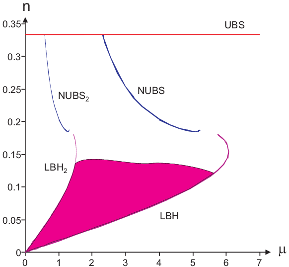
Refer to caption — Figure 1: Phase diagram for $d=5$ with $n$ versus $\mu$ for the two-black hole configurations spanning the area in between the single black hole (LBH) and two equal size black holes (LBH₂). Moreover, we have drawn the uniform black string phase (UBS), the non-uniform black string phase (NUBS) and its two-copied phase (NUBS₂).

From (4.10) and the inequality (5.1) we see that for a given mass $\mu$ we have a continuously infinite non-uniqueness of solutions with $k$ black holes. However, the non-uniqueness of solutions is even worse than this. If we consider a $k$ black hole solution it is described by $k$ parameters, as explained in Section 3.1. Thus, since the solutions with $k$ black holes span a two-dimensional area in the $(\mu,n)$ diagram we need $k-2$ extra parameters, beyond $\mu$ and $n$ , to point to a specific solution with $k$ black holes. Therefore, there is a continuous infinite non-uniqueness of solutions for certain points in the phase diagram, when $k\geq 3$ . Moreover, if we do not specify $k$ but instead consider all possible multi-black hole configurations, we have an infinite layer of solutions in the phase diagram, since one can always consider adding a small black hole to a given multi-black hole configuration.

Hence our results show a continuous non-uniqueness for solutions with fixed $M$ . Such non-uniqueness was also observed in Ref. [30] for bubble-black hole sequences, which are not spherically symmetric on $\mathbb{R}^{d-1}$ and lie in the region $\frac{1}{d-2}\leq n\leq d-2$ of the $(\mu,n)$ phase diagram. The multi-black hole configurations of this paper are therefore the first example of continuous non-uniqueness for solutions that are spherically symmetric on $\mathbb{R}^{d-1}$ .

Considering the phase diagram for the two black hole configurations depicted in Fig. 1, it is interesting to consider what happens when moving up in $n$ . One way to do this is to increase $\mu$ such that the ratios $\nu_{i}$ are fixed. In this case the two black holes are growing and eventually their horizons will meet. Thus, the natural question is then what happens when approaching this point. There seems to be two possibilities:

1)

When the horizons of the two black holes meet, their temperatures are not equal, and the solution will be singular in the meeting point.
2)

The temperatures of the two black holes will approach each other and when the two black holes meet they will merge into a new non-uniform black string phase different from both the original non-uniform black string phase emanating from the Gregory-Laflamme point, and the two-copied non-uniform black string phase.

We explore these scenarios further in Section 6.1. In Section 7 we discuss the possible implications for the Gregory-Laflamme instability if there should exist new non-uniform string phases.

Finally, we note that it is useful to give a rough estimate of the validity of the perturbative $k$ black hole solutions found in Section 2. For this purpose we can employ the estimate made for the single black hole solution in [17]. A lower estimate can be found by considering the $k$ copied phase, since we expect this to be the first solution for which the first order correction becomes invalid, as one increases $\mu$ . We therefore take the function $F(\rho,\theta)$ in (2.19) and consider when the contribution from the term with $\Lambda^{(i)}_{2}$ is equal to the one with $\Lambda^{(i)}$ . This happpens for $\rho^{2}\simeq 8\pi^{2}\zeta(d-2)/(k^{2}(d-1)(d-2)\zeta(d))$ . This can be used to get an upper bound for the Schwarzschild radius $k^{-1/(d-2)}\rho_{0}$ . Plugging that into $\mu$ in terms of $\rho_{0}$ , one obtains a rough upper bound on $\mu$ . For $k$ black holes, this means that the method is valid in the regime $\mu\ll\mu_{*}$ , with $\mu_{*}=30/k,9/k^{2},1.8/k^{3},0.2/k^{4},0.02/k^{5},0.002/k^{6}$ for $d=4,5,6,7,8,9$ . Therefore, for $k=2$ and $d=5$ we get that our perturbative solutions describing two black holes on the cylinder are valid for $\mu\ll 2.2$ , in accordance with Fig. 1. The values $\mu_{*}$ for $k=2$ black hole copies in $4\leq d\leq 9$ will be given in Table 1 in Section 6.1.

6 Further analysis of specific solutions

In this section we analyze in more detail the two simplest multi-black hole configurations, namely two- and three-black hole solutions. This serves as an illustration of the general solution and its physical properties, but will also provide us with further insights into the structure of the phase diagram discussed in the previous section, including the possibility of existence of new lumpy black holes in Kaluza-Klein spaces.

6.1 Two-black holes on the cylinder

We start by examining the case of the two-black hole solution, $i.e.$ we take a configuration of two black holes with mass fractions $\nu_{1}=\frac{1}{2}+\kappa$ and $\nu_{2}=\frac{1}{2}-\kappa$ , where $0\leq\kappa\leq 1/2$ so that by convention $M_{1}\geq M_{2}$ . Hence, $\kappa=0$ corresponds to a configuration with two black holes of equal mass, while the limiting case $\kappa=1/2$ is the single black hole solution. The locations of the black holes are chosen as $z_{1}^{*}=0$ and the location of the second black hole is denoted as $z_{2}^{*}$ . For the equilibrium configuration we clearly have $z_{2}^{*}=\pi$ so that the two black holes are on opposite points on the circle.

We first focus on the equilibrium configuration. To compute the various thermodynamic quantities we need $\Lambda^{(1,2)}$ defined in (2.20), which are given explicitly for the two-black hole case in Eq. (A.9). Furthermore, the expression for the sum $\sum_{i=1}^{2}\nu_{i}\Lambda^{(i)}$ is given in (A.10). The curve (4.9) in the phase diagram is thus given by

n(\mu;\kappa)=\frac{(d-2)\zeta(d-2)}{(d-1)\Omega_{d-1}}2^{d-4}\left[1-4\kappa^{2}\Big(1-2^{3-d}\Big)\right]\mu+{\cal{O}}(\mu^{2})\ .

(6.1)

Since the constant of proportionality is a monotonically increasing function of $\kappa$ one sees here explicitly that the inequality (5.1) at $k=2$ is obeyed, so that the slope in the $(\mu,n)$ phase diagram is bounded by that of a single black hole and two equal mass black holes.

From (4.11) and (A.9) we find the total entropy is given by

$\displaystyle S(\mu;\kappa)$	$\displaystyle=$	$\displaystyle S_{1}(\mu;\kappa)+S_{1}(\mu;-\kappa)\ ,$	(6.2)
$\displaystyle S_{1}(\mu;\kappa)$	$\displaystyle=$	$\displaystyle\frac{(2\pi)^{d-1}}{4\Omega_{d-1}^{\frac{1}{d-2}}(d-1)^{\frac{d-1}{d-2}}G_{\rm N}}\left[\Big(\frac{1}{2}+\kappa\Big)\,\mu\right]^{\frac{d-1}{d-2}}$	(6.3)
		$\displaystyle\times\left[1+\frac{\zeta(d-2)}{(d-2)\Omega_{d-1}}\left(2^{d-4}+2\kappa(1-\kappa)(1-2^{d-3})\right)\mu+{\cal{O}}(\mu^{2})\right]\ ,$	(6.3)

where we used that $S_{2}(\mu;\kappa)=S_{1}(\mu;-\kappa)$ . In particular, we find from this the corrected entropy of one black hole on a circle $S_{\rm 1BH}(\mu)\equiv S(\mu;1/2)$ and that of two equal mass black holes $S_{\rm 2eBH}(\mu)\equiv S(\mu;0)$ . We can now consider $S(\mu;\kappa)$ for fixed total (rescaled) mass $\mu$ as $\kappa$ ranges from 0 to $1/2$ . Physically, we expect that this is a monotonically increasing function of $\kappa$ since it should be entropically favored to have all the mass concentrated in one black hole, and the solution with two black holes is in an unstable equilibrium. As shown in Fig. 2, this is indeed the behavior we find when the mass of the system is not too large.

We can in fact use the physical criterion that $S(\mu;\kappa)$ be a monotonically increasing function of $\kappa$ to get an upper bound $\mu_{\rm c}$ on the mass, in order for our perturbative approach to be valid. By examining the function (6.2) in detail, we find that a condition that can be used to determine the critical mass is

\displaystyle\frac{\partial^{2}S(\mu=\mu_{\rm c};\kappa)}{\partial\kappa^{2}}{\biggr|}_{\kappa=0}=0\,,

(6.4)

where above we also used that $(\partial S(\mu,\kappa)/\partial\kappa)|_{\kappa=0}=0$ for all $\mu$ . Using the explicit expression (6.2) we have analyzed this equation for $4\leq d\leq 9$ and the results for $\mu_{\rm c}$ are listed in Table 1. A necessary condition for our method to be valid is thus $\mu\lesssim\mu_{\rm c}$ . We expect that for $\mu\ll\mu_{\rm c}$ our perturbative solution for the two-black hole configuration is valid. As illustrated in Table 1, this is a less restrictive bound than the one found in the end of Section 5 based on a less precise consideration.

$d$	$4$	$5$	$6$	$7$	$8$	$9$
$\mu_{\rm c}$	14.4	7.1	3.9	2.0	0.97	0.44
$\mu_{\rm*}$	15	2.2	0.2	$1\times 10^{-2}$	$8\times 10^{-4}$	$3\times 10^{-5}$
$\mu_{\rm GL}$	$3.52$	$2.31$	$1.74$	$1.19$	$0.79$	$0.55$

Table 1: The upper bound

\mu_{\rm c}

, imposed by entropy arguments, on the mass for the validity of the perturbative two-black hole results. For comparison the bound

\mu_{*}

(see end of Section 5) is shown along with the Gregory-Laflamme masses

\mu_{\rm GL}

(see e.g. [12]).

It is also useful to examine the temperatures of each of the black holes as we increase the mass. Clearly, for two black holes of unequal mass the zeroth order temperatures are different, and the system is not in thermal equilibrium. However, we can calculate the effect of the redshift on the ratio of temperatures, and examine whether this effect tends to equilibrate the black holes as we increase the total mass of the system. Using the first-order corrected temperatures (4.2) and the expressions (A.9) for $\Lambda^{(1,2)}$ one finds

\displaystyle\frac{T_{2}}{T_{1}}=\left(\frac{1+2\kappa}{1-2\kappa}\right)^{\frac{1}{d-2}}\left[1-\frac{4\,\kappa\,\zeta(d-2)}{(d-2)\Omega_{d-1}}(2^{d-3}-1)\mu+{\cal{O}}(\mu^{2})\right]\ ,

(6.5)

where we eliminated $\rho_{0}$ in favor of $\mu$ using (4.7), (4.9).

For two unequal mass black holes (with $M_{1}>M_{2}$ ) we have $0<\kappa<1/2$ so the pre-factor in (6.5) is greater than one. We now observe that as one increases the total mass $\mu$ the linear factor in $\mu$ will be smaller than one, causing the ratio $T_{2}/T_{1}$ to decrease towards one. We thus conclude that the first order redshifts combine in such a way that increasing the total mass of two unequal mass black holes causes the temperatures of the two black holes to approach each other. This indicates that it may be possible that in the full non-perturbative regime the temperatures converge to a common value at the merger.

Finally, we study the entropy of the more general configuration of two black holes without requiring the system to be in mechanical equilibrium. The total entropy $S(\mu;\kappa,z_{2}^{*})$ is obtained by using again (4.11) to compute the individual entropies $S_{1,2}$ , but now substituting the $z_{2}^{*}$ -dependent functions $\Lambda^{(1,2)}(z_{2}^{*})$ given in Eq. (A.8). We consider then a fixed total mass $\mu$ and mass distribution $\kappa$ , and vary the location $z_{2}^{*}$ of the second black hole where $0<z_{2}^{*}\leq\pi$ . Physically we expect that $S(\mu;\kappa,z_{2}^{*})$ is a monotonically decreasing function of $z_{2}^{*}$ , with minimal entropy when the black holes are farthest apart and maximal entropy when they have merged into a single black hole. This is indeed the case, as shown in Fig. 3.

We can view the decrease of $z_{2}^{*}$ as a time evolution process in which two black holes initially separated by a distance $\pi$ on the circle are perturbed and then collapse into a single black hole. As seen in Fig. 3 the total entropy increases during this process, but the entropy diverges as the distance between the black holes goes to zero. This is expected since fields diverge when we let the distance between sources go to zero in the point-particle limit, and indeed $\Lambda^{(1,2)}(z_{2}^{*})$ in (A.8) diverge as $z_{2}^{*}\rightarrow 0$ . However, for physical sources, the minimum distance of approach between the sources is given by their size. In our case, a good estimate for this critical distance is given by the horizon size of a $(d+1)$ -dimensional Schwarzschild (spherical) black hole with total mass $\mu$ , given by

\rho_{\rm s}\equiv 2\pi\left(\frac{\mu}{(d-1)\Omega_{d-1}}\right)^{\frac{1}{d-2}}\,.

(6.6)

On the other hand, we can compute the distance $z_{\rm c}$ at which the entropy curve $S(\mu;\kappa,z_{2}^{*})$ crosses the entropy $S_{\rm 1BH}(\mu)$ of a single black hole configuration (see Fig. 3), $i.e.$

S(\mu;\kappa,z_{\rm c})=S_{\rm 1BH}(\mu)\ .

(6.7)

Comparison of the two critical distances $\rho_{\rm s}$ and $z_{\rm c}$ now provides an important check on the validity of our perturbative method, since we expect these two numbers to be of the same order. As illustrated in Table 2 this match indeed occurs with $\rho_{\rm s}>z_{\rm c}$ , where for definiteness we have chosen $\kappa=0$ .

We thus conclude that also for non-equilibrium configurations the corrected thermodynamics leads to physically sensible results.

$d$	4				5				6
$\mu$	0.01	0.1	1	10	0.01	0.1	1	7	0.01	0.1	1	3
$z_{\rm c}$	$~0.055$	$~0.17$	$~0.52$	$~1.26$	$~0.25$	$~0.53$	$~1.13$	$~1.97$	$~0.54$	$~0.95$	$~1.68$	$~2.25$
$\rho_{\rm s}$	$~0.081$	$~0.26$	$~0.82$	$~2.58$	$~0.29$	$~0.62$	$~1.33$	$~2.54$	$~0.56$	$~1.00$	$~1.78$	$~2.34$

Table 2: Comparison of the two critical distances

z_{\rm c}

and

\rho_{\rm s}

in the case

\kappa=0

for some representative values of

d

and

\mu

(taken below the mass

\mu_{\rm c}

for which we can trust the perturbative results, see Table 1).

z_{\rm c}

is the minimum distance imposed by entropic considerations, as illustrated in Fig. 3, and

\rho_{\rm s}

is the size of a

(d+1)

-dimensional Schwarzschild black hole with mass

\mu

6.2 Three-black holes on the cylinder

In this subsection we discuss some features that can be addressed when we have three (or more) black holes, and we skip properties that are already present in the two-black hole configuration. In particular, by studying merges of two black holes we find evidence for new “lumpy” black hole configurations.

For definiteness, take a symmetric three-black hole configuration in equilibrium, located at the points $z_{1}^{*}=0$ , $z_{2}^{*}=\pi-y$ , and $z_{3}^{*}=\pi+y$ . We also adjust the masses $M_{i}=\nu_{i}M$ such that $\nu_{2}=\nu_{3}=\frac{1}{2}(1-\nu_{1})$ , $i.e.$ black hole 2 and 3 have equal mass. We now want to increase the total mass of the system while maintaining equilibrium. The black holes will thus increase in size and fill more and more of the free space in between them. The question we want to address is whether the two black holes 2 and 3 with the same mass will merge first, before merging with black hole 1, or whether black hole 1 will merge with the other two before 2 and 3 can merge.

As in the previous subsection, our answer to this question is limited by the fact that our formulae are strictly valid only for small black holes interacting via Newtonian gravity, while the black hole merging process we wish to consider is certainly one where the full nonlinearities of Einstein’s equations are important. However, we expect that with the available construction we can gain useful insights into the behavior of the system, so we proceed to examine this situation keeping in mind potential caveats.

The question above can be addressed by analyzing the ratio

\displaystyle X=\frac{\rho_{{\rm s}(1)}+\rho_{{\rm s}(2)}}{z_{12}}\frac{z_{23}}{\rho_{{\rm s}(2)}+\rho_{{\rm s}(3)}}\ ,

(6.8)

where $\rho_{{\rm s}(i)}$ is the Schwarzschild radius of the $i^{\rm th}$ black hole (defined as in (6.6)) and $z_{ij}$ is the distance between the $i^{\rm th}$ and $j^{\rm th}$ black holes. It is not difficult to see that this ratio is appropriate. Indeed, if black hole 1 joins 2 (and 3, by symmetry) first then at the point they merge one has $\frac{z_{12}}{\rho_{{\rm s}(1)}+\rho_{{\rm s}(2)}}=1$ and $\frac{z_{23}}{\rho_{{\rm s}(2)}+\rho_{{\rm s}(2)}}>1$ , so that $X>1$ . On the other hand, if 2 and 3 merge first then at one has $X<1$ at the merging point.

We can express the ratio $X$ defined in (6.8) as a function of the distance $y$ between black hole 1 and 2 (and 3) as follows. First one uses the relation $\rho_{{\rm s}(i)}\propto\left(\nu_{i}M\right)^{\frac{1}{d-2}}$ between the Schwarzschild radius and the black hole mass in $d+1$ dimensions along with the fact that $\nu_{2}=\nu_{3}$ , so that

\frac{\rho_{{\rm s}(1)}+\rho_{{\rm s}(2)}}{\rho_{{\rm s}(2)}+\rho_{{\rm s}(3)}}=\frac{1}{2}\left[1+\left(\frac{\nu_{1}}{\nu_{2}}\right)^{\frac{1}{d-2}}\right]=\frac{1}{2}\left[1+\left(\frac{V_{23}}{V_{12}}\right)^{\frac{1}{d-2}}\right]\ ,

(6.9)

where we used the equilibrium conditions (3.7) in the last step. Finally, we substitute the explicit expressions (3.4) for $V_{ij}$ where $z_{12}=z_{2}^{*}-z_{1}^{*}=\pi-y$ in $V_{12}$ and $z_{23}=z_{3}^{*}-z_{2}^{*}=2y$ in $V_{23}$ . Note that equilibrium requires $z_{23}<\pi$ , so we only consider $0<y<\pi/2$ . Equilibrium also demands that $\nu_{2}=\nu_{3}<\nu_{1}/2$ .

Collecting results, we use (6.9) to write the ratio in (6.8) as

	$\displaystyle X(y)$	$\displaystyle=$	$\displaystyle\frac{y}{\pi-y}{\biggl[}1+\left(\frac{\pi-y}{2y}\right)^{\frac{d-1}{d-2}}$		(6.10)
			$\displaystyle\qquad\quad\times\left(\frac{(2\pi)^{d-1}-(2y)^{d-1}\left[\zeta\left(d-1,1-\frac{y}{\pi}\right)-\zeta\left(d-1,1+\frac{y}{\pi}\right)\right]}{(2\pi)^{d-1}-(\pi-y)^{d-1}\left[\zeta\left(d-1,1-\frac{\pi-y}{2\pi}\right)-\zeta\left(d-1,1+\frac{\pi-y}{2\pi}\right)\right]}\right)^{\frac{1}{d-2}}{\biggr]}.$		(6.10)

We can understand (6.10) as follows. A given value of $y$ fixes the location and mass distribution of the system in equilibrium. Now let the total mass of the system increase. There is a critical value, call it $M_{23}$ , above which 2 and 3 are merged. Similarly above a critical value $M_{12}$ , 1 is merged with 2 (and 3). $X$ can then be expressed as the ratio $\left(M_{23}/M_{12}\right)^{\frac{1}{d-2}}$ . Thus, if $X<1$ , as we increase the total mass of the distribution, black hole 2 and 3 will merge before 1 joins them, and vice-versa.

A numerical analysis of (6.10) shows the following features, see Fig. 4. For $\frac{\pi}{3}<y<\frac{\pi}{2}$ , one has $X>1$ ; for $y_{*}<y<\frac{\pi}{3}$ , $X<1$ ; and for $0<y<y_{*}$ , $X>1$ again. Here, $y_{*}$ is a critical value that depends on the dimension of the spacetime. For example, for $d=4$ one has $y_{*}\sim\frac{\pi}{3.76}$ , while for $d=9$ one has $y_{*}\sim\frac{\pi}{55.56}$ . More generally, as $d$ grows $y_{*}$ decreases and the interval where $X<1$ grows.

To interpret these results first note that the case $y=\pi/2$ describes a two-black hole configuration that is the limiting case of the three-black hole configuration where $M_{1}\rightarrow 0$ , and we have two equal black holes each with mass $M/2$ located at $z=\pi/2$ and $z=3\pi/2$ . The case $y=\pi/3$ corresponds to a symmetric configuration with three equal black holes equally spaced along the circle. The case $y=0$ yields essentially the single-black hole limit of the three-black hole configuration where $M_{1}=M$ is centered at $z=0$ while $M_{2}=M_{3}\rightarrow 0$ . Therefore, as $y$ goes from $0$ to $\pi/2$ , the masses $M_{2}=M_{3}$ increase from $0$ up to $M/2$ , while $M_{1}$ decreases from $M$ to $0$ .

Keeping these features in mind, and that $\frac{\pi}{3}<y<\frac{\pi}{2}$ implies $z_{23}>z_{12}$ , it follows that as the total mass increases black hole 2 and 3 will merge with black hole 1 before they meet each other. We thus expect, as observed above, that $X>1$ for these values of $y$ and $X=1$ at the boundaries of the range. To understand the behavior of $X$ for $0<y<\frac{\pi}{3}$ it does not suffice to use purely geometrical arguments. Indeed, since $M_{1}>M_{2}$ in this branch, black hole 1 seems to approach 2 (and 3) faster than 2 and 3 approach each other, but since at the same time $z_{23}<z_{12}$ , we should use the numerical analysis of $X$ described above to determine what happens. This tells us that black hole 2 and 3 merge first, at least for $y_{*}<y<\frac{\pi}{3}$ where we found $X<1$ . However, for $y$ values smaller than $y_{*}$ the numerical results for $X$ are not reliable anymore, since in particular as $y\rightarrow 0$ we see that $X\rightarrow\infty$ which is due to the fact that our formulae are strictly valid in the point-particle limit where fields diverge when the distance between sources vanishes.

The results above suggest that it could be possible that after the merging of the two black holes (2 and 3) we end up with a“lumpy” black hole ( $i.e.$ a ‘peanut-like’ shaped black object) together with an ellipsoidal black hole (1). It is conceivable that such a configuration would be a new static black hole solution in asymptotically $\mathcal{M}^{d}\times S^{1}$ spacetimes. Generally if two black holes were to merge in this way, we expect that the resulting configuration would be singular. The singularity would arise if the surface gravities or temperatures of the two black holes differed, following standard results of [36, 37]. In the above construction, however, we chose $M_{2}=M_{3}$ to make the surface gravities identical in the merger.

To discuss this further, note first of all that it is still true that the area of one spherical black hole of given mass is bigger than the sum of the areas of two isolated black holes with the same total mass. Nevertheless, the following argument suggests the possibility of lumpy objects for $d\geq 4$ . In general dimension $d+1$ , the horizon radius of a Schwarzschild black hole scales as $\rho_{{\rm s}}\sim M^{\frac{1}{d-2}}$ , so starting from two black holes with $\rho_{{\rm s}(1,2)}\propto M_{1,2}^{\frac{1}{d-2}}$ we have at the merging point a total radius $\rho_{{\rm s}(1)}+\rho_{{\rm s}(2)}\propto M_{1}^{\frac{1}{d-2}}+M_{2}^{\frac{1}{d-2}}$ . On the other hand a single black hole with mass $M_{1}+M_{2}$ has a radius $\rho_{{\rm s}(12)}\propto(M_{1}+M_{2})^{\frac{1}{d-2}}$ . In four dimensions ( $d=3$ ) this scales the same way as the total radius of the merged object so we expect the formation of a spherical black hole [38]. However, for $d\geq 4$ the power in the exponent is less than one so that $\rho_{{\rm s}(1)}+\rho_{{\rm s}(2)}>\rho_{{\rm s}(12)}$ . Hence we should expect that the resulting merger configuration will not be surrounded by a spherical horizon, as would occur for $d=3$ .

As a consequence, it seems that for $d\geq 4$ this analysis does not rule out the possibility of having a configuration of a lumpy black object with “centers” at $z=\pi\pm y$ kept in an unstable equilibrium by a black hole at $z=0$ (and the respective copies). Note also that the argument above suggests that the higher the dimension, the more likely it is that lumpy black holes will exist. Finally, we emphasize that the above analysis should be read within the earlier-mentioned limitations of our construction.

Note that in asymptotically flat space new stationary black holes with similar ‘rippled’ horizons of spherical topology have been argued to exist in Ref. [39] by considering ultraspinning Myers-Perry black holes in dimensions greater than six. While in that case the ripples are supported by the angular momentum $J$ in our case they are supported by the external stress of the other (ellipsoidal) black hole. It would be interesting to generalize the analysis above to configurations with more bumps, for example taking a symmetric four-black hole configuration with $M_{2}=M_{3}=M_{4}$ .

7 Conclusions and outlook

7.1 Summary

In this paper we constructed solutions of the vacuum Einstein equations describing multi-black hole configurations on the cylinder $\mathbb{R}^{d-1}\times S^{1}$ with $d\geq 4$ , in the limit of small total mass, or, equivalently, in the limit of a large cylinder. These solutions generalize the analytic solutions found for the single black hole on the cylinder [17, 18, 19, 20, 21]. Furthermore, they generalize the so-called copies of the single black hole solutions corresponding to having equal mass black holes distributed equidistantly around the cylinder [28, 29]. The new solutions are valid to first order in the total mass, and are constructed using the technique of [17] based on an ansatz for the metric found in [16].

Using the first-order corrected metrics for the multi-black hole configurations we have studied their thermodynamics. Included in this is one of the central results of this paper: The relative tension (binding energy) $n$ as a function of the total (rescaled) mass $\mu$ , as given by Eq. (4.9). Using this, we have shown how the solutions appear in the $(\mu,n)$ phase diagram [12, 29], together with the other known solutions that asymptote to $\mathcal{M}^{d}\times S^{1}$ . We observed that a multi-black hole configuration with $k$ black holes has $k$ independent parameters. This implies a continuous non-uniqueness in the $(\mu,n)$ phase diagram (or for a given mass), much like the one observed for bubble-black hole sequences [30].

The multi-black hole configurations have to be in mechanical equilibrium in order to have a static solution. We have identified where this requirement appears in the construction of the solution, and we have furthermore examined how to build such equilibrium configurations. Moreover, we have described a general copying mechanism that enables us to build new equilibrium configurations by copying any given equilibrium configuration a number of times around the cylinder.

Finally, we examined in detail configurations with two and three black holes. For two black holes we verified the expectation that one maximizes the entropy by transferring all the mass to one of the black holes, and also that if the two black holes are not in mechanical equilibrium then the entropy is increasing as the black holes become closer to each other. These two facts are both in accordance with the general argument that the multi-black hole configurations are in an unstable equilibrium and generic perturbations of one of the positions will result in that all the black holes merge together in a single black hole on the cylinder. For the three black hole solution we examined and found preliminary evidence for the hypothesis that for certain three-black hole configurations two of the black holes can merge into a lumpy black hole, where the non-uniformities are supported by the gravitational stresses imposed by an external field.

From the first-order corrected temperatures one can show that the multi-black hole configuration are in general not in thermal equilibrium. The only configurations that are in thermal equilibrium to this order are the copies of the single-black hole solution studied previously [28, 29, 17]. As a further comment we note that Hawking radiation will seed the mechanical instabilities of the multi-black hole configurations. The reason for this is that in a generic configuration the black holes have different rates of energy loss and hence the mass ratios required for mechanical equilibrium are not maintained. This happens even in special configurations, e.g. when the temperatures are equal, because the thermal radiation is only statistically uniform. Hence asymmetries in the real time emission process will introduce disturbances driving these special configurations away from their equilibrium positions.

7.2 Discussion of the phase structure

We now examine the appearance of our new multi-black hole phases in connection to the known phases of black holes and black strings on the cylinder (See [1, 2, 3] for reviews). In particular, as mentioned in the introduction there is the well-known phase of the uniform black string (UBS) as well as the non-uniform black string (NUBS), emanating from the uniform phase at the Gregory-Laflamme point $\mu_{\rm GL}$ . Recently, numerical investigations [11, 13, 14, 15, 22, 23, 24] confirmed the prediction [25] that the non-uniform phase connects via a horizon topology changing phase transition [25, 26, 27, 15] to the phase of a single localized black hole (LBH) (see Fig. 1). This point is generally referred to as the merger point.

Moreover, as reviewed in Section 3, for any solution that falls into the $SO(d-1)$ -symmetric ansatz (2.1) of Ref. [16], one can obtain a copied solution [28, 29, 17] by changing the periodicity of the circle from $L$ to $kL$ with $k$ an integer. As mentioned above, this includes the localized black hole phase, from which one generates in this way the multi-black hole solutions with $k$ equal mass black holes, which we denote by LBH_k. It also includes the non-uniform black string phase, from which we generate copies which we denote by NUBS_k, emerging from the uniform phase at critical mass $\mu_{\rm GL}/k^{d-3}$ . This thus means that the LBH_k phase will connect to the NUBS_k phase via a horizon topology changing phase transition at the $k$ -copied merger point (see Fig. 1 for $k=2$ ).

We now turn to the question posed in Section 5: Where do all the new multi-black hole phases end in the phase diagram? For definiteness, let us consider again configurations with two black holes. The LBH and NUBS phases are connected via the topology-changing merger point, and likewise the LBH₂ and NUBS₂ phases are connected via the 2-copied merger point. As explained in Section 5 all two-black hole configurations with unequal mass lie (at least for small masses) in between these two limiting phases and it is not clear where these phases will end up in the phase diagram. Two scenarios where given in Section 5, and we now examine in more detail the possibility of the second scenario, namely that the black holes merge into a new non-uniform string. Recall that this would require the temperatures of the black holes to approach each other at the merger point.

First of all, we have seen in Section 6.1 that our first order result for the temperatures shows that the temperatures of the two black holes are redshifted in such a way that they tend to approach each other. This lends credibility to the possibility that indeed in the full non-perturbative regime the temperatures may converge to a common value at the merger. If this is the case, it seems to suggest that there would exist new non-uniform black strings beyond the NUBS_k phases, to which the unequal mass black hole configurations could connect via new merger points.¹⁰¹⁰ 10 Note that the original argument by Kol [25, 1] for the merger transition of the LBH and NUBS phases was based on Morse theory, which loosely speaking implies that the LBH phase cannot end in “nothing”.

If smooth mergers do occur for different size black hole configurations, an important question to consider is whether this a generic feature, or if it only happens for particular configurations. Consider for the example the case of two black holes, for which we have two free parameters namely the total mass and the ratio of the individual masses. Equating their temperatures fixes the mass ratio as a function of the total mass (see Eq. (6.5)). Similarly achieving a merger of the black holes also fixes the ratio with another function of the total mass. If we imagine these two functions of the mass to be independent, it follows that we only expect these two functions to intersect at discrete points in the space of parameters defining the configuration. On the other hand, if these two functions are not independent, due to the interrelation between geometry and energy in General Relativity, one can instead imagine that the two functions always intersect, so that the smooth mergers are a generic feature.

As discussed above, smooth mergers for different size black hole configurations suggest that new non-uniform black string phases exist. If this is the case, there are certain constraints on such new phases from general arguments. Firstly, it is clearly not possible that there are non-uniform black strings emerging from the uniform black string in the range $\mu_{\rm GL}/2^{d-3}<\mu<\mu_{\rm GL}$ [8]. Also, it does not seem possible that one can have other branches than the known ones coming out of the Gregory-Laflamme point (or its $k$ -copies) of the uniform black string given the higher-order perturbative analysis of Ref. [10]. Secondly, it is impossible to (locally) have a continuum of non-uniform black string solutions in the phase diagram. To prove this assertion imagine that there is a two-dimensional continuous parameter space of solutions and consider two points, say $A$ and $B$ , in this continuum. It follows from the continuity that one can always connect these two points by two different paths of solutions. Imagine now that the two-dimensional space of solutions projects into a two-dimensional region in the $(\mu,n)$ phase diagram. If we then furthermore take the paths so that $n$ in path 1 is greater than $n$ in path 2, then we get an contradiction when using the Intersection Rule of Ref. [12]. This is because $\delta(S_{1}/S_{2})=(n_{1}-n_{2})M\delta M/((d-1)T_{1}T_{2}S_{2}^{2})$ where the indices on the quantities refer to the paths. Since $n_{1}>n_{2}$ , the right hand side is strictly positive. Thus, the ratio $S_{1}/S_{2}$ in point B should be greater than 1, but that is not possible since the two paths should go to the same solution. We thus conclude that a locally continuous space of solutions is impossible¹¹¹¹ 11 Note that implicit in the above argument is the assumption that there is only one connected horizon with a given temperature. Thus, the fact that multi-black hole configurations cover a continuous region in the phase diagram is not a contradiction because they contain disconnected horizons typically at different temperatures., except in the very special case where the continuous space of solutions projects onto a one-dimensional subspace in the $(\mu,n)$ phase diagram. This provides a further argument that smooth mergers would only occur at discrete points, because there could only be a discrete set of non-uniform string solutions to which the the merging black holes could connect.

Given these two constraints, there is still the possibility that new non-uniform black strings may exist. Namely, it is conceivable that the NUBS_k phases ( $k\geq 1$ ) develop their own zero modes as one moves away a finite distance away from the GL point (or its $k$ -copies). This is a non-perturbative effect that would not show up in the perturbative analysis of Gubser. These zero-modes on the non-uniform black string would in fact imply that they have some region in which they are respectively classically unstable or stable, just as for the uniform black string. Such a bifurcation of new non-uniform strings from the presently known ones would also be discrete and thereby evade the second restriction presented above. Furthermore, in this scenario one could imagine a fractal structure of further bifurcations into new non-uniform strings, all of which eventually end up in a particular multi-black hole configuration. If true, this would fit well with the smooth mergers of different size black hole configurations occurring only at a discrete points in the space of configurations. It would be very interesting to explore this possibility further.

Another point that we already alluded to in Section 5 is that we do not expect the phases of two black hole configurations to stay in between the LBH and LBH₂ curves in the $(\mu,n)$ phase diagram (and similarly for multi-black hole configurations with more than two black holes). To see this consider the LBH curve in Fig. 1. This curve has a point at which $\mu$ is maximal, occurring well before the merger point. Beginning with this maximal mass single-black hole configuration we can add a tiny black hole on the opposite side of the circle and reach a two-black hole configuration with greater mass than the original configuration. This clearly implies that the two-black hole configurations can extend outside the wedge bounded by the LBH and LBH₂ curves. In fact, one can similarly argue by starting from the extremal point on the LBH₂ curve that by removing a tiny mass from one of the two black holes, one can reach a two-black hole configuration to the left of this curve. Another interesting example comes from adding a pair of tiny black holes to any LBH₂ configuration to produce a four-black hole configuration in its neighborhood in the phase diagram, very far away from the wedge enclosed by the LBH₃ and LBH₄ curves. The above reasoning can be extended by imagining further additions of tiny masses, in more complicated starting configurations, leading to a intricate pattern of crossings of lines in the $(\mu,n)$ phase diagram.

We have also presented evidence in this paper for the possibility of a new class of static lumpy black holes in Kaluza-Klein space. Again, it would be interesting to study this further, and examine how these in turn might connect to new non-uniform phases.

7.3 A fluid analogy

It is also interesting, though more speculative, to consider the appearance of the multi-black hole configurations in relation to an analogue model for the Gregory-Laflamme (GL) instability, recently proposed in Ref. [40]. There it was pointed out that the GL instability of a black string has a natural analogue description in terms of the Rayleigh-Plateau (RP) instability of a fluid cylinder. It turns out that many known properties of the gravitational instability have an analogous manifestation in the fluid model. These include the behavior of threshold mode with $d$ , dispersion relations, the existence of critical dimensions and the initial stages of the time evolution¹²¹² 12 Recently, another feature of these instabilities has been matched. If rotation is added to the fluid the strength of the fluid instability increases because the centrifugal force is bigger in a crest than in a trough of the configuration. On the gravity side it was found in Ref. [41] that rotating black strings, even for large rotation, are indeed also unstable to the GL instability. (see Refs. [40, 42, 43] for details).

Since our reasoning below relies on the time evolution of the system and its endpoint, it is worth mentioning that the full time evolution of the RP instability is well known (both numerically and experimentally, see Refs. [44, 45, 46, 47] for details). On the gravity side only the initial stages of the GL instability has been numerically studied so far [48]. Comparing with the fluid system there is an interesting match between the initial stage of the evolution in the two systems. Starting from a single sinusoidal perturbation both develop an almost cylindrical thread or neck in between the two half rounded boundary regions. This can be confirmed by comparing Fig. 1 of [46] (which describes the full RP evolution) and Fig. 2 of [48] (that describes the initial stage of the GL evolution).

One should be cautious when applying the analogue model, especially in what concerns the evolution of the systems. The reason is that the analogy is partly based on the similarity between the first law of black hole thermodynamics and the fluid relation $dE=TdA$ where $E$ is the potential energy associated with surface tension (free energy), $T$ the effective surface tension and $A$ the surface area of the fluid. This means that both systems tend to extremize the area. However, on the gravity side we know that a black object evolves such that its horizon area never decreases, whereas a fluid evolves toward a configuration with smaller area, since this decreases its potential energy. Despite these reversed dynamical features, it is worthwhile to notice that just like a multi-black hole system will maximize its entropy by merging into one single black hole containing all the mass, so will an array of fluid droplets merge into a single drop in order to minimize its surface area at fixed volume.

Having alerted the reader to these caveats, we proceed with the analogy in hand, considering the time evolution of the fluid in further detail. A representative study of particular interest for our purposes was carried out in [46]. The main conclusion is that if we start with a single sinusoidal perturbation in a cylindrical liquid bridge, the higher harmonics generated by non-linear effects are responsible for the development of a long neck that breaks¹³¹³ 13 Note that at the pinch-off there is another similarity that characterizes both instabilities. On the gravity side, one would need to use quantum gravity when the pinch-off region reaches the Planck scale and General Relativity is no longer valid. Likewise, close to breakup of the fluid, when the radius of the liquid bridge is of molecular size, the (continuum) hydrodynamic theory is no longer a good approximation and simulations of the molecular dynamics are required. in a self-similar process [46, 44, 45]. We end up with an array of satellite drops with different sizes. Hence, if the correspondence indeed extends to the full evolution, the multi-black holes would be the natural gravity analogues of the main drop and satellite droplets array observed in the fluid analysis.

Furthermore the analogue model would thus argue in favor of the scenario in which the neutral black string will pinch off. Moreover, the multi-black hole configurations constructed in this paper would play an important role in the intermediate stages of the GL instability. It would be interesting to examine this application of the analogue fluid model and its consequences more closely.

7.4 Outlook

The study of Kaluza-Klein black holes and their high degree of non-uniqueness can be viewed in the broader context of studying black objects in higher dimensional gravity. Here, research in the last years has revealed that also in asymptotically flat space a very rich phase structure of stationary black objects is expected. In particular, in five-dimensional Einstein gravity there exists, beyond the rotating Myers-Perry black hole, a black ring solution [49] (see [50] for a review). Recently further new stationary solutions, called ‘black Saturns’ [32, 33], have been constructed explicitly in five-dimensional gravity. These solutions, consisting of a spherical black hole with black rings around it, are similar to the multi-black hole configurations, in that the generic solution is not in thermal equilibrium, with different temperatures for each connected component of the event horizon. Furthermore, one may compare the configurations with highest entropy in the two systems. It was shown in Ref. [34] that the maximal entropy configuration for fixed mass and angular momentum consists of a central, close to static, black hole and a very thin black ring around it. For any value of the angular momentum, the upper bound on the entropy is then equal to the entropy of a static black hole of the same total mass. These maximal entropy black Saturns are not in thermal equilibrium. In some sense the same features are observed for multi-black hole configurations. If we restrict to the case of two black holes, the highest entropy configuration (see Section 6.1) is that of an infinitesimally small black hole together with a large black hole, $i.e.$ far away from thermal equilibrium. The entropy of that configuration is bounded from above by that of a single black hole of the same mass.

It is also worth emphasizing that the solution technique employed in this paper can be applied to other black hole systems where one lacks the symmetries or other insights to construct exact solutions. The general idea is to identify a suitable perturbation parameter of the putative solution, and follow similar steps as outlined in Section 2.

Another open direction to pursue is to apply numerical techniques to extend the construction of multi-black hole configurations into the non-perturbative regime, as was successfully done for a single black hole on a cylinder in five and six dimensions [22, 23, 24]. Such an analysis could confirm whether indeed there are multi-black hole configurations for which the temperatures converge when approaching the merger points as one increases the mass, as was discussed in Section 6.1. Furthermore, it is possible that in this way one could confirm the existence of the lumpy black holes conjectured in Section 6.2, where we recall that these are most likely for higher dimensions.

A further, but technically complicated, direction to pursue is to extend the solutions of this paper to the next, $i.e.$ second, order. For the case of a single black hole in five dimensions, the second order correction to the metric and thermodynamics have been studied in [20]. More generally, the second order correction to the thermodynamics was obtained in Ref. [21] for all $d$ using an effective field theory formalism in which the structure of the black hole is encoded in the coefficients of operators in an effective worldline Lagrangian. It would be interesting to obtain the second-order corrected metric and thermodynamics for the multi-black hole case considered in this paper.

There are also potential applications related to string theory and gauge theory. It is known that the phases of Kaluza-Klein black holes are related via a boost/U-duality map [51] (see also [52, 53]) to phases of non- and near-extremal branes on a transverse circle, appearing as solutions in type II string theory or M-theory. Via the gauge/gravity correspondence [54, 55] this has implications for the phase structure of the dual non-gravitational theories at finite temperature. For instance, it is possible to obtain in this way non-trivial predictions [53, 51, 56] about the strong coupling dynamics of supersymmetric Yang-Mills theories on compact spaces and of the thermal behavior of little string theory.

As an important example, Ref. [53] considered finite temperature two-dimensional supersymmetric Yang-Mills on a spatial circle, which by the boost/U-duality map is related to the phase structure of Kaluza-Klein black holes in ten dimensions. The corresponding phase structure that is present at strong coupling in the two-dimensional Yang-Mills theory on the torus $S^{1}_{\beta}\times S^{1}$ was then qualitatively matched to the phase structure in the weakly coupled gauge theory. In particular, it was found in [53] that the eigenvalue distribution of the spatial Wilson loop distinguishes between the three different phases seen at strong coupling: The uniform phase corresponds to a uniform eigenvalue distribution, the non-uniform phase corresponds to a non-uniform eigenvalue distribution and the localized phase maps to a gapped eigenvalue distribution. It would be interesting to see if there are also multiply gapped eigenvalue distributions (see e.g. Ref. [57]), corresponding to the localized phase of multi-black holes found in this paper. While those would probably be unstable as mentioned above, they may still appear as unstable saddle points.

Finally, we remark on an open direction that is related to microscopic calculations of the entropy of black holes. In Ref. [58] (see [59] for a short summary) the boost/U-duality map of [51] was extended to the case of branes with more than one charge. One of the results is that by starting with neutral Kaluza-Klein black holes in five dimensions one can generate five-dimensional three-charge black holes on a circle, obtained from corresponding three-charge brane configurations in type II/M-theory via compactification. In particular, when one applies this map to a single neutral localized black hole one obtains a three-charge black hole localized on the transverse circle. For this case, it was shown that in a partial extremal limit with two charges sent to infinity and one finite, the first correction to the finite entropy is in agreement with the microscopic entropy.¹⁴¹⁴ 14 The entropy matching for the single three-charge black hole case considered in [58] was extended in Ref. [60] to second order. By applying the map to the multi-black hole solutions of this paper one will generate three-charge multi-black holes on a circle. The results of Section 4 can then be used to compute the first correction to the finite entropy of these three-charge multi-black hole configurations, and it would be interesting to then derive these expressions from a microscopic calculation as well. Furthermore, in Ref. [60] a simple microscopic model was proposed that reproduces most of the features of the phase diagram of three-charge black holes on a circle, including the new non-uniform phase. It would be interesting to see if this model can also account for the corresponding localized three-charge multi-black hole solutions.

Acknowledgements

We thank Henriette Elvang, Roberto Emparan, Gary Horowitz, Veronika Hubeny, Barak Kol, Don Marolf, Mukund Rangamani, Evgeny Sorkin and Toby Wiseman for useful discussions. The authors would like to thank the KITP for hospitality during the program “Scanning new horizons: GR beyond 4 dimensions”, where this work was started. The authors would also like to thank the organizers of the workshops ”Einstein’s Gravity in Higher Dimensions” Jerusalem Feb. 18-22, 2007, and ”Pre-strings 2007” Granada June 18-22, 2007 where part of this work was done. OD acknowledges the hospitality of the Perimeter Institute during early stages of this work. This work was partially funded by Fundação para a Ciência e Tecnologia (FCT, Portugal) through project PTDC/FIS/64175/2006. OD acknowledges financial support provided by the European Community through the Intra-European Marie Curie contract MEIF-CT-2006-038924. The work of TH and NO is partially supported by the European Community’s Human Potential Programme under contract MRTN-CT-2004-005104 ‘Constituents, fundamental forces and symmetries of the universe’. TH would like to thank the Carlsberg Foundation for support. Research at the Perimeter Institute is supported in part by the Government of Canada through NSERC and by the Province of Ontario through MRI. RCM also acknowledges funding from an NSERC Discovery grant and the Canadian Institute for Advanced Research. Research at the KITP was supported in part by the NSF under Grant No. PHY05-51164.

Appendix A Data for two unequal mass black holes

In this appendix we give some useful explicit expressions for the quantities that are involved in the construction of the two-black hole configuration, further discussed in Section 6.1.

The mass fractions of the two black holes are taken as $\nu_{1}=\frac{1}{2}+\kappa$ , $\nu_{2}=\frac{1}{2}-\kappa$ and the equilibrium configuration is chosen such that the first black hole at $z_{1}^{*}=0$ and the second at $z_{2}^{*}=\pi$ , $i.e.$ at opposite points on the circle. The function (2.7) entering the Newtonian potential is then given by

F(r,z)=2^{d-3}{\cal{F}}(2r,2z)+2^{d-2}\kappa\ \hat{\cal{F}}(2r,2z)\,,

(A.1)

where we have defined

{\cal{F}}(r,z)\equiv\sum_{m=-\infty}^{\infty}\frac{1}{[r^{2}+(z-2\pi m)^{2}]^{\frac{d-2}{2}}}\,,\ \ \hat{\cal{F}}(r,z)\equiv\sum_{m=-\infty}^{\infty}\frac{(-1)^{m}}{[r^{2}+(z-2\pi m)^{2}]^{\frac{d-2}{2}}}\,.

(A.2)

The function ${\cal{F}}(r,z)$ is identical to the one entering the Newtonian potential for the single black hole case, and details can be found in Appendix B of [16]. Using Poisson resummation the large $r$ expansions of the two functions in (A.2) are obtained as

\displaystyle{\cal{F}}(r,z)=\frac{k_{d}}{r^{d-3}}{\biggl(}1+2\sum_{m=1}^{\infty}h(mr)\cos(mz){\biggr)}\,,

(A.3)

\hat{\cal{F}}(r,z)=\frac{2k_{d}}{r^{d-3}}\sum_{m=0}^{\infty}h([m+1/2]r)\cos([m+1/2]z)\,,

(A.4)

where $k_{d}$ and $h(x)$ are defined in (2.9), (2.10) respectively.

Note that for even $d$ , the relevant Bessel function takes the form of a polynomial of finite degree. This allows to write explicit expressions for ${\cal F}(r,z)$ and $\hat{\cal F}(r,z)$ (and similarly for $v(r,z)$ in (2.14)). For example, for $d=4$ one has

\displaystyle{\cal{F}}(r,z)=\frac{1}{2r}\frac{\sinh r}{\cosh r-\cos z}\,,\qquad\hat{\cal{F}}(r,z)=\frac{1}{r}\frac{\sinh(r/2)\cos(z/2)}{\cosh r-\cos z}\,,\qquad{\rm for}\>\>d=4\,.

(A.5)

For $d=6$ one has

$\displaystyle{\cal{F}}(r,z)$	$\displaystyle=$	$\displaystyle\frac{1}{4r^{3}}\frac{\sinh r}{\cosh r-\cos z}+\frac{1}{2r^{2}}\frac{\sinh^{2}(r/2)\cos^{2}(z/2)-\cosh^{2}(r/2)\sin^{2}(z/2)}{(\cosh r-\cos z)^{2}}\,,$
$\displaystyle\hat{\cal{F}}(r,z)$	$\displaystyle=$	$\displaystyle\frac{1}{2r^{3}}\frac{\sinh(r/2)\cos(z/2)}{\cosh r-\cos z}+\frac{1}{8r^{2}}\frac{\sinh^{2}(r/4)\cos^{2}(z/4)-\cosh^{2}(r/4)\sin^{2}(z/4)}{[\cosh(r/2)-\cos(z/2)]^{2}}$	(A.6)
		$\displaystyle+\frac{1}{8r^{2}}\frac{\cosh^{2}(r/4)\cos^{2}(z/4)-\sinh^{2}(r/4)\sin^{2}(z/4)}{[\cosh(r/2)+\cos(z/2)]^{2}}\,,\qquad{\rm for}\>\>d=6\,.$	(A.6)

For the small $\rho$ expansion, we first present the results for general location $z_{2}^{*}$ of the second black hole, restricting to the equilibrium configuration $z_{2}^{*}=\pi$ at the end. In the region near the first or second black hole respectively, we have from (2.19) the expansions

F(r,z)\simeq\frac{\frac{1}{2}+\kappa}{\rho^{d-2}}+\Lambda^{(1)}\,,\ \ \qquad F(r,z)\simeq\frac{\frac{1}{2}-\kappa}{\rho^{d-2}}+\Lambda^{(2)}\,,

(A.7)

where $\Lambda^{(1,2)}$ are computed from (2.20)

	$\displaystyle\Lambda^{(1)}=\frac{(\frac{1}{2}+\kappa)2\zeta(d-2)}{(2\pi)^{d-2}}+\frac{\frac{1}{2}-\kappa}{(z_{2}^{})^{d-2}}+\frac{\frac{1}{2}-\kappa}{(2\pi)^{d-2}}\left[\zeta\left(d-2,1+\frac{z_{2}^{}}{2\pi}\right)+\zeta\left(d-2,1-\frac{z_{2}^{*}}{2\pi}\right)\right]\,,$
	$\displaystyle\Lambda^{(2)}=\frac{(\frac{1}{2}-\kappa)2\zeta(d-2)}{(2\pi)^{d-2}}+\frac{\frac{1}{2}+\kappa}{(2\pi-z_{2}^{})^{d-2}}+\frac{\frac{1}{2}+\kappa}{(2\pi)^{d-2}}\left[\zeta\left(d-2,2-\frac{z_{2}^{}}{2\pi}\right)+\zeta\left(d-2,\frac{z_{2}^{*}}{2\pi}\right)\right]\,,$
			(A.8)

and we recall the definitions (2.23), (2.24). In particular, for the equilibrium configuration $z_{2}^{*}=\pi$ these expressions reduce to

\Lambda^{(1)}=[2^{d-3}+2\kappa(1-2^{d-3})]\frac{2\zeta(d-2)}{(2\pi)^{d-2}}\,,\ \ \quad\Lambda^{(2)}=[2^{d-3}-2\kappa(1-2^{d-3})]\frac{2\zeta(d-2)}{(2\pi)^{d-2}}\,.

(A.9)

Note that for $\kappa=1/2$ , the expression for $\Lambda^{(1)}$ reduces to the correct result for a single black hole. Finally, we record the sum

\displaystyle\sum_{i=1}^{2}\nu_{i}\Lambda^{(i)}=2^{d-3}\,\frac{2\zeta(d-2)}{(2\pi)^{d-2}}\left[1+2^{5-d}\left(1-2^{d-3}\right)\kappa^{2}\right],

(A.10)

which is used in the text to compute various thermodynamic quantities.

References

[1] B. Kol, Phys. Rept. 422 (2006) 119–165, hep-th/0411240.
[2] T. Harmark and N. A. Obers, hep-th/0503020.
[3] T. Harmark, V. Niarchos, and N. A. Obers, Class. Quant. Grav. 24 (2007) R1–R90, hep-th/0701022.
[4] R. C. Myers, Phys. Rev. D35 (1987) 455.
[5] A. R. Bogojevic and L. Perivolaropoulos, Mod. Phys. Lett. A6 (1991) 369–376.
[6] D. Korotkin and H. Nicolai, gr-qc/9403029.
[7] A. V. Frolov and V. P. Frolov, Phys. Rev. D67 (2003) 124025, hep-th/0302085.
[8] R. Gregory and R. Laflamme, Phys. Rev. Lett. 70 (1993) 2837–2840, hep-th/9301052.
[9] R. Gregory and R. Laflamme, Nucl. Phys. B428 (1994) 399–434, hep-th/9404071.
[10] S. S. Gubser, Class. Quant. Grav. 19 (2002) 4825–4844, hep-th/0110193.
[11] T. Wiseman, Class. Quant. Grav. 20 (2003) 1137–1176, hep-th/0209051.
[12] T. Harmark and N. A. Obers, Class. Quantum Grav. 21 (2004) 1709–1724, hep-th/0309116.
[13] E. Sorkin, Phys. Rev. Lett. 93 (2004) 031601, hep-th/0402216.
[14] B. Kleihaus, J. Kunz, and E. Radu, JHEP 06 (2006) 016, hep-th/0603119.
[15] E. Sorkin, Phys. Rev. D74 (2006) 104027, gr-qc/0608115.
[16] T. Harmark and N. A. Obers, JHEP 05 (2002) 032, hep-th/0204047.
[17] T. Harmark, Phys. Rev. D69 (2004) 104015, hep-th/0310259.
[18] D. Gorbonos and B. Kol, JHEP 06 (2004) 053, hep-th/0406002.
[19] D. Gorbonos and B. Kol, Class. Quant. Grav. 22 (2005) 3935–3960, hep-th/0505009.
[20] D. Karasik, C. Sahabandu, P. Suranyi, and L. C. R. Wijewardhana, Phys. Rev. D71 (2005) 024024, hep-th/0410078.
[21] Y.-Z. Chu, W. D. Goldberger, and I. Z. Rothstein, JHEP 03 (2006) 013, hep-th/0602016.
[22] E. Sorkin, B. Kol, and T. Piran, Phys. Rev. D69 (2004) 064032, hep-th/0310096.
[23] H. Kudoh and T. Wiseman, Prog. Theor. Phys. 111 (2004) 475–507, hep-th/0310104.
[24] H. Kudoh and T. Wiseman, Phys. Rev. Lett. 94 (2005) 161102, hep-th/0409111.
[25] B. Kol, hep-th/0206220.
[26] T. Wiseman, Class. Quant. Grav. 20 (2003) 1177–1186, hep-th/0211028.
[27] B. Kol and T. Wiseman, Class. Quant. Grav. 20 (2003) 3493–3504, hep-th/0304070.
[28] G. T. Horowitz, hep-th/0205069.
[29] T. Harmark and N. A. Obers, Nucl. Phys. B684 (2004) 183–208, hep-th/0309230.
[30] H. Elvang, T. Harmark, and N. A. Obers, JHEP 01 (2005) 003, hep-th/0407050.
[31] R. Emparan, JHEP 03 (2004) 064, hep-th/0402149.
[32] H. Elvang and P. Figueras, hep-th/0701035.
[33] H. Iguchi and T. Mishima, Phys. Rev. D75 (2007) 064018, hep-th/0701043.
[34] H. Elvang, R. Emparan, and P. Figueras, hep-th/0702111.
[35] M. Abramowitz and A. Stegun, Handbook of mathematical functions, (Dover Publications, New York, 1970).
[36] J. M. Bardeen, B. Carter and S. W. Hawking, Commun. Math. Phys. 31 (1973) 161.
[37] I. Racz, and R. M. Wald, Class. Quant. Grav. 9 (1992) 2643–2656.
[38] K. S. Thorne, in Magic without Magic: John Archibald Wheeler, edited by J.Klauder (Freeman, San Francisco, 1972).
[39] R. Emparan and R. C. Myers, JHEP 09 (2003) 025, hep-th/0308056.
[40] V. Cardoso and O. J. C. Dias, Phys. Rev. Lett. 96 (2006) 181601, hep-th/0602017.
[41] B. Kleihaus, J. Kunz, and E. Radu, hep-th/0702053.
[42] V. Cardoso and L. Gualtieri, Class. Quant. Grav. 23 (2006) 7151–7198, hep-th/0610004.
[43] V. Cardoso, O. J. C. Dias, and L. Gualtieri, arXiv:0705.2777 [hep-th].
[44] A. H. Nayfeh, Phys. Fluids 13 (1970) 841.
[45] F. Shokoohi and H. G. Elrod, J. Comput. Phys. 71 (1987) 324.
[46] H. A. S. M. Tjahjadi and J. M. Ottino, J. Fluid Mech. 243 (1992) 297.
[47] J. Eggers, Rev. Mod. Phys. 69 (1997) 865.
[48] M. W. Choptuik et al., Phys. Rev. D68 (2003) 044001, gr-qc/0304085.
[49] R. Emparan and H. S. Reall, Phys. Rev. Lett. 88 (2002) 101101, hep-th/0110260.
[50] R. Emparan and H. S. Reall, Class. Quant. Grav. 23 (2006) R169, hep-th/0608012.
[51] T. Harmark and N. A. Obers, JHEP 09 (2004) 022, hep-th/0407094.
[52] P. Bostock and S. F. Ross, Phys. Rev. D70 (2004) 064014, hep-th/0405026.
[53] O. Aharony, J. Marsano, S. Minwalla, and T. Wiseman, Class. Quant. Grav. 21 (2004) 5169–5192, hep-th/0406210.
[54] J. M. Maldacena, Adv. Theor. Math. Phys. 2 (1998) 231–252, hep-th/9711200.
[55] O. Aharony, S. S. Gubser, J. Maldacena, H. Ooguri, and Y. Oz, Phys. Rept. 323 (2000) 183, hep-th/9905111.
[56] T. Harmark and N. A. Obers, Nucl. Phys. B742 (2006) 41–58, hep-th/0510098.
[57] J. Jurkiewicz and K. Zalewski, Nucl. Phys. B220 (1983) 167.
[58] T. Harmark, K. R. Kristjansson, N. A. Obers, and P. B. Ronne, JHEP 01 (2007) 023, hep-th/0606246.
[59] T. Harmark, K. R. Kristjansson, N. A. Obers, and P. B. Ronne, hep-th/0701070.
[60] B. D. Chowdhury, S. Giusto, and S. D. Mathur, Nucl. Phys. B762 (2007) 301–343, hep-th/0610069.