跳到论文正文
W Papers独立论文阅读器 arXiv:0706.3605 论文正文 计算阅读时间 · 0%
引用这篇论文根据当前论文元数据生成,正式投稿前建议核对。


License: Assumed arXiv.org perpetual non-exclusive license
arXiv:0706.3605v1 [hep-th] 25 Jun 2007

ITP-Budapest Report No. 635 Form factors in finite volume II:
disconnected terms and finite temperature correlators

B. Pozsgay and G. Takács Thanks: E-mail: pozsi@bolyai.elte.hu Thanks: E-mail: takacs@elte.hu Affiliation: Institute for Theoretical Physics Eötvös University, Budapest Affiliation: HAS Research Group for Theoretical PhysicsH-1117 Budapest, Pázmány Péter sétány 1/A
25th June 2007
Abstract

Continuing the investigation started in a previous work, we consider form factors of integrable quantum field theories in finite volume, extending our investigation to matrix elements with disconnected pieces. Numerical verification of our results is provided by truncated conformal space approach. Such matrix elements are important in computing finite temperature correlation functions, and we give a new method for generating a low temperature expansion, which we test for the one-point function up to third order.

1 Introduction

The matrix elements of local operators, the so-called form factors are central objects in quantum field theory. In two-dimensional integrable quantum field theory, the SS matrix can be obtained exactly in the framework of factorized scattering (see [1, 2] for reviews). Using the scattering amplitudes as input, it is possible to obtain a set of axioms [3] which provides the basis for the form factor bootstrap (see [4] for a review).

Although in the bootstrap approach the connection with the Lagrangian formulation of quantum field theory is rather indirect, it is thought that the general solution of the form factor axioms determines the complete local operator algebra of the theory [5], which was confirmed in many cases by explicit comparison of the space of solutions to the spectrum of local operators [6, 7, 8, 9]. Another important piece of information comes from correlation functions: using form factors, a spectral representation for the correlation functions can be built which provides a large distance expansion [10, 11], while the Lagrangian or perturbed conformal field theory formulation allows one to obtain a short-distance expansion, which can then be compared provided there is an overlap between their regimes of validity [11]. Other evidence for the correspondence between the field theory and the solutions of the form factor bootstrap results from evaluating sum rules like Zamolodchikov’s cc-theorem [12, 13] or the Δ\Delta-theorem [14], both of which can be used to express conformal data as spectral sums in terms of form-factors. Direct comparisons with multi-particle matrix elements are not so readily available, except for perturbative or 1/N1/N calculations in some simple cases [3]. One of our aims is to provide non-perturbative evaluation of form factors from the Hamiltonian formulation, which then allows for a direct comparison with solutions of the form factor axioms.

Based on what we learned from our previous investigation of decay rates in finite volume [15], in our previous paper [16] we determined form factors using a formulation of the field theory in finite volume. We used the truncated conformal space approach (TCSA) developed by Yurov and Al.B. Zamolodchikov [17] as a basis for numerical comparison to non-perturbative Hamiltonian formulation of quantum field theory, and also its fermionic version in the case of the Ising model [18]. We were able to give an extensive and direct numerical comparison between bootstrap results for form factors and matrix elements evaluated non-perturbatively. One of the advantages is that we can compare matrix elements directly, without using any proxy (such as a two-point function or a sum rule); the other is the very high precision of the comparison and also that it is possible to test form factors of many particles which have never been tested using spectral sums. Our approach, in contrast, makes it possible to test entire one-dimensional sections of the form factor functions using the volume as a parameter, and the number of available sections only depends on our ability to identify multi-particle states in finite volume. Part of the motivation of this work is to complete the non-perturbative evaluation of form factors by extending our results to matrix elements with disconnected pieces.

Another motivation is provided by the fact that such matrix elements are relevant for the calculation of finite temperature correlators. Finite temperature correlation functions have attracted quite a lot of interest recently [19, 20, 21, 22, 23, 24, 25, 26, 27]. Leclair and Mussardo proposed an expansion for the one-point and two-point functions in terms of form factors dressed by appropriate occupation number factors containing the pseudo-energy function from the thermodynamical Bethe Ansatz [20]. It was shown by Saleur [21] that their proposal for the two-point function is incorrect; on the other hand, he gave a proof of the Leclair-Mussardo formula for one-point functions provided the operator considered is the density of some local conserved charge. His proof is based on a conjecture concerning the expression of diagonal finite volume matrix elements in terms of connected form factors. In view of the evidence it is now generally accepted that the conjecture made by Leclair and Mussardo for the one-point functions is correct; in contrast, the case of two-point functions (and also higher ones) is not yet fully understood (see the introductory part of section 7 for more details). Here we investigate how finite temperature one-point functions can be expanded systematically using finite volume LL as a regulator and make a proposal which is expected to be valid for multi-point correlators as well.

Our exposition is structured as follows. In section 2, after recalling the form factor bootstrap axioms, we present a brief review of the approach developed in our earlier paper [16] (to which we refer the interested reader for more details), and then we state our main results which is the description of all matrix elements containing disconnected contributions. In Section 3 we briefly recall the two models used for numerical comparison, which are the scaling Lee-Yang model and the Ising model in a magnetic field. We omit the description of the method for obtaining matrix elements from truncated conformal space, and instead we refer the interested reader to [16] where all the necessary details can be found.

As we showed in [16], there are essentially two types of matrix elements with disconnected contributions. Section 4 is devoted to the first type, which is the case of diagonal matrix elements; we present a general formula for them in terms of the symmetric evaluation of the diagonal form factor and test it against truncated conformal space. In section 5 we analyze diagonal matrix elements in terms of connected form factor amplitudes, and we show that our results are fully consistent with the above-mentioned conjecture made by Saleur in [21]. In section 6 we discuss the second type of matrix elements with disconnected contributions, namely those with particles of exactly zero momentum in the finite volume states. Adding the results presented in section 4 and section 6 to those obtained in [16], we achieve a complete description of all multi-particle matrix elements of a general local operator to all orders in 1/L1/L. Section 7 is devoted to finite temperature correlation functions: we propose a systematic method for deriving a low-temperature expansion, which is applied to one-point functions and tested by comparing the results to the Leclair-Mussardo expansion [20]. We also briefly discuss the extension of our method to the evaluation of two-point functions. Section 8 is reserved for the conclusions.

2 Form factors in finite volume: a brief review

2.1 Form factor bootstrap

Here we give a very brief summary of the axioms of the form factor bootstrap, because we need them in the sequel; for more details we refer to Smirnov’s review [4]. Let us suppose for simplicity that the theory has particles AiA_{i}, i=1,…,Ni=1,\dots,N with masses mim_{i} which are strictly non-degenerate i.e. mi≠mjm_{i}\neq m_{j} for any i≠ji\neq j (and therefore the particles are also self-conjugate). Because of integrability, multi-particle scattering amplitudes factorize into the product of pairwise two-particle scatterings, which are purely elastic (in other words: diagonal). This means that any two-particle scattering amplitude is a pure phase, which we denote by Si​j​(θ)S_{ij}\left(\theta\right) where θ\theta is the relative rapidity of the incoming particles AiA_{i} and AjA_{j}. Incoming and outgoing asymptotic states can be distinguished by the ordering of the rapidities:

|θ1,…,θn⟩i1​…​in={|θ1,…,θn⟩i1​…​ini​n:θ1>θ2>⋯>θn|θ1,…,θn⟩i1​…​ino​u​t:θ1<θ2<⋯<θn|\theta_{1},\dots,\theta_{n}\rangle_{i_{1}\dots i_{n}}=\begin{cases}|\theta_{1},\dots,\theta_{n}\rangle_{i_{1}\dots i_{n}}^{in}&:\;\theta_{1}>\theta_{2}>\dots>\theta_{n}\\ |\theta_{1},\dots,\theta_{n}\rangle_{i_{1}\dots i_{n}}^{out}&:\;\theta_{1}<\theta_{2}<\dots<\theta_{n}\end{cases}

and states which only differ in the order of rapidities are related by

|θ1,…,θk,θk+1,…,θn⟩i1​…​ik​ik+1​…​in=Sik​ik+1(θk−θk+1)|θ1,…,θk+1,θk,…,θn⟩i1​…​ik+1​ik​…​in|\theta_{1},\dots,\theta_{k},\theta_{k+1},\dots,\theta_{n}\rangle_{i_{1}\dots i_{k}i_{k+1}\dots i_{n}}=S_{i_{k}i_{k+1}}(\theta_{k}-\theta_{k+1})|\theta_{1},\dots,\theta_{k+1},\theta_{k},\dots,\theta_{n}\rangle_{i_{1}\dots i_{k+1}i_{k}\dots i_{n}}

The normalization of these states is specified by giving the following inner product among one-particle state:

⟨θ′|θ⟩ij=δi​j2πδ(θ′−θ)\,{}_{j}\langle\theta^{{}^{\prime}}|\theta\rangle_{i}=\delta_{ij}2\pi\delta(\theta^{{}^{\prime}}-\theta)

For a local operator 𝒪⁡(t,x)\mathcal{O}(t,x) the form factors are defined as

Fm​n𝒪(θm′,…,θ1′|θ1,…,θn)j1​…​jm;i1​…​in=j1​…​jm⟨θ1′,…,θm′|𝒪(0,0)|θ1,…,θn⟩i1​…​inF_{mn}^{\mathcal{O}}(\theta_{m}^{{}^{\prime}},\dots,\theta_{1}^{{}^{\prime}}|\theta_{1},\dots,\theta_{n})_{j_{1}\dots j_{m};i_{1}\dots i_{n}}=\,_{j_{1}\dots j_{m}}\langle\theta_{1}^{{}^{\prime}},\dots,\theta_{m}^{{}^{\prime}}|\mathcal{O}(0,0)|\theta_{1},\dots,\theta_{n}\rangle_{i_{1}\dots i_{n}} (2.1)

With the help of the crossing relations

Fm​n𝒪(θ1′,…,θm′|θ1,…,θn)j1​…​jm;i1​…​in=\displaystyle F_{mn}^{\mathcal{O}}(\theta_{1}^{{}^{\prime}},\dots,\theta_{m}^{{}^{\prime}}|\theta_{1},\dots,\theta_{n})_{j_{1}\dots j_{m};i_{1}\dots i_{n}}=
Fm−1​n+1𝒪(θ1′,…,θm−1′|θm′+iπ,θ1,…,θn)j1​…​jm−1;jm​i1​…​in\displaystyle\qquad F_{m-1n+1}^{\mathcal{O}}(\theta_{1}^{{}^{\prime}},\dots,\theta_{m-1}^{{}^{\prime}}|\theta_{m}^{{}^{\prime}}+i\pi,\theta_{1},\dots,\theta_{n})_{j_{1}\dots j_{m-1};j_{m}i_{1}\dots i_{n}}
+∑k=1n2πδjm​ikδ(θm′−θk)∏l=1k−1Sil​ik(θl−θk)\displaystyle\qquad+\sum_{k=1}^{n}2\pi\delta_{j_{m}i_{k}}\delta(\theta_{m}^{{}^{\prime}}-\theta_{k})\prod_{l=1}^{k-1}S_{i_{l}i_{k}}(\theta_{l}-\theta_{k})
×Fm−1​n−1𝒪(θ1′,…,θm−1′|θ1,…,θk−1,θk+1…,θn)j1​…​jm−1;jm​i1​…​ik−1​ik+1​…​in\displaystyle\qquad\times F_{m-1n-1}^{\mathcal{O}}(\theta_{1}^{{}^{\prime}},\dots,\theta_{m-1}^{{}^{\prime}}|\theta_{1},\dots,\theta_{k-1},\theta_{k+1}\dots,\theta_{n})_{j_{1}\dots j_{m-1};j_{m}i_{1}\dots i_{k-1}i_{k+1}\dots i_{n}} (2.2)

all form factors can be expressed in terms of the elementary form factors

Fn𝒪​(θ1,…,θn)i1​…​in=⟨0​|𝒪⁡(0,0)|​θ1,…,θn⟩i1​…​inF_{n}^{\mathcal{O}}(\theta_{1},\dots,\theta_{n})_{i_{1}\dots i_{n}}=\langle 0|\mathcal{O}(0,0)|\theta_{1},\dots,\theta_{n}\rangle_{i_{1}\dots i_{n}} (2.3)

which satisfy the following axioms:

I. Exchange:

Fn𝒪​(θ1,…,θk,θk+1,…,θn)i1​…​ik​ik+1​…​in=\displaystyle F_{n}^{\mathcal{O}}(\theta_{1},\dots,\theta_{k},\theta_{k+1},\dots,\theta_{n})_{i_{1}\dots i_{k}i_{k+1}\dots i_{n}}=
Sik​ik+1​(θk−θk+1)​Fn𝒪​(θ1,…,θk+1,θk,…,θn)i1​…​ik+1​ik​…​in\displaystyle\qquad S_{i_{k}i_{k+1}}(\theta_{k}-\theta_{k+1})F_{n}^{\mathcal{O}}(\theta_{1},\dots,\theta_{k+1},\theta_{k},\dots,\theta_{n})_{i_{1}\dots i_{k+1}i_{k}\dots i_{n}} (2.4)

II. Cyclic permutation:

Fn𝒪​(θ1+2​i​π,θ2,…,θn)=Fn𝒪​(θ2,…,θn,θ1)F_{n}^{\mathcal{O}}(\theta_{1}+2i\pi,\theta_{2},\dots,\theta_{n})=F_{n}^{\mathcal{O}}(\theta_{2},\dots,\theta_{n},\theta_{1}) (2.5)

III. Kinematical singularity

−iResθ=θ′Fn+2𝒪(θ+iπ,θ′,θ1,…,θn)i​j​i1​…​in=(1−δi​j∏k=1nSi​ik(θ−θk))Fn𝒪(θ1,…,θn)i1​…​in-i\mathop{\textrm{Res}}_{\theta=\theta^{{}^{\prime}}}F_{n+2}^{\mathcal{O}}(\theta+i\pi,\theta^{{}^{\prime}},\theta_{1},\dots,\theta_{n})_{i\,j\,i_{1}\dots i_{n}}=\left(1-\delta_{i\,j}\prod_{k=1}^{n}S_{i\,i_{k}}(\theta-\theta_{k})\right)F_{n}^{\mathcal{O}}(\theta_{1},\dots,\theta_{n})_{i_{1}\dots i_{n}} (2.6)

IV. Dynamical singularity

−iResθ=θ′Fn+2𝒪(θ+iu¯j​ki/2,θ′−iu¯i​kj/2,θ1,…,θn)i​j​i1​…​in=Γi​jkFn+1𝒪(θ,θ1,…,θn)k​i1​…​in-i\mathop{\textrm{Res}}_{\theta=\theta^{{}^{\prime}}}F_{n+2}^{\mathcal{O}}(\theta+i\bar{u}_{jk}^{i}/2,\theta^{{}^{\prime}}-i\bar{u}_{ik}^{j}/2,\theta_{1},\dots,\theta_{n})_{i\,j\,i_{1}\dots i_{n}}=\Gamma_{ij}^{k}F_{n+1}^{\mathcal{O}}(\theta,\theta_{1},\dots,\theta_{n})_{k\,i_{1}\dots i_{n}} (2.7)

whenever kk occurs as the bound state of the particles ii and jj, corresponding to a bound state pole of the SS matrix of the form

Si​j​(θ∼i​ui​jk)∼i​(Γi​jk)2θ−i​ui​jkS_{ij}(\theta\sim iu_{ij}^{k})\sim\frac{i\left(\Gamma_{ij}^{k}\right)^{2}}{\theta-iu_{ij}^{k}} (2.8)

where Γi​jk\Gamma_{ij}^{k} is the on-shell three-particle coupling and ui​jku_{ij}^{k} is the so-called fusion angle. The fusion angles satisfy

mk2\displaystyle m_{k}^{2} =\displaystyle= mi2+mj2+2mimjcosui​jk\displaystyle m_{i}^{2}+m_{j}^{2}+2m_{i}m_{j}\cos u_{ij}^{k}
2​π\displaystyle 2\pi =\displaystyle= ui​jk+ui​kj+uj​ki\displaystyle u_{ij}^{k}+u_{ik}^{j}+u_{jk}^{i}

and we also used the notation u¯i​jk=π−ui​jk\bar{u}_{ij}^{k}=\pi-u_{ij}^{k}. The axioms I-IV are supplemented by the assumption of maximum analyticity (i.e. that the form factors are meromorphic functions which only have the singularities prescribed by the axioms) and possible further conditions expressing properties of the particular operator whose form factors are sought.

We remark that with the exception of free bosonic theories, all known exact SS matrices satisfy

Si​i​(0)=−1S_{ii}(0)=-1

and therefore the elementary form factors (2.3) have an exclusion property: they vanish whenever the rapidities of two particles belonging to the same species coincide.

2.2 Finite volume matrix elements to all orders in 1/L1/L

Following our conventions in [16], the finite volume multi-particle states can be denoted

|{I1,…,In}⟩i1​…​in,L|\{I_{1},\dots,I_{n}\}\rangle_{i_{1}\dots i_{n},L}

where the IkI_{k} are momentum quantum numbers and iki_{k} are particle species labels. We order the momentum quantum numbers in a monotonically decreasing sequence: In≥⋯≥I1I_{n}\geq\dots\geq I_{1}, which is just a matter of convention. The corresponding energy levels are determined by the Bethe-Yang equations

Qk(θ~1,…,θ~n)=mikLsinhθ~k+∑l≠kδik​il(θ~k−θ~l)=2πIk,k=1,…,nQ_{k}(\tilde{\theta}_{1},\dots,\tilde{\theta}_{n})=m_{i_{k}}L\sinh\tilde{\theta}_{k}+\sum_{l\neq k}\delta_{i_{k}i_{l}}(\tilde{\theta}_{k}-\tilde{\theta}_{l})=2\pi I_{k}\quad,\quad k=1,\dots,n (2.9)

which must be solved with respect to the particle rapidities θ~k\tilde{\theta}_{k}, where

δi​j​(θ)=−i​log⁡Si​j​(θ)\delta_{ij}(\theta)=-i\log S_{ij}(\theta)

are the two-particle scattering phase-shifts and the energy (with respect to the finite volume vacuum state) can be computed as

∑k=1nmikcoshθ~k\sum_{k=1}^{n}m_{i_{k}}\cosh\tilde{\theta}_{k}

The density of nn-particle states can be calculated as

ρi1​…​in​(θ1,…,θn)=det𝒥(n),𝒥k​l(n)=∂Qk​(θ1,…,θn)∂θl,k,l=1,…,n\rho_{i_{1}\dots i_{n}}(\theta_{1},\dots,\theta_{n})=\det\mathcal{J}^{(n)}\qquad,\qquad\mathcal{J}_{kl}^{(n)}=\frac{\partial Q_{k}(\theta_{1},\dots,\theta_{n})}{\partial\theta_{l}}\quad,\quad k,l=1,\dots,n (2.10)

We are interested in matrix elements of local operators between finite volume multi-particle states:

⟨{I1′,…,Im′}|𝒪(0,0)|{I1,…,In}⟩i1​…​in,Lj1​…​jm\,{}_{j_{1}\dots j_{m}}\langle\{I_{1}^{\prime},\dots,I_{m}^{\prime}\}|\mathcal{O}(0,0)|\{I_{1},\dots,I_{n}\}\rangle_{i_{1}\dots i_{n},L}

which can be obtained numerically using truncated conformal space (for details see [16], section 3.3). On the other hand, using our previous results (eqn. (2.16) of [16]), the finite volume behaviour of local matrix elements can also be given as

⟨{I1′,…,Im′}|𝒪(0,0)|{I1,…,In}⟩i1​…​in,Lj1​…​jm=\,{}_{j_{1}\dots j_{m}}\langle\{I_{1}^{\prime},\dots,I_{m}^{\prime}\}|\mathcal{O}(0,0)|\{I_{1},\dots,I_{n}\}\rangle_{i_{1}\dots i_{n},L}=
Fm+n𝒪​(θ~m′+i​π,…,θ~1′+i​π,θ~1,…,θ~n)jm​…​j1​i1​…​inρi1​…​in​(θ~1,…,θ~n)​ρj1​…​jm​(θ~1′,…,θ~m′)+O⁡(e−μ′​L)\displaystyle\qquad\frac{F_{m+n}^{\mathcal{O}}(\tilde{\theta}_{m}^{\prime}+i\pi,\dots,\tilde{\theta}_{1}^{\prime}+i\pi,\tilde{\theta}_{1},\dots,\tilde{\theta}_{n})_{j_{m}\dots j_{1}i_{1}\dots i_{n}}}{\sqrt{\rho_{i_{1}\dots i_{n}}(\tilde{\theta}_{1},\dots,\tilde{\theta}_{n})\rho_{j_{1}\dots j_{m}}(\tilde{\theta}_{1}^{\prime},\dots,\tilde{\theta}_{m}^{\prime})}}+O(\mathrm{e}^{-\mu^{\prime}L}) (2.11)

and θ~k\tilde{\theta}_{k} (θ~k′\tilde{\theta}_{k}^{\prime}) are the solutions of the Bethe-Yang equations (2.9) corresponding to the state with the specified quantum numbers I1,…,InI_{1},\dots,I_{n} (I1′,…,In′I_{1}^{\prime},\dots,I_{n}^{\prime}) at the given volume LL. The above relation is valid provided there are no disconnected terms i.e. the left and the right states do not contain particles with the same species and rapidity: the sets {(i1,θ~1),…,(in,θ~n)}\left\{(i_{1},\tilde{\theta}_{1}),\dots,(i_{n},\tilde{\theta}_{n})\right\} and {(j1,θ~1′),…,(jm,θ~m′)}\left\{(j_{1},\tilde{\theta}_{1}^{\prime}),\dots,(j_{m},\tilde{\theta}_{m}^{\prime})\right\} are disjoint.

We recall from [16] that eqns. (2.9,2.11) are exact to all orders of powers in 1/L1/L; we refer to the corrections non-analytic in 1/L1/L (eventually, as indicated, decaying exponentially) as residual finite size effects, following the terminology introduced in [15].

2.3 Disconnected contributions

Let us consider a matrix element of the form

⟨{I1′,…,Im′}|𝒪(0,0)|{I1,…,In}⟩i1​…​in,Lj1​…​jm\,{}_{j_{1}\dots j_{m}}\langle\{I_{1}^{\prime},\dots,I_{m}^{\prime}\}|\mathcal{O}(0,0)|\{I_{1},\dots,I_{n}\}\rangle_{i_{1}\dots i_{n},L}

Disconnected terms appear when there is at least one particle in the state on the left which occurs in the state on the right with exactly the same rapidity. The rapidities of particles as a function of the volume are determined by the Bethe-Yang equations (2.9)

Qk(θ~1,…,θ~n)=mikLsinhθ~k+∑l≠kδik​il(θ~k−θ~l)=2πIk,k=1,…,nQ_{k}(\tilde{\theta}_{1},\dots,\tilde{\theta}_{n})=m_{i_{k}}L\sinh\tilde{\theta}_{k}+\sum_{l\neq k}\delta_{i_{k}i_{l}}(\tilde{\theta}_{k}-\tilde{\theta}_{l})=2\pi I_{k}\quad,\quad k=1,\dots,n

and

Qk(θ~1′,…,θ~m′)=mjkLsinhθ~k′+∑l≠kδjk​jl(θ~k′−θ~l′)=2πIk′,k=1,…,mQ_{k}(\tilde{\theta}_{1}^{\prime},\dots,\tilde{\theta}_{m}^{\prime})=m_{j_{k}}L\sinh\tilde{\theta}_{k}^{\prime}+\sum_{l\neq k}\delta_{j_{k}j_{l}}(\tilde{\theta}_{k}^{\prime}-\tilde{\theta}_{l}^{\prime})=2\pi I_{k}^{\prime}\quad,\quad k=1,\dots,m

Due to the presence of the interaction terms containing the phase shift functions δ\delta, equality of two quantum numbers IkI_{k} and Il′I_{l}^{\prime} does not mean that the two rapidities themselves are equal in finite volume LL. It is easy to see that in the presence of nontrivial scattering there are only two cases when exact equality of the rapidities can occur:

  1. 1.

    The two states are identical, i.e. n=mn=m and

    {j1​…​jm}\displaystyle\{j_{1}\dots j_{m}\} =\displaystyle= {i1​…​in}\displaystyle\{i_{1}\dots i_{n}\}
    {I1′,…,Im′}\displaystyle\{I_{1}^{\prime},\dots,I_{m}^{\prime}\} =\displaystyle= {I1,…,In}\displaystyle\{I_{1},\dots,I_{n}\}

    In section 4 we show that the corresponding diagonal matrix element can be written as a sum over all bipartite divisions of the set of the nn particles involved (including the trivial ones when AA is the empty set or the complete set {1,…,n}\{1,\dots,n\})

    ⟨{I1…In}|𝒪|{I1…In}⟩i1​…​in,Li1​…​in\,{}_{i_{1}\dots i_{n}}\langle\{I_{1}\dots I_{n}\}|\mathcal{O}|\{I_{1}\dots I_{n}\}\rangle_{i_{1}\dots i_{n},L} =\displaystyle= 1ρ​({1,…,n})L×\displaystyle\frac{1}{\rho(\{1,\dots,n\})_{L}}\times
    ∑A⊂{1,2,…​n}ℱ​(A)L​ρ​({1,…,n}∖A)L+O⁡(e−μ​L)\displaystyle\sum_{A\subset\{1,2,\dots n\}}\mathcal{F}(A)_{L}\rho(\{1,\dots,n\}\setminus A)_{L}+O(\mathrm{e}^{-\mu L})

    where |A||A| denotes the cardinal number (number of elements) of the set AA

    ρ​({k1,…,kr})L=ρik1​…​ikr​(θ~k1,…,θ~kr)\rho(\{k_{1},\dots,k_{r}\})_{L}=\rho_{i_{k_{1}}\dots i_{k_{r}}}(\tilde{\theta}_{k_{1}},\dots,\tilde{\theta}_{k_{r}})

    is the rr-particle Bethe-Yang Jacobi determinant (2.10) involving only the rr-element subset 1≤k1<⋯<kr≤n1\leq k_{1}<\dots<k_{r}\leq n of the nn particles, and

    ℱ​({k1,…,kr})L\displaystyle\mathcal{F}(\{k_{1},\dots,k_{r}\})_{L} =\displaystyle= F2​rs​(θ~k1,…,θ~kr)ik1​…​ikr\displaystyle F_{2r}^{s}(\tilde{\theta}_{k_{1}},\dots,\tilde{\theta}_{k_{r}})_{i_{k_{1}}\dots i_{k_{r}}}
    F2​ls​(θ1,…,θl)i1​…​il\displaystyle F_{2l}^{s}(\theta_{1},\dots,\theta_{l})_{i_{1}\dots i_{l}} =\displaystyle= limϵ→0F2​l𝒪​(θl+i​π+ϵ,…,θ1+i​π+ϵ,θ1,…,θl)i1​…​il​il​…​i1\displaystyle\lim_{\epsilon\rightarrow 0}F_{2l}^{\mathcal{O}}(\theta_{l}+i\pi+\epsilon,\dots,\theta_{1}+i\pi+\epsilon,\theta_{1},\dots,\theta_{l})_{i_{1}\dots i_{l}i_{l}\dots i_{1}}

    is the so-called symmetric evaluation of diagonal multi-particle matrix elements.

  2. 2.

    Both states are parity symmetric states in the spin zero sector, i.e.

    {I1,…,In}\displaystyle\{I_{1},\dots,I_{n}\} ≡\displaystyle\equiv {−In,…,−I1}\displaystyle\{-I_{n},\dots,-I_{1}\}
    {I1′,…,Im′}\displaystyle\{I_{1}^{\prime},\dots,I^{\prime}_{m}\} ≡\displaystyle\equiv {−Im′,…,−I1′}\displaystyle\{-I^{\prime}_{m},\dots,-I^{\prime}_{1}\}

    and the particle species labels are also compatible with the symmetry, i.e. in+1−r=iri_{n+1-r}=i_{r} and jm+1−r=jrj_{m+1-r}=j_{r}. Furthermore, both states must contain one (or possibly more, in a theory with more than one species) particle of quantum number 00, whose rapidity is then exactly 00 for any value of the volume LL due to the symmetric assignment of quantum numbers. In section 5 we state the following conjecture

    f2​k+1,2​l+1\displaystyle f_{2k+1,2l+1} =\displaystyle= ⟨{I1′,…,Ik′,0,−Ik′,…,−I1′}|Φ|{I1,…,Il,0,−Il,…,−I1}⟩L\displaystyle\langle\{I_{1}^{\prime},\dots,I_{k}^{\prime},0,-I_{k}^{\prime},\dots,-I_{1}^{\prime}\}|\Phi|\{I_{1},\dots,I_{l},0,-I_{l},\dots,-I_{1}\}\rangle_{L}
    =\displaystyle= 1ρ2​k+1​(θ~1′,…,θ~k′,0,−θ~k′,…,−θ~1′)​ρ2​l+1​(θ~1,…,θ~l,0,−θ~l,…,−θ~1)×\displaystyle\frac{1}{\sqrt{\rho_{2k+1}(\tilde{\theta}_{1}^{\prime},\dots,\tilde{\theta}_{k}^{\prime},0,-\tilde{\theta}_{k}^{\prime},\dots,-\tilde{\theta}_{1}^{\prime})\rho_{2l+1}(\tilde{\theta}_{1},\dots,\tilde{\theta}_{l},0,-\tilde{\theta}_{l},\dots,-\tilde{\theta}_{1})}}\times
    (ℱk,l(θ~1′,…,θ~k′|θ~1,…,θ~l)+mLF2​k+2​l(iπ+θ~1′,…,iπ+θ~k′,\displaystyle\Big(\mathcal{F}_{k,l}(\tilde{\theta}_{1}^{\prime},\dots,\tilde{\theta}_{k}^{\prime}|\tilde{\theta}_{1},\dots,\tilde{\theta}_{l})+mL\,F_{2k+2l}(i\pi+\tilde{\theta}_{1}^{\prime},\dots,i\pi+\tilde{\theta}_{k}^{\prime},
    OPENOPENi​π−θ~k′,…,i​π−θ~1′,θ~1,…,θ~l,−θ~l,…,−θ~1))+O⁡(e−μ​L)\displaystyle i\pi-\tilde{\theta}_{k}^{\prime},\dots,i\pi-\tilde{\theta}_{1}^{\prime},\tilde{\theta}_{1},\dots,\tilde{\theta}_{l},-\tilde{\theta}_{l},\dots,-\tilde{\theta}_{1})\Big)+O(\mathrm{e}^{-\mu L})

    where ρn\rho_{n} is a shorthand notation for the nn-particle Bethe-Yang density (2.10) and equality is understood up to phase conventions (cf. section 5) and

    ℱk,l(θ1′,…,θk′|θ1,…,θl)=\displaystyle\mathcal{F}_{k,l}(\theta_{1}^{\prime},\dots,\theta_{k}^{\prime}|\theta_{1},\dots,\theta_{l})=
    limϵ→0F2​k+2​l+2𝒪​(i​π+θ1′+ϵ,…,i​π+θk′+ϵ,i​π−θk′+ϵ,…,i​π−θ1′+ϵCLOSE,\displaystyle\lim_{\epsilon\rightarrow 0}F_{2k+2l+2}^{\mathcal{O}}(i\pi+\theta_{1}^{\prime}+\epsilon,\dots,i\pi+\theta_{k}^{\prime}+\epsilon,i\pi-\theta_{k}^{\prime}+\epsilon,\dots,i\pi-\theta_{1}^{\prime}+\epsilon,
    OPENi​π+ϵ,0,θ1,…,θl,−θl,…,−θ1)\displaystyle i\pi+\epsilon,0,\theta_{1},\dots,\theta_{l},-\theta_{l},\dots,-\theta_{1})

    is defined by assigning the same shift ϵ\epsilon to all rapidities entering the left (or equivalently the right) state and taking the limit ϵ→0\epsilon\rightarrow 0. For the sake of simplicity we assumed above that there is a single particle species with mass mm, but the prescription can be easily extended to theories with more than one particle species; an example is shown in subsection 7.2.

3 Exact form factors

3.1 Scaling Lee-Yang model

The Hamiltonian of scaling Lee-Yang model takes the following form in the perturbed conformal field theory framework:

HS​L​Y=H0L​Y+i​λ​∫0Ld​x​Φ​(0,x)H^{SLY}=H_{0}^{LY}+i\lambda\int_{0}^{L}dx\Phi(0,x)

where

H0L​Y=2​πL​(L0+L¯0−c12)H_{0}^{LY}=\frac{2\pi}{L}\left(L_{0}+\bar{L}_{0}-\frac{c}{12}\right)

is the conformal Hamiltonian and Φ\Phi is the only nontrivial primary field, which has conformal weights Δ=Δ¯=−1/5\Delta=\bar{\Delta}=-1/5. When λ>0\lambda>0 the theory above has a single particle in its spectrum with mass mm that can be related to the coupling constant as [28]

λ=0.09704845636​⋯×m12/5\lambda=0.09704845636\dots\times m^{12/5}

and the bulk energy density is given by

ℬ=−312​m2\mathcal{B}=-\frac{\sqrt{3}}{12}m^{2} (3.1)

The SS-matrix reads [29]

SL​Y​(θ)=sinh⁡θ+i​sin⁡2​π3sinh⁡θ−i​sin⁡2​π3S_{LY}(\theta)=\frac{\sinh\theta+i\sin\frac{2\pi}{3}}{\sinh\theta-i\sin\frac{2\pi}{3}} (3.2)

and the particle occurs as a bound state of itself at θ=2​π​i/3\theta=2\pi i/3 with the three-particle coupling given by

Γ2=−2​3\Gamma^{2}=-2\sqrt{3}

where the negative sign is due to the nonunitarity of the model. In this model we define the phase-shift via the relation

SL​Y​(θ)=−ei​δ​(θ)S_{LY}(\theta)=-\mathrm{e}^{i\delta(\theta)}

so that δ⁡(0)=0\delta(0)=0. This means a redefinition of Bethe quantum numbers IkI_{k} in the Bethe-Yang equations (2.10) such they become half-integers for states composed of an even number of particles; it also means that in the large volume limit, particle momenta become

msinhθ~k=2​π​IkLm\sinh\tilde{\theta}_{k}=\frac{2\pi I_{k}}{L}

Form factors of the trace of the stress-energy tensor Θ\Theta were computed by Al.B. Zamolodchikov in [11], and using the relation

Θ=i​λ​π​(1−Δ)​Φ\Theta=i\lambda\pi(1-\Delta)\Phi

we can rewrite them in terms of Φ\Phi. They have the form

Fn​(θ1,…,θn)=⟨Φ⟩​Hn​Qn​(x1,…,xn)​∏i=1n∏j=i+1nf⁡(θi−θj)xi+xjF_{n}(\theta_{1},\dots,\theta_{n})=\langle\Phi\rangle H_{n}Q_{n}(x_{1},\dots,x_{n})\prod_{i=1}^{n}\prod_{j=i+1}^{n}\frac{f(\theta_{i}-\theta_{j})}{x_{i}+x_{j}} (3.3)

with the notations

f⁡(θ)\displaystyle f(\theta) =\displaystyle= cosh⁡θ−1cosh⁡θ+1/2​v​(i​π−θ)​v​(i​π+θ)\displaystyle\frac{\cosh\theta-1}{\cosh\theta+1/2}v(i\pi-\theta)v(i\pi+\theta)
v⁡(θ)\displaystyle v(\theta) =\displaystyle= exp⁡(2​∫0∞d​t​sinh⁡π​t2​sinh⁡π​t3​sinh⁡π​t6t​sinh2⁡π​t​ei​θ​t)\displaystyle\exp\left(2\int_{0}^{\infty}dt\frac{\sinh\frac{\pi t}{2}\sinh\frac{\pi t}{3}\sinh\frac{\pi t}{6}}{t\sinh^{2}\pi t}\mathrm{e}^{i\theta t}\right)
xi\displaystyle x_{i} =\displaystyle= eθi,Hn=(31/421/2​v​(0))n\displaystyle\mathrm{e}^{\theta_{i}}\qquad,\qquad H_{n}=\left(\frac{3^{1/4}}{2^{1/2}v(0)}\right)^{n}

and the exact vacuum expectation value of the field Φ\Phi is

⟨Φ⟩=1.239394325⋯×im−2/5\langle\Phi\rangle=1.239394325\dots\times i\,m^{-2/5}

The functions QnQ_{n} are symmetric polynomials in the variables xix_{i}. Defining the elementary symmetric polynomials of nn variables by the relations

∏i=1n(x+xi)=∑i=0nxn−i​σi(n)​(x1,…,xn),σi(n)=0​ for ​i>n\prod_{i=1}^{n}(x+x_{i})=\sum_{i=0}^{n}x^{n-i}\sigma_{i}^{(n)}(x_{1},\dots,x_{n})\qquad,\qquad\sigma_{i}^{(n)}=0\mbox{ for }i>n

they can be constructed as

Q1\displaystyle Q_{1} =\displaystyle= 1,Q2=σ1(2),Q3=σ1(3)​σ2(3)\displaystyle 1\qquad,\qquad Q_{2}=\sigma_{1}^{(2)}\qquad,\qquad Q_{3}=\sigma_{1}^{(3)}\sigma_{2}^{(3)}
Qn\displaystyle Q_{n} =\displaystyle= σ1(n)​σn−1(n)​Pn,n>3\displaystyle\sigma_{1}^{(n)}\sigma_{n-1}^{(n)}P_{n}\quad,\qquad n>3
Pn\displaystyle P_{n} =\displaystyle= detℳ(n)whereℳi​j(n)=σ3​i−2​j+1(n),i,j=1,…,n−3\displaystyle\det\mathcal{M}^{(n)}\quad\mbox{where}\quad\mathcal{M}_{ij}^{(n)}=\sigma_{3i-2j+1}^{(n)}\quad,\quad i,j=1,\dots,n-3

3.2 Ising model with magnetic perturbation

The critical Ising model is the described by the conformal field theory with c=1/2c=1/2 and has two nontrivial primary fields: the spin operator σ\sigma with Δσ=Δ¯σ=1/16\Delta_{\sigma}=\bar{\Delta}_{\sigma}=1/16 and the energy density ϵ\epsilon with Δϵ=Δ¯ϵ=1/2\Delta_{\epsilon}=\bar{\Delta}_{\epsilon}=1/2. The magnetic perturbation, defined using the Hamiltonian (where H0IH_{0}^{I} denotes the Hamiltonian of the c=1/2c=1/2 conformal field theory)

H=H0I+h​∫0Ld​x​σ​(0,x)H=H_{0}^{I}+h\int_{0}^{L}dx\sigma(0,x)

is massive (and its physics does not depend on the sign of the external magnetic field hh). The spectrum and the exact SS matrix is described by the famous E8E_{8} factorized scattering theory [30], which contains eight particles Ai,i=1,…,8A_{i},\;i=1,\dots,8 with known mass ratios, and the mass gap relation is [31]

m1=(4.40490857​…)​|h|8/15m_{1}=(4.40490857\dots)|h|^{8/15}

or

h=κh​m115/8,κh=0.06203236​…h=\kappa_{h}m_{1}^{15/8}\qquad,\qquad\kappa_{h}=0.06203236\dots (3.4)

The bulk energy density is given by

B=−0.06172858982⋯×m2B=-0.06172858982\dots\times m^{2} (3.5)

We also quote the scattering phase shift of two A1A_{1} particles for λ=0\lambda=0, which has the form

S11​(θ)={115}θ​{13}θ​{25}θ,{x}=sinh⁡θ+i​sin⁡π​xsinh⁡θ−i​sin⁡π​xS_{11}(\theta)=\left\{\frac{1}{15}\right\}_{\theta}\left\{\frac{1}{3}\right\}_{\theta}\left\{\frac{2}{5}\right\}_{\theta}\quad,\quad\{x\}=\frac{\sinh\theta+i\sin\pi x}{\sinh\theta-i\sin\pi x} (3.6)

All the other amplitudes Sa​bS_{ab} are determined by the SS matrix bootstrap [30]; we only quote the A1−A2A_{1}-A_{2} scattering amplitude

S12​(θ)={15}θ​{415}θ​{25}θ​{715}θS_{12}(\theta)=\left\{\frac{1}{5}\right\}_{\theta}\left\{\frac{4}{15}\right\}_{\theta}\left\{\frac{2}{5}\right\}_{\theta}\left\{\frac{7}{15}\right\}_{\theta}

because it enters some matrix elements examined later. In this model we define the phase-shifts by the relations (for detailed explanation cf. [16])

S11​(θ)=−ei​δ11​(θ)andS12​(θ)=ei​δ12​(θ)S_{11}(\theta)=-\mathrm{e}^{i\delta_{11}(\theta)}\quad\mbox{and}\quad S_{12}(\theta)=\mathrm{e}^{i\delta_{12}(\theta)}

so that again δ11​(0)=δ12​(0)=0\delta_{11}(0)=\delta_{12}(0)=0. The form factors of the operator ϵ\epsilon in the E8E_{8} model were first calculated in [32] and their determination was carried further in [33]. The exact vacuum expectation value of the field ϵ\epsilon is given by [34]

⟨ϵ⟩=ϵh​|h|8/15,ϵh=2.00314​…\langle\epsilon\rangle=\epsilon_{h}|h|^{8/15}\qquad,\qquad\epsilon_{h}=2.00314\dots

or in terms of the mass scale m=m1m=m_{1}

⟨ϵ⟩=0.45475​⋯×m\langle\epsilon\rangle=0.45475\dots\times m

For practical evaluation of form factors we used the results computed by Delfino, Grinza and Mussardo, which can be downloaded from the Web in Mathematica format [35]. They use the following normalized operator:

Ψ=ϵ⟨ϵ⟩\Psi=\frac{\epsilon}{\langle\epsilon\rangle}

and so all data we plot in the sequel are understood with the same normalization.

4 Diagonal matrix elements

4.1 Form factor perturbation theory and disconnected contributions

In the framework of conformal perturbation theory, we consider a model with the action

𝒜⁡(μ,λ)=𝒜CFT−μ​∫d​t​𝑑x​Φ​(t,x)−λ​∫d​t​𝑑x​Ψ​(t,x)\mathcal{A}(\mu,\lambda)=\mathcal{A}_{\mathrm{CFT}}-\mu\int dtdx\Phi(t,x)-\lambda\int dtdx\Psi(t,x) (4.1)

such that in the absence of the coupling λ\lambda, the model defined by the action 𝒜⁡(μ,λ=0)\mathcal{A}(\mu,\lambda=0) is integrable. The two perturbing fields are taken as scaling fields of the ultraviolet limiting conformal field theory, with left/right conformal weights hΦ=h¯Φ<1h_{\Phi}=\bar{h}_{\Phi}<1 and hΨ=h¯Ψ<1h_{\Psi}=\bar{h}_{\Psi}<1, i.e. they are relevant and have zero conformal spin, resulting in a Lorentz-invariant field theory.

The integrable limit 𝒜⁡(μ,λ=0)\mathcal{A}(\mu,\lambda=0) is supposed to define a massive spectrum, with the scale set by the dimensionful coupling μ\mu. The exact spectrum in this case consists of some massive particles, forming a factorized scattering theory with known SS matrix amplitudes, and characterized by a mass scale MM (which we take as the mass of the fundamental particle generating the bootstrap), which is related to the coupling μ\mu via the mass gap relation

μ=κ​M2−2​hΦ\mu=\kappa M^{2-2h_{\Phi}}

where κ\kappa is a (non-perturbative) dimensionless constant.

Switching on a second independent coupling λ\lambda in general spoils integrability, deforms the mass spectrum and the SS matrix, and in particular allows decay of the particles which are stable at the integrable point. One way to approach the dynamics of the model is the form factor perturbation theory proposed in [36]. Let us denote the form factors of the operator Ψ\Psi in the λ=0\lambda=0 theory by

FnΨ​(θ1,…,θn)i1​…​in=⟨0|Ψ⁡(0,0)|θ1​…​θn⟩i1​…​inλ=0F_{n}^{\Psi}\left(\theta_{1},\dots,\theta_{n}\right)_{i_{1}\dots i_{n}}=\langle 0|\Psi(0,0)|\theta_{1}\dots\theta_{n}\rangle_{i_{1}\dots i_{n}}^{\lambda=0}

Using perturbation theory to first order in λ\lambda, the following quantities can be calculated [36]:

  1. 1.

    The vacuum energy density is shifted by an amount

    δℰv​a​c=λ⟨0|Ψ|0⟩λ=0.\delta\mathcal{E}_{vac}=\lambda\left\langle 0\right|\Psi\left|0\right\rangle_{\lambda=0}. (4.2)
  2. 2.

    The mass (squared) matrix Ma​b2M_{ab}^{2} gets a correction

    δ​Ma​b2=2​λ​F2Ψ​(i​π, 0)a​b¯​δma,mb\delta M_{ab}^{2}=2\lambda F_{2}^{\Psi}\left(i\pi\,,\,0\right)_{a\bar{b}}\delta_{m_{a},m_{b}} (4.3)

    (where the bar denotes the antiparticle) supposing that the original mass matrix was diagonal and of the form Ma​b2=ma2​δa​b.M_{ab}^{2}=m_{a}^{2}\delta_{ab}\>.

  3. 3.

    The scattering amplitude for the four particle process a+b→c+da+b\,\rightarrow\,c+d is modified by

    δ​Sa​bc​d​(θ,λ)=−i​λ​F4Ψ​(i​π,θ+i​π, 0,θ)c¯​d¯​a​bma​mb​sinh⁡θ,θ=θa−θb.\delta S_{ab}^{cd}\left(\theta,\lambda\right)=-i\lambda\frac{F_{4}^{\Psi}\left(i\pi,\,\theta+i\pi,\,0,\,\theta\right)_{\bar{c}\bar{d}ab}}{m_{a}m_{b}\sinh\theta}\quad,\quad\theta=\theta_{a}-\theta_{b}\>. (4.4)

    It is important to stress that the form factor amplitude in the above expression must be defined as the so-called “symmetric” evaluation

    limϵ→0F4Ψ​(i​π+ϵ,θ+i​π+ϵ, 0,θ)c¯​d¯​a​b\lim_{\epsilon\rightarrow 0}F_{4}^{\Psi}\left(i\pi+\epsilon,\,\theta+i\pi+\epsilon,\,0,\,\theta\right)_{\bar{c}\bar{d}ab}

    (see eqn. (4.9) below). It is also necessary to keep in mind that eqn. (4.4) gives the variation of the scattering phase when the center-of-mass energy (or, the Mandelstam variable ss) is kept fixed [36]. Therefore, in terms of rapidity variables, this variation corresponds to the following:

    δ​Sa​bc​d​(θ,λ)=∂Sa​bc​d​(θ,λ=0)∂θ​δ​θ+λ​∂Sa​bc​d​(θ,λ)∂λ|λ=0\delta S_{ab}^{cd}\left(\theta,\lambda\right)=\frac{\partial S_{ab}^{cd}\left(\theta,\lambda=0\right)}{\partial\theta}\delta\theta+\lambda\left.\frac{\partial S_{ab}^{cd}\left(\theta,\lambda\right)}{\partial\lambda}\right|_{\lambda=0}

    where

    δ​θ=−ma​δ​ma+ma​δ​ma+(mb​δ​ma+ma​δ​mb)​cosh⁡θma​mb​sinh⁡θ\delta\theta=-\frac{m_{a}\delta m_{a}+m_{a}\delta m_{a}+(m_{b}\delta m_{a}+m_{a}\delta m_{b})\cosh\theta}{m_{a}m_{b}\sinh\theta}

    is the shift of the rapidity variable induced by the mass corrections given by eqn. (4.3).

It is also possible to calculate the (partial) decay width of particles [33], but we do not need it here.

We can use the above results to calculate diagonal matrix elements involving one particle. For simplicity we present the derivation for a theory with a single particle species. Let us start with the one-particle case. The variation of the energy of a stationary one-particle state with respect to the vacuum (i.e. the finite volume particle mass) can be expressed as the difference between the first order perturbative results for the one-particle and vacuum states in volume LL:

Δ​m​(L)=λ​L​(⟨{0}|Ψ|{0}⟩L−⟨0|Ψ|0⟩L)\Delta m(L)=\lambda L\left(\langle\{0\}|\Psi|\{0\}\rangle_{L}-\langle 0|\Psi|0\rangle_{L}\right) (4.5)

On the other hand, using Lüscher’s results [37] it only differs from the infinite volume mass in terms exponentially falling with LL. Using eqn. (4.3)

Δ​m​(L)=λm​FΨ​(i​π,0)+O⁡(e−μ​L)\Delta m(L)=\frac{\lambda}{m}F^{\Psi}(i\pi,0)+O\left(\mathrm{e}^{-\mu L}\right)

Similarly, the vacuum expectation value receives only corrections falling off exponentially with LL. Therefore we obtain

⟨{0}|Ψ|{0}⟩L=1m​L​(FΨ​(i​π,0)+m​L​⟨0|Ψ|0⟩)+…\langle\{0\}|\Psi|\{0\}\rangle_{L}=\frac{1}{mL}\left(F^{\Psi}(i\pi,0)+mL\langle 0|\Psi|0\rangle\right)+\dots

with the ellipsis denoting residual finite size corrections. Note that the factor m​LmL is just the one-particle Bethe-Yang Jacobian ρ1​(θ)=m​L​cosh⁡θ\rho_{1}(\theta)=mL\cosh\theta evaluated for a stationary particle θ=0\theta=0.

We can extend the above result to moving particles in the following way. Up to residual finite size corrections, the one-particle energy is given by

E⁡(L)=m2+p2E(L)=\sqrt{m^{2}+p^{2}}

with

p=2​π​sLp=\frac{2\pi s}{L}

where ss is the Lorentz spin (which is identical to the particle momentum quantum number). Therefore

E​Δ​E=m​Δ​mE\Delta E=m\Delta m

whereas perturbation theory gives:

Δ​E=λ​L​(⟨{s}|Ψ|{s}⟩L−⟨0|Ψ|0⟩L)\Delta E=\lambda L\left(\langle\{s\}|\Psi|\{s\}\rangle_{L}-\langle 0|\Psi|0\rangle_{L}\right)

and so we obtain

⟨{s}|Ψ|{s}⟩L=1ρ1​(θ~)​(FΨ​(i​π,0)+ρ1​(θ~)​⟨0|Ψ|0⟩)+…\langle\{s\}|\Psi|\{s\}\rangle_{L}=\frac{1}{\rho_{1}(\tilde{\theta})}\left(F^{\Psi}(i\pi,0)+\rho_{1}(\tilde{\theta})\langle 0|\Psi|0\rangle\right)+\dots (4.6)

where

sinh⁡θ~=2​π​sm​L⇒ρ1​(θ~)=m2​L2+4​π2​s2\sinh\tilde{\theta}=\frac{2\pi s}{mL}\,\Rightarrow\,\rho_{1}(\tilde{\theta})=\sqrt{m^{2}L^{2}+4\pi^{2}s^{2}}

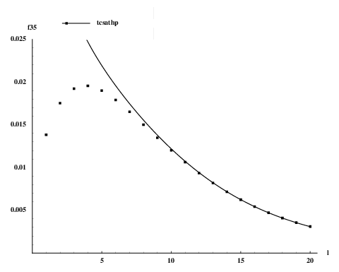
Figure (4.1) shows the comparison of eqn. (4.6) to numerical data obtained from Lee-Yang TCSA: the matching is spectacular, especially in the so-called scaling region (the volume range where residual finite size corrections are of the order of truncation errors, cf. [16]) where the relative deviation is less than 10−410^{-4}. Here and in all following plots we use the dimensionless volume parameter l=m​Ll=mL, and the matrix elements are also measured in units of mm (cf. [16] for details). Diagonal one-particle matrix elements for the Ising model are shown in figure 4.2, where we similarly use natural units given by the mass m=m1m=m_{1} of the lightest particle A1A_{1}, just as in all subsequent plots related to the Ising model.
Refer to caption
Figure 4.1: Diagonal 11-particle matrix elements in the scaling Lee-Yang model. The discrete points correspond to the TCSA data, while the continuous line corresponds to the prediction from exact form factors.
Refer to caption
(a) A1A_{1}–A1A_{1}
Refer to caption
(b) A2A_{2}–A2A_{2}
Figure 4.2: Diagonal 1-particle matrix elements in the Ising model. The discrete points correspond to the TCSA data, while the continuous line corresponds to the prediction from exact form factors.

One can use a similar argument to evaluate diagonal two-particle matrix elements in finite volume. Let us assume that the theory considered has diagonal scattering as in section 2.1. The two-particle Bethe-Yang equations remain valid even in a non-integrable theory as long as the total energy of the two-particle state remains under the inelastic threshold [38], and therefore the energy levels can be calculated from

mi1Lsinhθ~1+δ(θ~1−θ~2)\displaystyle m_{i_{1}}L\sinh\tilde{\theta}_{1}+\delta(\tilde{\theta}_{1}-\tilde{\theta}_{2}) =\displaystyle= 2​π​I1\displaystyle 2\pi I_{1}
mi2Lsinhθ~2+δ(θ~2−θ~1)\displaystyle m_{i_{2}}L\sinh\tilde{\theta}_{2}+\delta(\tilde{\theta}_{2}-\tilde{\theta}_{1}) =\displaystyle= 2​π​I2\displaystyle 2\pi I_{2}

and (up to residual finite size corrections)

E2(L)=E2​p​t(L)−E0(L)=mi1coshθ~1+mi2coshθ~2E_{2}(L)=E_{2pt}(L)-E_{0}(L)=m_{i_{1}}\cosh\tilde{\theta}_{1}+m_{i_{2}}\cosh\tilde{\theta}_{2}

where i1i_{1} and i2i_{2} label the particle species. After a somewhat tedious, but elementary calculation the variation of this energy difference with respect to λ\lambda can be determined, using (4.3) and (4.4):

Δ​E2​(L)\displaystyle\Delta E_{2}(L) =\displaystyle= λLρi1​i2​(θ~1,θ~2)(F4Ψ(θ~2+iπ,θ~1+iπ,θ~1,θ~2)i2​i1​i1​i2+mi1Lcoshθ~1F2Ψ(iπ,0)i2​i2\displaystyle\lambda\frac{L}{\rho_{i_{1}i_{2}}\left(\tilde{\theta}_{1},\tilde{\theta}_{2}\right)}\Big(F_{4}^{\Psi}\left(\tilde{\theta}_{2}+i\pi,\tilde{\theta}_{1}+i\pi,\tilde{\theta}_{1},\tilde{\theta}_{2}\right)_{i_{2}i_{1}i_{1}i_{2}}+m_{i_{1}}L\cosh\tilde{\theta}_{1}F_{2}^{\Psi}(i\pi,0)_{i_{2}i_{2}}
+mi2Lcoshθ~2FΨ(iπ,0)i1​i1)\displaystyle+m_{i_{2}}L\cosh\tilde{\theta}_{2}F^{\Psi}(i\pi,0)_{i_{1}i_{1}}\Big)

where all quantities (such as Bethe-Yang rapidities θ~i\tilde{\theta}_{i}, masses mim_{i} and the two-particle state density ρ2\rho_{2}) are in terms of the λ=0\lambda=0 theory. This result expresses the fact that there are two sources for the variation of two-particle energy levels: one is the mass shift of the individual particles, and the second is due to the variation in the interaction. On the other hand, in analogy with (4.5) we have

ΔE2(L)=λL(⟨{I1,I2}|Ψ|{I1,I2}⟩i1​i2,Li1​i2−⟨0|Ψ|0⟩L)\Delta E_{2}(L)=\lambda L\left({}_{i_{1}i_{2}}\langle\{I_{1},I_{2}\}|\Psi|\{I_{1},I_{2}\}\rangle_{i_{1}i_{2},L}-\langle 0|\Psi|0\rangle_{L}\right)

and so we obtain the following relation:

⟨{I1,I2}|Ψ|{I1,I2}⟩i1​i2,Li1​i2\displaystyle{}_{i_{1}i_{2}}\langle\{I_{1},I_{2}\}|\Psi|\{I_{1},I_{2}\}\rangle_{i_{1}i_{2},L} =\displaystyle= 1ρi1​i2​(θ~1,θ~2)​(F4Ψ​(θ~2+i​π,θ~1+i​π,θ~1,θ~2)i2​i1​i1​i2CLOSE\displaystyle\frac{1}{\rho_{i_{1}i_{2}}\left(\tilde{\theta}_{1},\tilde{\theta}_{2}\right)}\Big(F_{4}^{\Psi}\left(\tilde{\theta}_{2}+i\pi,\tilde{\theta}_{1}+i\pi,\tilde{\theta}_{1},\tilde{\theta}_{2}\right)_{i_{2}i_{1}i_{1}i_{2}} (4.7)
+mi1Lcoshθ~1F2Ψ(iπ,0)i2​i2\displaystyle+m_{i_{1}}L\cosh\tilde{\theta}_{1}F_{2}^{\Psi}(i\pi,0)_{i_{2}i_{2}}
+mi2Lcoshθ~2F2Ψ(iπ,0)i1​i1+⟨0|Ψ|0⟩)+…\displaystyle+m_{i_{2}}L\cosh\tilde{\theta}_{2}F_{2}^{\Psi}(i\pi,0)_{i_{1}i_{1}}+\langle 0|\Psi|0\rangle\Big)+\dots

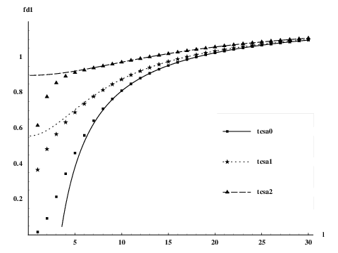
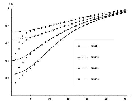
where the ellipsis again indicate residual finite size effects. The above argument is a generalization of the derivation of the mini-Hamiltonian coefficient CC in Appendix C of [15]. This formula is tested against numerical data in the Lee-Yang model in figure 4.3, and the agreement is as precise as it was for the one-particle case. Similar results can be found in the Ising case; they are shown in figure 4.4.
Refer to caption
Figure 4.3: Diagonal 22-particle matrix elements in the scaling Lee-Yang model. The discrete points correspond to the TCSA data, while the continuous line corresponds to the prediction from exact form factors.
Refer to caption
Figure 4.4: Diagonal 2-particle matrix elements in the Ising model. The discrete points correspond to the TCSA data, while the continuous line corresponds to the prediction from exact form factors.

4.2 Generalization to higher number of particles

Let us now introduce some more convenient notations. Given a state

|{I1​…​In}⟩i1​…​in|\{I_{1}\dots I_{n}\}\rangle_{i_{1}\dots i_{n}}

we denote

ρ​({k1,…,kr})L=ρik1​…​ikr​(θ~k1,…,θ~kr)\rho(\{k_{1},\dots,k_{r}\})_{L}=\rho_{i_{k_{1}}\dots i_{k_{r}}}(\tilde{\theta}_{k_{1}},\dots,\tilde{\theta}_{k_{r}}) (4.8)

where θ~l\tilde{\theta}_{l}, l=1,…,nl=1,\dots,n are the solutions of the nn-particle Bethe-Yang equations (2.9) at volume LL with quantum numbers I1,…,InI_{1},\dots,I_{n} and ρ⁡({k1,…,kr},L)\rho(\{k_{1},\dots,k_{r}\},L) is the rr-particle Bethe-Yang Jacobi determinant (2.10) involving only the rr-element subset 1≤k1<⋯<kr≤n1\leq k_{1}<\dots<k_{r}\leq n of the nn particles, evaluated with rapidities θ~k1,…,θ~kr\tilde{\theta}_{k_{1}},\dots,\tilde{\theta}_{k_{r}}. Let us further denote

ℱ​({k1,…,kr})L=F2​rs​(θ~k1,…,θ~kr)ik1​…​ikr\mathcal{F}(\{k_{1},\dots,k_{r}\})_{L}=F_{2r}^{s}(\tilde{\theta}_{k_{1}},\dots,\tilde{\theta}_{k_{r}})_{i_{k_{1}}\dots i_{k_{r}}}

where

F2​ns​(θ1,…,θn)i1​…​in=limϵ→0F2​nΨ​(θn+i​π+ϵ,…,θ1+i​π+ϵ,θ1,…,θn)i1​…​in​in​…​i1F_{2n}^{s}(\theta_{1},\dots,\theta_{n})_{i_{1}\dots i_{n}}=\lim_{\epsilon\rightarrow 0}F_{2n}^{\Psi}(\theta_{n}+i\pi+\epsilon,\dots,\theta_{1}+i\pi+\epsilon,\theta_{1},\dots,\theta_{n})_{i_{1}\dots i_{n}i_{n}\dots i_{1}} (4.9)

is the so-called symmetric evaluation of diagonal nn-particle matrix elements, which we analyze more closely in the next subsection. Note that the exclusion property mentioned at the end of subsection 2.1 carries over to the symmetric evaluation too: (4.9) vanishes whenever the rapidities of two particles of the same species coincide.

Based on the above results, we conjecture that the general rule for a diagonal matrix element takes the form of a sum over all bipartite divisions of the set of the nn particles involved (including the trivial ones when AA is the empty set or the complete set {1,…,n}\{1,\dots,n\}):

⟨{I1…In}|Ψ|{I1…In}⟩i1​…​in,Li1​…​in\,{}_{i_{1}\dots i_{n}}\langle\{I_{1}\dots I_{n}\}|\Psi|\{I_{1}\dots I_{n}\}\rangle_{i_{1}\dots i_{n},L} =\displaystyle= 1ρ​({1,…,n})L×\displaystyle\frac{1}{\rho(\{1,\dots,n\})_{L}}\times (4.10)
∑A⊂{1,2,…​n}ℱ​(A)L​ρ​({1,…,n}∖A)L+O⁡(e−μ​L)\displaystyle\sum_{A\subset\{1,2,\dots n\}}\mathcal{F}(A)_{L}\rho(\{1,\dots,n\}\setminus A)_{L}+O(\mathrm{e}^{-\mu L})

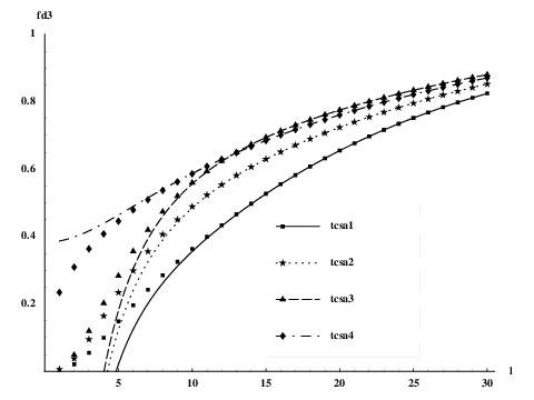
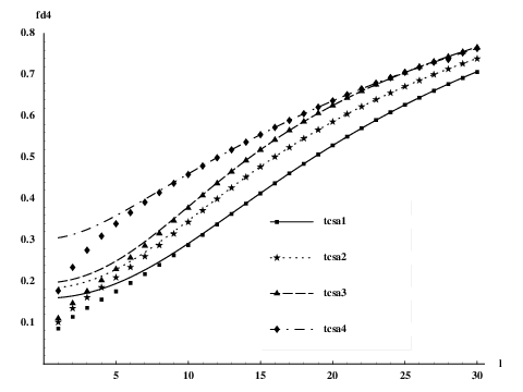
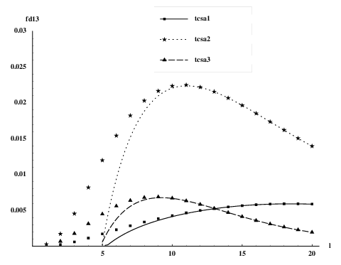
This rule can be tested against matrix elements with n=3n=3 and n=4n=4 in the Lee-Yang model, which are displayed in figures 4.5 and 4.6, respectively. The agreement is excellent as before, with the relative deviation in the scaling region being of the order of 10−410^{-4}.

Refer to caption
Figure 4.5: Diagonal 33-particle matrix elements in the scaling Lee-Yang model. The discrete points correspond to the TCSA data, while the continuous line corresponds to the prediction from exact form factors.
Refer to caption
Figure 4.6: Diagonal 44-particle matrix elements in the scaling Lee-Yang model. The discrete points correspond to the TCSA data, while the continuous line corresponds to the prediction from exact form factors.

5 Diagonal matrix elements in terms of connected form factors

In this section we discuss diagonal matrix elements in terms of connected form factors, and prove that a conjecture made by Saleur in [21] exactly coincides with our eqn. (4.10). To simplify notations we omit the particle species labels; they can be restored easily if needed.

5.1 Relation between connected and symmetric matrix elements

The purpose of this discussion is to give a treatment of the ambiguity inherent in diagonal matrix elements. Due to the existence of kinematical poles (2.6) the expression

F2​n​(θ1+i​π,θ2+i​π,…,θn+i​π,θn,…,θ2,θ1)F_{2n}(\theta_{1}+i\pi,\theta_{2}+i\pi,...,\theta_{n}+i\pi,\theta_{n},...,\theta_{2},\theta_{1})

which is relevant for diagonal multi-particle matrix elements, is not well-defined. Let us consider the regularized version

F2​n​(θ1+i​π+ϵ1,θ2+i​π+ϵ2,…,θn+i​π+ϵn,θn,…,θ2,θ1)F_{2n}(\theta_{1}+i\pi+\epsilon_{1},\theta_{2}+i\pi+\epsilon_{2},...,\theta_{n}+i\pi+\epsilon_{n},\theta_{n},...,\theta_{2},\theta_{1})

It was first observed in [36] that the singular parts of this expression drop when taking the limits ϵi→0\epsilon_{i}\rightarrow 0 simultaneously; however, the end result depends on the direction of the limit, i.e. on the ratio of the ϵi\epsilon_{i} parameters. The terms that are relevant in the limit can be written in the following general form:

F2​n​(θ1+i​π+ϵ1,θ2+i​π+ϵ2,…,θn+i​π+ϵn,θn,…,θ2,θ1)=\displaystyle F_{2n}(\theta_{1}+i\pi+\epsilon_{1},\theta_{2}+i\pi+\epsilon_{2},...,\theta_{n}+i\pi+\epsilon_{n},\theta_{n},...,\theta_{2},\theta_{1})= (5.1)
∏i=1n1ϵi⋅∑i1=1n∑i2=1n…​∑in=1nai1​i2​…​in​(θ1,…,θn)​ϵi1​ϵi2​…​ϵin+…\displaystyle\prod_{i=1}^{n}\frac{1}{\epsilon_{i}}\cdot\sum_{i_{1}=1}^{n}\sum_{i_{2}=1}^{n}...\sum_{i_{n}=1}^{n}a_{i_{1}i_{2}...i_{n}}(\theta_{1},\dots,\theta_{n})\epsilon_{i_{1}}\epsilon_{i_{2}}...\epsilon_{i_{n}}+\dots

where ai1​i2​…​ina_{i_{1}i_{2}...i_{n}} is a completely symmetric tensor of rank nn and the ellipsis denote terms that vanish when taking ϵi→0\epsilon_{i}\rightarrow 0 simultaneously.

In our previous considerations we used the symmetric limit, which is defined by taking all ϵi\epsilon_{i} equal:

F2​ns​(θ1,θ2,…,θn)=limϵ→0F2​n​(θ1+i​π+ϵ,θ2+i​π+ϵ,…,θn+i​π+ϵ,θn,…,θ2,θ1)F_{2n}^{s}(\theta_{1},\theta_{2},...,\theta_{n})=\lim_{\epsilon\to 0}F_{2n}(\theta_{1}+i\pi+\epsilon,\theta_{2}+i\pi+\epsilon,...,\theta_{n}+i\pi+\epsilon,\theta_{n},...,\theta_{2},\theta_{1})

It is symmetric in all the variables θ1,…,θn\theta_{1},\dots,\theta_{n}. There is another evaluation with this symmetry property, namely the so-called connected form factor, which is defined as the ϵi\epsilon_{i} independent part of eqn. (5.1), i.e. the part which does not diverge whenever any of the ϵi\epsilon_{i} is taken to zero:

F2​nc​(θ1,θ2,…,θn)=n!​a12​…​nF_{2n}^{c}(\theta_{1},\theta_{2},...,\theta_{n})=n!\,a_{12...n} (5.2)

where the appearance of the factor n!n! is simply due to the permutations of the ϵi\epsilon_{i}.

5.1.1 The relation for n≤3n\leq 3

We now spell out the relation between the symmetric and connected evaluations for n=1n=1, 22 and 33.

The n=1n=1 case is simple, since the two-particle form factor F2​(θ1,θ2)F_{2}(\theta_{1},\theta_{2}) has no singularities at θ1=θ2+i​π\theta_{1}=\theta_{2}+i\pi and therefore

F2s​(θ)=F2c​(θ)=F2​(i​π,0)F_{2}^{s}(\theta)=F_{2}^{c}(\theta)=F_{2}(i\pi,0) (5.3)

It is independent of the rapidities and will be denoted F2cF_{2}^{c} in the sequel.

For n=2n=2 we need to consider

F4​(θ1+i​π+ϵ1,θ2+i​π+ϵ2,θ2,θ1)≈a11​ϵ12+2​a12​ϵ1​ϵ2+a22​ϵ22ϵ1​ϵ2F_{4}(\theta_{1}+i\pi+\epsilon_{1},\theta_{2}+i\pi+\epsilon_{2},\theta_{2},\theta_{1})\approx\frac{a_{11}\epsilon_{1}^{2}+2a_{12}\epsilon_{1}\epsilon_{2}+a_{22}\epsilon_{2}^{2}}{\epsilon_{1}\epsilon_{2}} (5.4)

which gives

F4s​(θ1,θ2)\displaystyle F_{4}^{s}(\theta_{1},\theta_{2}) =\displaystyle= a11+2​a12+a22\displaystyle a_{11}+2a_{12}+a_{22}
F4c​(θ1,θ2)\displaystyle F_{4}^{c}(\theta_{1},\theta_{2}) =\displaystyle= 2​a12\displaystyle 2a_{12}

The terms a11a_{11} and a22a_{22} can be expressed using the two-particle form factor. Taking an infinitesimal, but fixed ϵ2≠0\epsilon_{2}\neq 0

Resϵ1=0F4​(θ1+i​π+ϵ1,θ2+i​π+ϵ2,θ2,θ1)=a22​ϵ2\mathop{\mathrm{Res}}_{\epsilon_{1}=0}F_{4}(\theta_{1}+i\pi+\epsilon_{1},\theta_{2}+i\pi+\epsilon_{2},\theta_{2},\theta_{1})=a_{22}\epsilon_{2}

whereas according to (2.7)

Resϵ1=0F4​(θ1+i​π+ϵ1,θ2+i​π+ϵ2,θ2,θ1)=i⁡(1−S⁡(θ1−θ2)​S​(θ1−θ2−i​π−ϵ2))​F2​(θ2+i​π+ϵ2,θ2)\mathop{\mathrm{Res}}_{\epsilon_{1}=0}F_{4}(\theta_{1}+i\pi+\epsilon_{1},\theta_{2}+i\pi+\epsilon_{2},\theta_{2},\theta_{1})=i\left(1-S(\theta_{1}-\theta_{2})S(\theta_{1}-\theta_{2}-i\pi-\epsilon_{2})\right)F_{2}(\theta_{2}+i\pi+\epsilon_{2},\theta_{2})

To first order in ϵ2\epsilon_{2}

S⁡(θ1−θ2−i​π−ϵ2)=S⁡(θ2−θ1+ϵ2)=S⁡(θ2−θ1)​(1+i​φ​(θ2−θ1)​ϵ2+…)S(\theta_{1}-\theta_{2}-i\pi-\epsilon_{2})=S(\theta_{2}-\theta_{1}+\epsilon_{2})=S(\theta_{2}-\theta_{1})(1+i\varphi(\theta_{2}-\theta_{1})\epsilon_{2}+\dots)

where

φ⁡(θ)=−i​dd​θ​log⁡S⁡(θ)\varphi(\theta)=-i\frac{d}{d\theta}\log S(\theta)

is the derivative of the two-particle phase shift defined before. Therefore we obtain

a22=φ⁡(θ2−θ1)​F2ca_{22}=\varphi(\theta_{2}-\theta_{1})F_{2}^{c}

and similarly

a11=φ⁡(θ1−θ2)​F2ca_{11}=\varphi(\theta_{1}-\theta_{2})F_{2}^{c}

and so

F4s​(θ1,θ2)=F4c​(θ1,θ2)+2​φ​(θ1−θ2)​F2​(i​π,0)F_{4}^{s}(\theta_{1},\theta_{2})=F_{4}^{c}(\theta_{1},\theta_{2})+2\varphi(\theta_{1}-\theta_{2})F_{2}(i\pi,0) (5.5)

In the case of the trace of the energy-momentum tensor Θ\Theta the following expressions are known [24]

F2Θ\displaystyle F_{2}^{\Theta} =\displaystyle= 2​π​m2\displaystyle 2\pi m^{2}
F4Θ,s\displaystyle F_{4}^{\Theta,s} =\displaystyle= 8​π​m2​φ​(θ1−θ2)​cosh2⁡(θ1−θ22)\displaystyle 8\pi m^{2}\varphi(\theta_{1}-\theta_{2})\cosh^{2}\left(\frac{\theta_{1}-\theta_{2}}{2}\right)
F4Θ,c\displaystyle F_{4}^{\Theta,c} =\displaystyle= 4​π​m2​φ​(θ1−θ2)​cosh⁡(θ1−θ2)\displaystyle 4\pi m^{2}\varphi(\theta_{1}-\theta_{2})\cosh(\theta_{1}-\theta_{2})

and they are in agreement with (5.5).

For n=3n=3, a procedure similar to the above gives the following relation:

F6s​(θ1,θ2,θ3)\displaystyle F_{6}^{s}(\theta_{1},\theta_{2},\theta_{3}) =\displaystyle= F6c​(θ1,θ2,θ3)+[F4c​(θ1,θ2)​(φ⁡(θ1−θ3)+φ⁡(θ2−θ3))+permutations]\displaystyle F_{6}^{c}(\theta_{1},\theta_{2},\theta_{3})+\left[F_{4}^{c}(\theta_{1},\theta_{2})(\varphi(\theta_{1}-\theta_{3})+\varphi(\theta_{2}-\theta_{3}))+\mathrm{permutations}\right] (5.6)
+3​F2c​[φ⁡(θ1−θ2)​φ​(θ1−θ3)+permutations]\displaystyle+3F_{2}^{c}\left[\varphi(\theta_{1}-\theta_{2})\varphi(\theta_{1}-\theta_{3})+\mathrm{permutations}\right]

where we omitted terms that only differ by permutation of the particles.

5.1.2 Relation between the connected and symmetric evaluation in the general case

Our goal is to compute the general expression

F2​n(θ1,…,θn|ϵ1,…,ϵn)=F2​n(θ1+iπ+ϵ1,θ2+iπ+ϵ2,…,θn+iπ+ϵn,θn,…,θ2,θ1)F_{2n}(\theta_{1},\dots,\theta_{n}|\epsilon_{1},\dots,\epsilon_{n})=F_{2n}(\theta_{1}+i\pi+\epsilon_{1},\theta_{2}+i\pi+\epsilon_{2},...,\theta_{n}+i\pi+\epsilon_{n},\theta_{n},...,\theta_{2},\theta_{1}) (5.7)

Let us take nn vertices labeled by the numbers 1,2,…,n1,2,\dots,n and let GG be the set of the directed graphs GiG_{i} with the following properties:

  • •

    GiG_{i} is tree-like.

  • •

    For each vertex there is at most one outgoing edge.

For an edge going from ii to jj we use the notation Ei​jE_{ij}.

Theorem 1

(5.7) can be evaluated as a sum over all graphs in GG, where the contribution of a graph GiG_{i} is given by the following two rules:

  • •

    Let Ai={a1,a2,…,am}A_{i}=\{a_{1},a_{2},\dots,a_{m}\} be the set of vertices from which there are no outgoing edges in GiG_{i}. The form factor associated to GiG_{i} is

    F2​mc​(θa1,θa2,…,θam)F_{2m}^{c}(\theta_{a_{1}},\theta_{a_{2}},\dots,\theta_{a_{m}}) (5.8)
  • •

    For each edge Ej​kE_{jk} the form factor above has to be multiplied by

    ϵjϵk​φ​(θj−θk)\frac{\epsilon_{j}}{\epsilon_{k}}\varphi(\theta_{j}-\theta_{k})

Note that since cannot contain cycles, the product of the ϵi/ϵj\epsilon_{i}/\epsilon_{j} factors will never be trivial (except for the empty graph with no edges).

Proof

The proof goes by induction in nn. For n=1n=1 we have

F2s​(θ1)=F2c​(θ1)=F2​(i​π,0)F_{2}^{s}(\theta_{1})=F_{2}^{c}(\theta_{1})=F_{2}(i\pi,0)

This is in accordance with the theorem, because for n=1n=1 there is only the trivial graph which contains no edges and a single node.

Now assume that the theorem is true for n−1n-1 and let us take the case of nn particles. Consider the residue of the matrix element (5.7) at ϵn=0\epsilon_{n}=0 while keeping all the ϵi\epsilon_{i} finite

R=Resϵn=0F2​n(θ1..θn|ϵ1..ϵn)R=\mathop{\mathrm{Res}}_{\epsilon_{n}=0}F_{2n}(\theta_{1}..\theta_{n}|\epsilon_{1}..\epsilon_{n})

According to the theorem the graphs contributing to this residue are exactly those for which the vertex nn has an outgoing edge and no incoming edges. Let RjR_{j} be sum of the diagrams where the outgoing edge is En​jE_{nj} for some j=1,…,n−1j=1,\dots,n-1, and so

R=∑j=1n−1RjR=\sum_{j=1}^{n-1}R_{j}

The form factors appearing in RjR_{j} do not depend on θn\theta_{n}. Therefore we get exactly the diagrams that are needed to evaluate F2​(n−1)(θ1..θn−1|ϵ1..ϵn−1)F_{2(n-1)}(\theta_{1}..\theta_{n-1}|\epsilon_{1}..\epsilon_{n-1}), apart from the proportionality factor associated to the link En​jE_{nj} and so

Rj=ϵjϵnφ(θj−θn)F2​(n−1)(θ1..θn−1|ϵ1..ϵn−1)R_{j}=\frac{\epsilon_{j}}{\epsilon_{n}}\varphi(\theta_{j}-\theta_{n})F_{2(n-1)}(\theta_{1}..\theta_{n-1}|\epsilon_{1}..\epsilon_{n-1})

and summing over jj gives

R=(ϵ1φ(θ1−θn)+ϵ2φ(θ2−θn)+⋯+ϵn−1φ(θn−1−θn))F2​(n−1)(θ1..θn−1|ϵ1..ϵn−1)R=(\epsilon_{1}\varphi(\theta_{1}-\theta_{n})+\epsilon_{2}\varphi(\theta_{2}-\theta_{n})+\dots+\epsilon_{n-1}\varphi(\theta_{n-1}-\theta_{n}))F_{2(n-1)}(\theta_{1}..\theta_{n-1}|\epsilon_{1}..\epsilon_{n-1}) (5.9)

In order to prove the theorem, we only need to show that the residue indeed takes this form. On the other hand, the kinematical residue axiom (2.6) gives

R=i(1−∏j=1n−1S(θn−θj)S(θn−θj−iπ−ϵj))F2​(n−1)(θ1..θn−1|ϵ1..ϵn−1)R=i\left(1-\prod_{j=1}^{n-1}S(\theta_{n}-\theta_{j})S(\theta_{n}-\theta_{j}-i\pi-\epsilon_{j})\right)F_{2(n-1)}(\theta_{1}..\theta_{n-1}|\epsilon_{1}..\epsilon_{n-1})

which is exactly the same as eqn. (5.9) when expanded to first order in ϵj\epsilon_{j}.

We thus checked that the theorem gives the correct result for the terms that include a 1/ϵn1/\epsilon_{n} singularity. Using symmetry in the rapidity variables this is true for all the terms that include at least one 1/ϵi1/\epsilon_{i} for an arbitrary ii. There is only one diagram that cannot be generated by the inductive procedure, namely the empty graph. However, there are no singularities (1/ϵi1/\epsilon_{i} factors) associated to it, and it gives F2​nc​(θ1,…,θn)F_{2n}^{c}(\theta_{1},\dots,\theta_{n}) by definition. Qed.

Refer to caption
Figure 5.1: The graphs relevant for n=2n=2

We now illustrate how the theorem works. For n=2n=2, there are only three graphs, depicted in figure 5.1. Applying the rules yields

F4(θ1,θ2|ϵ1,ϵ2)=F4c(θ1,θ2)+φ(θ1−θ2)(ϵ1ϵ2+ϵ2ϵ1)F2cF_{4}(\theta_{1},\theta_{2}|\epsilon_{1},\epsilon_{2})=F_{4}^{c}(\theta_{1},\theta_{2})+\varphi(\theta_{1}-\theta_{2})\left(\frac{\epsilon_{1}}{\epsilon_{2}}+\frac{\epsilon_{2}}{\epsilon_{1}}\right)F_{2}^{c}

which gives back (5.5) upon putting ϵ1=ϵ2\epsilon_{1}=\epsilon_{2}. For n=3n=3 there are 44 different kinds of graphs, the representatives of which are shown in figure 5.2; all other graphs can be obtained by permuting the node labels 1,2,31,2,3. The contributions of these graphs are

Refer to caption
Figure 5.2: The graphs relevant for n=3n=3
(a)\displaystyle(a) :\displaystyle: F6c​(θ1,θ2,θ3)\displaystyle F_{6}^{c}(\theta_{1},\theta_{2},\theta_{3})
(b)\displaystyle(b) :\displaystyle: ϵ2ϵ1​φ​(θ1−θ2)​F4c​(θ2,θ3)\displaystyle\frac{\epsilon_{2}}{\epsilon_{1}}\varphi(\theta_{1}-\theta_{2})F_{4}^{c}(\theta_{2},\theta_{3})
(c)\displaystyle(c) :\displaystyle: ϵ2ϵ1​ϵ3ϵ2​φ​(θ1−θ2)​φ​(θ2−θ3)​F2c=ϵ3ϵ1​φ​(θ1−θ2)​φ​(θ2−θ3)​F2c\displaystyle\frac{\epsilon_{2}}{\epsilon_{1}}\frac{\epsilon_{3}}{\epsilon_{2}}\varphi(\theta_{1}-\theta_{2})\varphi(\theta_{2}-\theta_{3})F_{2}^{c}=\frac{\epsilon_{3}}{\epsilon_{1}}\varphi(\theta_{1}-\theta_{2})\varphi(\theta_{2}-\theta_{3})F_{2}^{c}
(d)\displaystyle(d) :\displaystyle: ϵ2ϵ1​ϵ2ϵ3​φ​(θ1−θ2)​φ​(θ3−θ2)​F2c\displaystyle\frac{\epsilon_{2}}{\epsilon_{1}}\frac{\epsilon_{2}}{\epsilon_{3}}\varphi(\theta_{1}-\theta_{2})\varphi(\theta_{3}-\theta_{2})F_{2}^{c}

Adding up all the contributions and putting ϵ1=ϵ2=ϵ3\epsilon_{1}=\epsilon_{2}=\epsilon_{3} we recover eqn. (5.6).

5.2 Consistency with Saleur’s proposal

Saleur proposed an expression for diagonal matrix elements in terms of connected form factors in [21], which is partially based on earlier work by Balog [39] and also on the determinant formula for normalization of states in the framework of algebraic Bethe Ansatz, derived by Gaudin, and also by Korepin (see [40] and references therein). To describe it, we must extend the normalization of finite volume states defined in [16] to the case when the particle rapidities form a proper subset of some multi-particle Bethe-Yang solution.

According to [16], the normalization of a finite volume state is given by

|{I1,…,In}⟩L=1ρn​(θ~1,…,θ~n)|θ~1,…,θ~n⟩|\{I_{1},\dots,I_{n}\}\rangle_{L}=\frac{1}{\sqrt{\rho_{n}(\tilde{\theta}_{1},\dots,\tilde{\theta}_{n})}}|\tilde{\theta}_{1},\dots,\tilde{\theta}_{n}\rangle

in terms of the infinite volume state with rapidities θ~1,…,θ~n\tilde{\theta}_{1},\dots,\tilde{\theta}_{n}, which are the solutions of the Bethe-Yang equations (2.9) for the given quantum numbers I1,…,InI_{1},\dots,I_{n} at volume LL (we again omit the particle species labels, and also denote the nn-particle determinant by ρn\rho_{n}). Let us take a subset of particle indices A∈{1,…,n}A\in\{1,\dots,n\} and define the corresponding sub-determinant by

ρ~n​(θ~1,…,θ~n|A)=det𝒥A(n)\tilde{\rho}_{n}(\tilde{\theta}_{1},\dots,\tilde{\theta}_{n}|A)=\det\mathcal{J}_{A}^{(n)}

where 𝒥A(n)\mathcal{J}_{A}^{(n)} is the sub-matrix of the matrix 𝒥(n)\mathcal{J}^{(n)} defined in eqn. (2.10) which is given by choosing the elements whose indices belong to AA. The full matrix can be written explicitly as

𝒥(n)=(E1​L+φ12+⋯+φ1​n−φ12…−φ1​n−φ12E2​L+φ21+φ23+⋯+φ2​n…−φ2​n⋱−φ1​n−φ2​n…En​L+φ1​n+⋯+φn−1,n)\mathcal{J}^{(n)}=\begin{pmatrix}E_{1}L+\varphi_{12}+\dots+\varphi_{1n}&-\varphi_{12}&\dots&-\varphi_{1n}\\ -\varphi_{12}&E_{2}L+\varphi_{21}+\varphi_{23}+\dots+\varphi_{2n}&\dots&-\varphi_{2n}\\ \vdots&\vdots&\ddots&\vdots\\ -\varphi_{1n}&-\varphi_{2n}&\dots&E_{n}L+\varphi_{1n}+\dots+\varphi_{n-1,n}\end{pmatrix}

where the following abbreviations were used: Ei=micoshθiE_{i}=m_{i}\cosh\theta_{i}, φi​j=φj​i=φ⁡(θi−θj)\varphi_{ij}=\varphi_{ji}=\varphi(\theta_{i}-\theta_{j}). Note that ρ~n\tilde{\rho}_{n} depends on all the rapidities, not just those which correspond to elements of AA. It is obvious that

ρn​(θ~1,…,θ~n)≡ρ~n​(θ~1,…,θ~n|{1,…,n})\rho_{n}(\tilde{\theta}_{1},\dots,\tilde{\theta}_{n})\equiv\tilde{\rho}_{n}(\tilde{\theta}_{1},\dots,\tilde{\theta}_{n}|\{1,\dots,n\})

Saleur proposed the definition

⟨{θ~k}k∈A|{θ~k}k∈A⟩L=ρ~n​(θ~1,…,θ~n|A)\langle\{\tilde{\theta}_{k}\}_{k\in A}|\{\tilde{\theta}_{k}\}_{k\in A}\rangle_{L}=\tilde{\rho}_{n}(\tilde{\theta}_{1},\dots,\tilde{\theta}_{n}|A) (5.10)

where

|{θ~k}k∈A⟩L|\{\tilde{\theta}_{k}\}_{k\in A}\rangle_{L}

is a “partial state” which contains only the particles with index in AA, but with rapidities that solve the Bethe-Yang equations for the full nn-particle state. Note that this is not a proper state in the sense that it is not an eigenstate of the Hamiltonian since the particle rapidities do not solve the Bethe-Yang equations relevant for a state consisting of |A||A| particles (where |A||A| denotes the cardinal number – i.e. number of elements – of the set AA). The idea behind this proposal is that the density of these partial states in rapidity space depends on the presence of the other particles which are not included, and indeed it is easy to see that it is given by ρ~n​(θ~1,…,θ~n|A)\tilde{\rho}_{n}(\tilde{\theta}_{1},\dots,\tilde{\theta}_{n}|A).

In terms of the above definitions, Saleur’s conjecture for the diagonal matrix element is

⟨{I1…In}|Ψ|{I1…In}⟩i1​…​in,Li1​…​in\,{}_{i_{1}\dots i_{n}}\langle\{I_{1}\dots I_{n}\}|\Psi|\{I_{1}\dots I_{n}\}\rangle_{i_{1}\dots i_{n},L} =\displaystyle= 1ρn​(θ~1,…,θ~n)×\displaystyle\frac{1}{\rho_{n}(\tilde{\theta}_{1},\dots,\tilde{\theta}_{n})}\times (5.11)
∑A⊂{1,2,…​n}F2​|A|c​({θ~k}k∈A)​ρ~​(θ~1,…,θ~n|A)+O⁡(e−μ​L)\displaystyle\sum_{A\subset\{1,2,\dots n\}}F_{2|A|}^{c}(\{\tilde{\theta}_{k}\}_{k\in A})\tilde{\rho}(\tilde{\theta}_{1},\dots,\tilde{\theta}_{n}|A)+O(\mathrm{e}^{-\mu L})

which is just the standard representation of the full matrix element as the sum of all the connected contributions provided we accept eqn. (5.10). The full amplitude is obtained by summing over all possible bipartite divisions of the particles, where the division is into particles that are connected to the local operator, giving the connected form factor FcF^{c} and into those that simply go directly from the initial to the final state which contribute the norm of the corresponding partial multi-particle state.

Using the results of subsection 5.1, it is easy to check explicitly (which we did up to n=3n=3) that our rule for the diagonal matrix elements as given in eqn. (4.10) is equivalent to eqn. (5.11). We now give a complete proof for the general case.

Theorem 2
∑A⊂NF2​|A|c​({θk}k∈A)​ρ~​(θ1,…,θn|A)=∑A⊂NF2​|A|s​({θk}k∈A)​ρ​({θk}k∈N∖A)\sum_{A\subset N}F_{2|A|}^{c}(\{\theta_{k}\}_{k\in A})\tilde{\rho}(\theta_{1},\dots,\theta_{n}|A)=\sum_{A\subset N}F_{2|A|}^{s}(\{\theta_{k}\}_{k\in A})\rho(\{\theta_{k}\}_{k\in N\setminus A}) (5.12)

where we denoted N={1,2,…,n}N=\{1,2,\dots,n\}.

Proof

The two sides of eqn. (5.12) differ in two ways:

  • •

    The form factors on the right hand side are evaluated according to the ,,symmetric” prescription, and in addition to the connected part also they contain extra terms, which are proportional to connected form factors with fewer particles.

  • •

    The densities ρ~\tilde{\rho} on the left hand side are not determinants of the form (2.10) written down in terms of the particles contained in N∖AN\setminus A: they contain additional terms due to the presence of the particles in AA as well.

Here we show that eqn. (5.12) is merely a reorganization of these terms.

For simplicity consider first the term on the left hand side which corresponds to A={m+1,m+2,…,n}A=\{m+1,m+2,\dots,n\}, i.e.

F2​mc​(θm+1,…,θn)​ρ~​(θ1,…,θn|A)F_{2m}^{c}(\theta_{m+1},\dots,\theta_{n})\tilde{\rho}(\theta_{1},\dots,\theta_{n}|A)

We expand ρ~\tilde{\rho} in terms of the physical multi-particle densities ρ\rho. In order to accomplish this, it is useful to rewrite the sub-matrix 𝒥N∖An\mathcal{J}_{N\setminus A}^{n}{} as

𝒥(n)|N∖A=𝒥m​(θ1,…,θm)+(∑i=m+1nφ1​i∑i=m+1nφ2​i⋱∑i=m+1nφm​i)\mathcal{J}^{(n)}|_{N\setminus A}=\mathcal{J}^{m}(\theta_{1},\dots,\theta_{m})+\begin{pmatrix}\sum\limits_{i=m+1}^{n}\varphi_{1i}\\ &&\sum\limits_{i=m+1}^{n}\varphi_{2i}\\ &&&&\ddots\\ &&&&&&\sum\limits_{i=m+1}^{n}\varphi_{mi}\end{pmatrix}

where 𝒥m\mathcal{J}^{m} is the mm-particle Jacobian matrix which does not contain any terms depending on the particles in AA. The determinant of 𝒥N∖An\mathcal{J}_{N\setminus A}^{n}{} can be written as a sum over the subsets of N∖AN\setminus A. For a general subset B⊂N∖AB\subset N\setminus A let us use the notation B={b1,b2,…,b|B|}B=\{b_{1},b_{2},\dots,b_{|B|}\}. We can then write

ρ~​(θ1,…,θn|A)=det​𝒥(n)|N∖A=∑B[ρ⁡(N∖(A∪B))​∏i=1|B|(∑ci=m+1nφbi,ci)]\tilde{\rho}(\theta_{1},\dots,\theta_{n}|A)=\text{det}\mathcal{J}^{(n)}|_{N\setminus A}=\sum_{B}\left[\rho(N\setminus(A\cup B))\prod_{i=1}^{|B|}\left(\sum_{c_{i}=m+1}^{n}\varphi_{b_{i},c_{i}}\right)\right] (5.13)

where ρ⁡(N∖(A∪B))\rho(N\setminus(A\cup B)) is the ρ\rho-density (2.10) written down with the particles in N∖(A∪B)N\setminus(A\cup B).

Applying a suitable permutation of variables we can generalize eqn. (5.13) to an arbitrary subset A⊂NA\subset N:

ρ~​(θ1,…,θn|A)=det​𝒥(n)|N∖A=∑Bρ⁡(N∖(A∪B))​∑C(∏i=1|B|φbi,ci)\tilde{\rho}(\theta_{1},\dots,\theta_{n}|A)=\text{det}\mathcal{J}^{(n)}|_{N\setminus A}=\sum_{B}\rho(N\setminus(A\cup B))\sum_{C}(\prod_{i=1}^{|B|}\varphi_{b_{i},c_{i}}) (5.14)

where the second summation goes over all the sets C={c1,c2,…,c|B|}C=\{c_{1},c_{2},\dots,c_{|B|}\} with |C|=|B||C|=|B| and ci∈Ac_{i}\in A. The left hand side of eqn. (5.12) can thus be written as

∑A⊂NF2​|A|c​({θk}k∈A)​ρ~​(θ1,…,θn|A)\displaystyle\sum_{A\subset N}F_{2|A|}^{c}(\{\theta_{k}\}_{k\in A})\tilde{\rho}(\theta_{1},\dots,\theta_{n}|A) =\displaystyle= ∑A,B⊂NA∩B=∅ρ⁡(N∖(A∪B))​∑CF(A,B,C)\displaystyle\sum_{\begin{array}[]{c}A,B\subset N\\ A\cap B=\emptyset\end{array}}\rho(N\setminus(A\cup B))\sum_{C}F_{(A,B,C)}
where F(A,B,C)=F2​|A|c​({θk}k∈A)​∏i=1|B|φbi,ci\displaystyle F_{(A,B,C)}=F_{2|A|}^{c}(\{\theta_{k}\}_{k\in A})\prod_{i=1}^{|B|}\varphi_{b_{i},c_{i}}

We now show that there is a one-to-one correspondence between all the terms in (5.2) and those on the right hand side of (5.12) if the symmetric evaluations F2​ksF_{2k}^{s} are expanded according to Theorem 1. To each triplet (A,B,C)(A,B,C) let us assign the graph G(A,B,C)G_{(A,B,C)} defined as follows:

  • •

    The vertices of the graph are the elements of the set A∪BA\cup B.

  • •

    There are exactly |B||B| edges in the graph, which start at bib_{i} and end at cic_{i} with i=1,…,|B|i=1,\dots,|B|.

The contribution of G(A,B,C)G_{(A,B,C)} to F2​(|A|+|B|)s​({θk}k∈A∪B)F_{2(|A|+|B|)}^{s}(\{\theta_{k}\}_{k\in A\cup B}) is nothing else than F(A,B,C)F_{(A,B,C)} which can be proved by applying the rules of Theorem 1. Note that all the possible diagrams with at most nn vertices are contained in the above list of the G(A,B,C)G_{(A,B,C)}, because a general graph GG satisfying the conditions in Theorem 1 can be characterized by writing down the set of vertices with and without outgoing edges (in this case BB and AA) and the endpoints of the edges (in this case CC).

It is easy to see that the factors ρ⁡(N∖(A∪B))\rho(N\setminus(A\cup B)) multiplying the F(A,B,C)F_{(A,B,C)} in (5.2) are also the correct ones: they are just the density factors multiplying F2​(|A|+|B|)s​({θk}k∈A∪B)F_{2(|A|+|B|)}^{s}(\{\theta_{k}\}_{k\in A\cup B}) on the right hand side of (5.12). Qed.

6 Zero-momentum particles

6.1 Scaling Lee-Yang model

In the scaling Lee-Yang model, with a single type of particle, there can only be a single particle of zero momentum in a multi-particle state due to the exclusion principle. For the momentum to be exactly zero in finite volume it is necessary that the all other particles should come with quantum numbers in pairs of opposite sign, which means that the state must have 2​n+12n+1 particles in a configuration

|{I1,…,In,0,−In,…,−I1}⟩L|\{I_{1},\dots,I_{n},0,-I_{n},\dots,-I_{1}\}\rangle_{L}

Therefore we consider matrix elements of the form

⟨{I1′,…,Ik′,0,−Ik′,…,−I1′}|Φ|{I1,…,Il,0,−Il,…,−I1}⟩L\langle\{I_{1}^{\prime},\dots,I_{k}^{\prime},0,-I_{k}^{\prime},\dots,-I_{1}^{\prime}\}|\Phi|\{I_{1},\dots,I_{l},0,-I_{l},\dots,-I_{1}\}\rangle_{L}

(with k=0k=0 or l=0l=0 corresponding to a state containing a single stationary particle). We also suppose that the two sets {I1,…,Ik}\{I_{1},\dots,I_{k}\} and {I1′,…,Il′}\{I_{1}^{\prime},\dots,I_{l}^{\prime}\} are not identical, otherwise we have the case of diagonal matrix elements treated in section 4.

We need to examine form factors of the form

F2​k+2​l+2​(i​π+θ1′,…,i​π+θk′,i​π−θk′,…,i​π−θ1′,i​π+θ,0,θ1,…,θl,−θl,…,−θ1)F_{2k+2l+2}(i\pi+\theta_{1}^{\prime},\dots,i\pi+\theta_{k}^{\prime},i\pi-\theta_{k}^{\prime},\dots,i\pi-\theta_{1}^{\prime},i\pi+\theta,0,\theta_{1},\dots,\theta_{l},-\theta_{l},\dots,-\theta_{1})

where the particular ordering of the rapidities was chosen to ensure that no additional SS matrix factors appear in the disconnected terms of the crossing relation (2.2). Using the singularity axiom (2.6), plus unitarity and crossing symmetry of the SS-matrix it is easy to see that the residue of the above function at θ=0\theta=0 vanishes, and so it has a finite limit as θ→0\theta\rightarrow 0. However, this limit depends on direction just as in the case of the diagonal matrix elements considered in section 4. Therefore we must specify the way it is taken, and just as previously we use a prescription that is maximally symmetric in all variables: we choose to shift all rapidities entering the left hand state with the same amount to define

ℱk,l(θ1′,…,θk′|θ1,…,θl)=\displaystyle\mathcal{F}_{k,l}(\theta_{1}^{\prime},\dots,\theta_{k}^{\prime}|\theta_{1},\dots,\theta_{l})=
limϵ→0F2​k+2​l+2​(i​π+θ1′+ϵ,…,i​π+θk′+ϵ,i​π−θk′+ϵ,…,i​π−θ1′+ϵCLOSE,\displaystyle\lim_{\epsilon\rightarrow 0}F_{2k+2l+2}(i\pi+\theta_{1}^{\prime}+\epsilon,\dots,i\pi+\theta_{k}^{\prime}+\epsilon,i\pi-\theta_{k}^{\prime}+\epsilon,\dots,i\pi-\theta_{1}^{\prime}+\epsilon,
OPENi​π+ϵ,0,θ1,…,θl,−θl,…,−θ1)\displaystyle i\pi+\epsilon,0,\theta_{1},\dots,\theta_{l},-\theta_{l},\dots,-\theta_{1}) (6.1)

Using the above definition, by analogy to (4.10) we conjecture that

f2​k+1,2​l+1\displaystyle f_{2k+1,2l+1} =\displaystyle= ⟨{I1′,…,Ik′,0,−Ik′,…,−I1′}|Φ|{I1,…,Il,0,−Il,…,−I1}⟩L\displaystyle\langle\{I_{1}^{\prime},\dots,I_{k}^{\prime},0,-I_{k}^{\prime},\dots,-I_{1}^{\prime}\}|\Phi|\{I_{1},\dots,I_{l},0,-I_{l},\dots,-I_{1}\}\rangle_{L} (6.2)
=\displaystyle= 1ρ2​k+1​(θ~1′,…,θ~k′,0,−θ~k′,…,−θ~1′)​ρ2​l+1​(θ~1,…,θ~l,0,−θ~l,…,−θ~1)×\displaystyle\frac{1}{\sqrt{\rho_{2k+1}(\tilde{\theta}_{1}^{\prime},\dots,\tilde{\theta}_{k}^{\prime},0,-\tilde{\theta}_{k}^{\prime},\dots,-\tilde{\theta}_{1}^{\prime})\rho_{2l+1}(\tilde{\theta}_{1},\dots,\tilde{\theta}_{l},0,-\tilde{\theta}_{l},\dots,-\tilde{\theta}_{1})}}\times
(ℱk,l(θ~1′,…,θ~k′|θ~1,…,θ~l)+mLF2​k+2​l(iπ+θ~1′,…,iπ+θ~k′,\displaystyle\Big(\mathcal{F}_{k,l}(\tilde{\theta}_{1}^{\prime},\dots,\tilde{\theta}_{k}^{\prime}|\tilde{\theta}_{1},\dots,\tilde{\theta}_{l})+mL\,F_{2k+2l}(i\pi+\tilde{\theta}_{1}^{\prime},\dots,i\pi+\tilde{\theta}_{k}^{\prime},
OPENOPENi​π−θ~k′,…,i​π−θ~1′,θ~1,…,θ~l,−θ~l,…,−θ~1))+O⁡(e−μ​L)\displaystyle i\pi-\tilde{\theta}_{k}^{\prime},\dots,i\pi-\tilde{\theta}_{1}^{\prime},\tilde{\theta}_{1},\dots,\tilde{\theta}_{l},-\tilde{\theta}_{l},\dots,-\tilde{\theta}_{1})\Big)+O(\mathrm{e}^{-\mu L})

where θ~\tilde{\theta} denote the solutions of the appropriate Bethe-Yang equations at volume LL, ρn\rho_{n} is a shorthand notation for the nn-particle Bethe-Yang density (2.10) and equality is understood up to phase factors. We recall from our previous work [16] that relative phases of multi-particle states are in general fixed differently in the form factor bootstrap and TCSA. Also note that reordering particles gives phase factors on the right hand side according to the exchange axiom (2.4). This issue is obviously absent in the case of diagonal matrix elements treated in sections 4 and 5, since any such phase factor cancels out between the state and its conjugate. Such phases do not affect correlation functions, or as a consequence, any physically relevant quantities since they can all be expressed in terms of correlators.

There is some argument that can be given in support of eqn. (6.2). Note that the zero-momentum particle occurs in both the left and right states, which actually makes it unclear how to define a density similar to ρ~\tilde{\rho} in (5.10). Such a density would take into account the interaction with the other particles. However, the nonzero rapidities entering of the two states are different and therefore there is no straightforward way to apply Saleur’s recipe (5.11) here. Using the maximally symmetric definition (6.1) the shift ϵ\epsilon can be equally put on the right hand side rapidities as well, and therefore we expect that the density factor multiplying the term F2​k+2​lF_{2k+2l} in (6.2) would be the one-particle state density in which none of the other rapidities appear, which is exactly m​LmL for a stationary particle. This is a natural guess from eqn. (4.10) which states that when diagonal matrix elements are expressed using the symmetric evaluation, only densities of the type ρ\rho appear.

Another argument can be formulated using the observation that eqn. (6.2) is only valid if ℱk,l\mathcal{F}_{k,l} is defined as in (6.1); all other possible ways to take the limit can be related in a simple way to this definition and so the rule (6.2) can be rewritten appropriately. Let us consider two other natural choices

ℱk,l+(θ1′,…,θk′|θ1,…,θl)=\displaystyle\mathcal{F}_{k,l}^{+}(\theta_{1}^{\prime},\dots,\theta_{k}^{\prime}|\theta_{1},\dots,\theta_{l})=
limϵ→0F2​k+2​l+2​(i​π+θ1′,…,i​π+θk′,i​π−θk′,…,i​π−θ1′,i​π,ϵ,θ1,…,θl,−θl,…,−θ1)\displaystyle\lim_{\epsilon\rightarrow 0}F_{2k+2l+2}(i\pi+\theta_{1}^{\prime},\dots,i\pi+\theta_{k}^{\prime},i\pi-\theta_{k}^{\prime},\dots,i\pi-\theta_{1}^{\prime},i\pi,\epsilon,\theta_{1},\dots,\theta_{l},-\theta_{l},\dots,-\theta_{1})
ℱk,l−(θ1′,…,θk′|θ1,…,θl)=\displaystyle\mathcal{F}_{k,l}^{-}(\theta_{1}^{\prime},\dots,\theta_{k}^{\prime}|\theta_{1},\dots,\theta_{l})=
limϵ→0F2​k+2​l+2​(i​π+θ1′,…,i​π+θk′,i​π−θk′,…,i​π−θ1′,i​π+ϵ,0,θ1,…,θl,−θl,…,−θ1)\displaystyle\lim_{\epsilon\rightarrow 0}F_{2k+2l+2}(i\pi+\theta_{1}^{\prime},\dots,i\pi+\theta_{k}^{\prime},i\pi-\theta_{k}^{\prime},\dots,i\pi-\theta_{1}^{\prime},i\pi+\epsilon,0,\theta_{1},\dots,\theta_{l},-\theta_{l},\dots,-\theta_{1})

in which the shift is put only on the zero-momentum particle on the right/left, respectively. Using the kinematical residue axiom (2.6), ℱ±\mathcal{F}^{\pm} can be related to ℱ\mathcal{F} via

ℱk,l(θ1′,…,θk′|θ1,…,θl)=ℱk,l+(θ1′,…,θk′|θ1,…,θl)\displaystyle\mathcal{F}_{k,l}(\theta_{1}^{\prime},\dots,\theta_{k}^{\prime}|\theta_{1},\dots,\theta_{l})=\mathcal{F}_{k,l}^{+}(\theta_{1}^{\prime},\dots,\theta_{k}^{\prime}|\theta_{1},\dots,\theta_{l})
+2∑i=1lφ(θi)F2​k+2​l(iπ+θ1′,…,iπ+θk′,iπ−θk′,…,iπ−θ1′,θ1,…,θl,−θl,…,−θ1)\displaystyle+2\sum_{i=1}^{l}\varphi(\theta_{i})F_{2k+2l}(i\pi+\theta_{1}^{\prime},\dots,i\pi+\theta_{k}^{\prime},i\pi-\theta_{k}^{\prime},\dots,i\pi-\theta_{1}^{\prime},\theta_{1},\dots,\theta_{l},-\theta_{l},\dots,-\theta_{1})
ℱk,l(θ1′,…,θk′|θ1,…,θl)=ℱk,l−(θ1′,…,θk′|θ1,…,θl)\displaystyle\mathcal{F}_{k,l}(\theta_{1}^{\prime},\dots,\theta_{k}^{\prime}|\theta_{1},\dots,\theta_{l})=\mathcal{F}_{k,l}^{-}(\theta_{1}^{\prime},\dots,\theta_{k}^{\prime}|\theta_{1},\dots,\theta_{l})
−2∑i=1kφ(θi′)F2​k+2​l(iπ+θ1′,…,iπ+θk′,iπ−θk′,…,iπ−θ1′,θ1,…,θl,−θl,…,−θ1)\displaystyle-2\sum_{i=1}^{k}\varphi(\theta_{i}^{\prime})F_{2k+2l}(i\pi+\theta_{1}^{\prime},\dots,i\pi+\theta_{k}^{\prime},i\pi-\theta_{k}^{\prime},\dots,i\pi-\theta_{1}^{\prime},\theta_{1},\dots,\theta_{l},-\theta_{l},\dots,-\theta_{1})

With the help of the above relations eqn. (6.2) can also be rewritten in terms of ℱ±\mathcal{F}^{\pm}. The way ℱ\mathcal{F} and therefore also eqn. (6.2) are expressed in terms of ℱ±\mathcal{F^{\pm}} shows a remarkable and natural symmetry under the exchange of the left and right state (and correspondingly ℱ+\mathcal{F}^{+} with ℱ−\mathcal{F}^{-}), which provides a further support to our conjecture.
Refer to caption
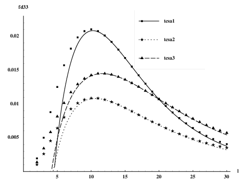
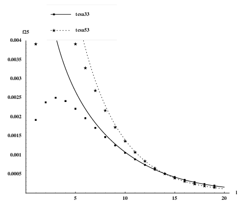
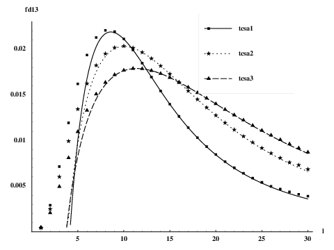
Figure 6.1: 11-particle–33-particle matrix elements in the scaling Lee-Yang model. The discrete points correspond to the TCSA data, while the continuous line corresponds to the prediction from exact form factors.
Refer to caption
Figure 6.2: 33-particle–33-particle matrix elements in the scaling Lee-Yang model. The discrete points correspond to the TCSA data, while the continuous line corresponds to the prediction from exact form factors.

The above two arguments cannot be considered as a proof; we do not have a proper derivation of relation (6.2) at the moment. On the other hand, as we now show it agrees very well with numerical data which would be impossible if there were some additional φ\varphi terms present; such terms, as shown in our previous work [16] would contribute corrections of order 1/l1/l in terms of the dimensionless volume parameter l=m​Ll=mL.

Data for the case of 11-33 and 33-33 matrix elements are shown in figures 6.1 and 6.2, respectively. In order to strengthen the support for eqn. (6.2) we must find 55-particle states. This is not easy because they are high up in the spectrum, and identification using the process of matching against Bethe-Yang predictions (as described in [16]) becomes ambiguous. We could identify the first 55-particle state by combining the Bethe-Yang matching with predictions for matrix elements with no disconnected pieces given by eqn. (2.11), as shown in figure 6.3. Some care must be taken in choosing the other state because many choices give matrix elements that are too small to be measured reliably in TCSA: since vector components and TCSA matrices are mostly of order 11 or slightly less, getting a result of order 10−410^{-4} or smaller involves a lot of cancellation between a large number of individual contributions, which inevitably leads to the result being dominated by truncation errors. Despite these difficulties, combining Bethe-Yang level matching with form factor evaluation we could identify the first five-particle level up to l=20l=20.

Refer to caption

Refer to caption

Figure 6.3: Identifying the 55-particle state using form factors. The discrete points correspond to the TCSA data, while the continuous line corresponds to the prediction from exact form factors.

The simplest matrix element involving a five-particle state and zero-momentum disconnected pieces is the 11-55 one, but the prediction of eqn. (6.2) turns out to be too small to be usefully compared to TCSA. However, it is possible to find 33-55 matrix elements that are sufficiently large, and the data shown in figure 6.4 confirm our conjecture with a relative precision of somewhat better than 10−310^{-3} in the scaling region.

Refer to caption
Figure 6.4: 33-particle–55-particle matrix elements in the scaling Lee-Yang model. The discrete points correspond to the TCSA data, while the continuous line corresponds to the prediction from exact form factors.

We close by noting that since the agreement is better than one part in 10310^{3} in the scaling region, which is typically found in the range of volume l∼10​…​20l\sim 10\dots 20, and also this precision holds for quite a large number of independent matrix elements, the presence of additional φ\varphi terms in eqn. (6.2) can be confidently excluded.

6.2 Ising model in magnetic field

In figure 6.5 we show how the prediction (6.2) describes a 11-33 matrix element in the Ising model; since all particles in this example are of species A1A_{1}, the formula carries over without essential modifications.

Refer to caption
Figure 6.5: A1−A1​A1​A1A_{1}-A_{1}A_{1}A_{1} matrix element in Ising model with a zero-momentum particle

However, due to the fact that the Ising model has more than one particle species, it is possible to have more than one stationary particles in the same state. Our TCSA data allow us to locate one such state, with a stationary A1A_{1} and A2A_{2} particle, and extending our previous considerations we have the prediction

f1,12=⟨{0}|Ψ|{0,0}⟩121=1m1​L​m2​L(limϵ→0F3(iπ+ϵ,0,0)112+m1LF1(0)2)f_{1,12}={}_{1}\langle\{0\}|\Psi|\{0,0\}\rangle_{12}=\frac{1}{m_{1}L\sqrt{m_{2}L}}\left(\lim_{\epsilon\rightarrow 0}F_{3}(i\pi+\epsilon,0,0)_{112}+m_{1}L\,F_{1}(0)_{2}\right)

where F1​(0)2F_{1}(0)_{2} is the one-particle form factor corresponding to A2A_{2}. This is compared to TCSA data in figure 6.6 and a convincing agreement is found.

Note that in both of figures 6.5 and 6.6 there is a point which obviously deviates from the prediction. This is a purely technical issue, and is due to the presence of a line crossing close to this particular value of the volume which makes the cutoff dependence more complicated and so slightly upsets the extrapolation in the cutoff. We also remark that we cannot check further matrix elements at the moment, because the appropriate form factor solutions have not yet been computed.

Refer to caption
Figure 6.6: A1−A1​A2A_{1}-A_{1}A_{2} matrix element in Ising model with zero-momentum particle

7 Finite temperature correlators

In this section we show how a systematical low-temperature expansion for correlation functions can be developed using the results presented so far. Finite temperature correlation functions have attracted quite a lot of interest recently. Leclair and Mussardo proposed an expansion for the one-point and two-point functions in terms of form factors dressed by appropriate occupation number factors containing the TBA pseudo-energy function [20], based on a quasi-particle description motivated by the thermodynamic Bethe Ansatz. As discussed in the introduction, their proposal for the two-point function was shown to be incorrect by Saleur [21]; on the other hand, he also gave a proof of the Leclair-Mussardo formula for one-point functions based on the conjecture formulated in eqn. (5.11), provided the operator considered is the density of some local conserved charge. Since we proved that our formula (4.10) for diagonal matrix elements is equivalent to Saleur’s conjecture, our results in section 4 can be considered as a very convincing numerical evidence for the correctness of his argument.

Another proposal for finite-temperature one-point functions was made by Delfino [23], who attempted to express them in terms of free-particle occupation numbers and the symmetric evaluation of diagonal matrix elements. It was shown by Mussardo that this proposal is not correct using a counter example where it disagreed with the Leclair-Mussardo expansion [24].

Furthermore, Castro-Alvaredo and Fring also argued [25] that two-point functions cannot be obtained by a simple dressing procedure analogous to the Leclair-Mussardo expansion for one-point functions. They argued that one needs a more drastic change in the form factor program.

All these issues are connected to the problem of finding a proper definition of the disconnected pieces. From the crossing relation (2.2), these are infinite for the form factors defined in infinite volume, and subtraction of such infinities must be made with care in order to obtain the correct finite pieces. Because of the above difficulties there is also a development in the direction of finite temperature form factors (for a review cf. [41]); with further development, this other line of thought can also give a very useful formulation of finite temperature correlation functions.

Here we use the idea that putting the system into a finite volume LL provides a regularization for the form factors, which can even be considered physical since in the real world there are no infinite systems11 1 There is actually a little subtlety here, since we impose periodic boundary conditions which are also nonphysical, but we make use of the old intuition that nothing can actually depend very much on the choice of the boundary condition if the system is very large and has a finite correlation length (i.e. a mass gap).. Our expressions for the finite volume form factors are valid up to exponential corrections in the volume, which makes it clear that performing the calculation in finite volume and then taking the limit L→∞L\rightarrow\infty we should recover the proper finite temperature correlation function. Here we present the computation for the case of the one-point function up to the first three nontrivial orders; the calculation gets complicated for higher orders, but the recipe is straightforward. On general theoretical grounds, it is quite clear that our approach should also apply to the two-point function, or indeed to any multi-point correlator, but in order to keep the exposition short we do not go into these details here and leave them to future investigations.

7.1 Leclair-Mussardo series expanded

The finite temperature expectation value of a local operator 𝒪\mathcal{O} is defined by

⟨𝒪⟩R=Tr​(e−R​H​𝒪)Tr​(e−R​H)\langle\mathcal{O}\rangle^{R}=\frac{\text{Tr}\left(\mathrm{e}^{-RH}\mathcal{O}\right)}{\text{Tr}\left(\mathrm{e}^{-RH}\right)}

where R=1/TR=1/T is the temperature dependent extension of the Euclidean time direction used in thermal quantum field theory and HH is the Hamiltonian. To keep the exposition simple we assume that the spectrum contains a single massive particle of mass mm. Leclair and Mussardo proposed the following expression for the low temperature (T≪mT\ll m, or equivalently m​R≫1mR\gg 1) expansion of the above one-point function:

⟨𝒪⟩R=∑n=0∞1n!​1(2​π)n​∫[∏i=1nd​θi​e−ϵ⁡(θi)1+e−ϵ⁡(θi)]​F2​nc​(θ1,…,θn)\langle\mathcal{O}\rangle^{R}=\sum_{n=0}^{\infty}\frac{1}{n!}\frac{1}{(2\pi)^{n}}\int\left[\prod_{i=1}^{n}d\theta_{i}\frac{\mathrm{e}^{-\epsilon(\theta_{i})}}{1+\mathrm{e}^{-\epsilon(\theta_{i})}}\right]F_{2n}^{c}(\theta_{1},...,\theta_{n}) (7.1)

where F2​ncF_{2n}^{c} is the connected diagonal form factor defined in eqn. (5.2) and ϵ⁡(θ)\epsilon(\theta) is the pseudo-energy function, which is the solution of the thermodynamic Bethe Ansatz equation

ϵ⁡(θ)=m​R​cosh⁡(θ)−∫d​θ′2​π​φ​(θ−θ′)​log⁡(1+e−ϵ⁡(θ′))\epsilon(\theta)=mR\cosh(\theta)-\int\frac{d\theta^{\prime}}{2\pi}\varphi(\theta-\theta^{\prime})\log(1+\mathrm{e}^{-\epsilon(\theta^{\prime})}) (7.2)

The solution of this equation can be found by successive iteration, which results in

ϵ⁡(θ)\displaystyle\epsilon(\theta) =\displaystyle= mRcosh(θ)−∫d​θ′2​πφ(θ−θ′)e−mRcoshθ′+12∫d​θ′2​πφ(θ−θ′)e−2mRcoshθ′+\displaystyle mR\cosh(\theta)-\int\frac{d\theta^{\prime}}{2\pi}\varphi(\theta-\theta^{\prime})\mathrm{e}^{-mR\cosh\theta^{\prime}}+\frac{1}{2}\int\frac{d\theta^{\prime}}{2\pi}\varphi(\theta-\theta^{\prime})\mathrm{e}^{-2mR\cosh\theta^{\prime}}+ (7.3)
+\displaystyle+ ∫d​θ′2​πd​θ′′2​πφ(θ−θ′)φ(θ′−θ′′)e−mRcoshθ′e−mRcoshθ′′+O(e−3​m​R)\displaystyle\int\frac{d\theta^{\prime}}{2\pi}\frac{d\theta^{\prime\prime}}{2\pi}\varphi(\theta-\theta^{\prime})\varphi(\theta^{\prime}-\theta^{\prime\prime})\mathrm{e}^{-mR\cosh\theta^{\prime}}\mathrm{e}^{-mR\cosh\theta^{\prime\prime}}+O\left(\mathrm{e}^{-3mR}\right)

Using this expression, it is easy to derive the following expansion from (7.1)

⟨𝒪⟩R\displaystyle\langle\mathcal{O}\rangle^{R} =\displaystyle= ⟨𝒪⟩+∫d​θ2​π​F2c​(e−m​R​cosh⁡θ−e−2​m​R​cosh⁡θ)\displaystyle\langle\mathcal{O}\rangle+\int\frac{d\theta}{2\pi}F_{2}^{c}\left(\mathrm{e}^{-mR\cosh{\theta}}-\mathrm{e}^{-2mR\cosh{\theta}}\right) (7.4)
+12∫d​θ12​πd​θ22​π(F4c(θ1,θ2)+2Φ(θ1−θ2)F2c)e−mRcoshθ1e−mRcoshθ2\displaystyle+\frac{1}{2}\int\frac{d\theta_{1}}{2\pi}\frac{d\theta_{2}}{2\pi}\left(F_{4}^{c}(\theta_{1},\theta_{2})+2\Phi(\theta_{1}-\theta_{2})F_{2}^{c}\right)\mathrm{e}^{-mR\cosh{\theta_{1}}}\mathrm{e}^{-mR\cosh{\theta_{2}}}
+O⁡(e−3​m​R)\displaystyle+O\left(\mathrm{e}^{-3mR}\right)

where ⟨𝒪⟩\langle\mathcal{O}\rangle denotes the zero-temperature vacuum expectation value. The above result can also be written in terms of the symmetric evaluation (4.9) as

⟨𝒪⟩R\displaystyle\langle\mathcal{O}\rangle^{R} =\displaystyle= ⟨𝒪⟩+∫d​θ2​π​F2s​(e−m​R​cosh⁡θ−e−2​m​R​cosh⁡θ)+\displaystyle\langle\mathcal{O}\rangle+\int\frac{d\theta}{2\pi}F_{2}^{s}\left(\mathrm{e}^{-mR\cosh{\theta}}-\mathrm{e}^{-2mR\cosh{\theta}}\right)+ (7.5)
12​∫d​θ12​π​d​θ22​π​F4s​(θ1,θ2)​e−m​R​(cosh⁡θ1+cosh⁡θ2)+O⁡(e−3​m​R)\displaystyle\frac{1}{2}\int\frac{d\theta_{1}}{2\pi}\frac{d\theta_{2}}{2\pi}F_{4}^{s}(\theta_{1},\theta_{2})\mathrm{e}^{-mR(\cosh{\theta_{1}}+\cosh{\theta_{2}})}+O\left(\mathrm{e}^{-3mR}\right)

where we used relations (5.3) and (5.5).

For completeness we also quote Delfino’s proposal:

⟨𝒪⟩DR=∑n=0∞1n!​1(2​π)n​∫[∏i=1nd​θi​e−mRcoshθi1+e−mRcoshθi]​F2​ns​(θ1,…,θn)\langle\mathcal{O}\rangle_{D}^{R}=\sum_{n=0}^{\infty}\frac{1}{n!}\frac{1}{(2\pi)^{n}}\int\left[\prod_{i=1}^{n}d\theta_{i}\frac{\mathrm{e}^{-mR\cosh\theta_{i}}}{1+\mathrm{e}^{-mR\cosh\theta_{i}}}\right]F_{2n}^{s}(\theta_{1},...,\theta_{n}) (7.6)

which gives the following result when expanded to second order:

⟨𝒪⟩DR\displaystyle\langle\mathcal{O}\rangle_{D}^{R} =\displaystyle= ⟨𝒪⟩+∫d​θ2​π​F2s​(e−m​R​cosh⁡θ−e−2​m​R​cosh⁡θ)+\displaystyle\langle\mathcal{O}\rangle+\int\frac{d\theta}{2\pi}F_{2}^{s}\left(\mathrm{e}^{-mR\cosh{\theta}}-\mathrm{e}^{-2mR\cosh{\theta}}\right)+ (7.7)
12​∫d​θ12​π​d​θ22​π​F4s​(θ1,θ2)​e−m​R​(cosh⁡θ1+cosh⁡θ2)+O⁡(e−3​m​R)\displaystyle\frac{1}{2}\int\frac{d\theta_{1}}{2\pi}\frac{d\theta_{2}}{2\pi}F_{4}^{s}(\theta_{1},\theta_{2})\mathrm{e}^{-mR(\cosh{\theta_{1}}+\cosh{\theta_{2}})}+O\left(\mathrm{e}^{-3mR}\right)

Note that the two formulae coincide with each other to this order, which was already noted in [23]. However, this is not the case in the next order. Obtaining the third order correction from the Leclair-Mussardo expansion is a somewhat lengthy, but elementary computation, which results in

16​∫d​θ12​π​d​θ22​π​d​θ32​π​F6s​(θ1,θ2,θ3)​e−m​R​(cosh⁡θ1+cosh⁡θ2+cosh⁡θ3)\displaystyle\frac{1}{6}\int\frac{d\theta_{1}}{2\pi}\frac{d\theta_{2}}{2\pi}\frac{d\theta_{3}}{2\pi}F_{6}^{s}(\theta_{1},\theta_{2},\theta_{3})\mathrm{e}^{-mR(\cosh\theta_{1}+\cosh\theta_{2}+\cosh\theta_{3})}
−∫d​θ12​πd​θ22​πF4s(θ1,θ2)e−mR(coshθ1+2coshθ2)+∫d​θ12​πF2se−3mRcoshθ1\displaystyle-\int\frac{d\theta_{1}}{2\pi}\frac{d\theta_{2}}{2\pi}F_{4}^{s}(\theta_{1},\theta_{2})\mathrm{e}^{-mR(\cosh\theta_{1}+2\cosh\theta_{2})}+\int\frac{d\theta_{1}}{2\pi}F_{2}^{s}\mathrm{e}^{-3mR\cosh\theta_{1}}
−12∫d​θ12​πd​θ22​πF2sφ(θ1−θ2)e−mR(coshθ1+2coshθ2)\displaystyle-\frac{1}{2}\int\frac{d\theta_{1}}{2\pi}\frac{d\theta_{2}}{2\pi}F_{2}^{s}\varphi(\theta_{1}-\theta_{2})\mathrm{e}^{-mR(\cosh\theta_{1}+2\cosh\theta_{2})} (7.8)

where we used eqns. (5.3, 5.5, 5.6) to express the result in terms of the symmetric evaluation. On the other hand, expanding (7.6) results in

16​∫d​θ12​π​d​θ22​π​d​θ32​π​F6s​(θ1,θ2,θ3)​e−m​R​(cosh⁡θ1+cosh⁡θ2+cosh⁡θ3)\displaystyle\frac{1}{6}\int\frac{d\theta_{1}}{2\pi}\frac{d\theta_{2}}{2\pi}\frac{d\theta_{3}}{2\pi}F_{6}^{s}(\theta_{1},\theta_{2},\theta_{3})\mathrm{e}^{-mR(\cosh\theta_{1}+\cosh\theta_{2}+\cosh\theta_{3})}
−∫d​θ12​πd​θ22​πF4s(θ1,θ2)e−mR(coshθ1+2coshθ2)+∫d​θ12​πF2se−3mRcoshθ1\displaystyle-\int\frac{d\theta_{1}}{2\pi}\frac{d\theta_{2}}{2\pi}F_{4}^{s}(\theta_{1},\theta_{2})\mathrm{e}^{-mR(\cosh\theta_{1}+2\cosh\theta_{2})}+\int\frac{d\theta_{1}}{2\pi}F_{2}^{s}\mathrm{e}^{-3mR\cosh\theta_{1}} (7.9)

It can be seen that the two proposals differ at this order (the last term of (7.8) is missing from (7.9)), which was already noted by Mussardo using a toy model in [24], but our computation here is model independent and shows the general form of the discrepancy. We also need the third order correction explicitly so that we can compare it to the result of the computation performed in the next section.

7.2 Low-temperature expansion for one-point functions

We now evaluate the finite temperature expectations value in a finite, but large volume LL:

⟨𝒪⟩LR=TrL​(e−R​HL​𝒪)TrL​(e−R​HL)\langle\mathcal{O}\rangle_{L}^{R}=\frac{\text{Tr}_{L}\left(\mathrm{e}^{-RH_{L}}\mathcal{O}\right)}{\text{Tr}_{L}\left(\mathrm{e}^{-RH_{L}}\right)} (7.10)

where HLH_{L} is the finite volume Hamiltonian, and TrL\mathrm{Tr}_{L} means that the trace is now taken over the finite volume Hilbert space. For later convenience we introduce a new notation:

|θ1,…,θn⟩L=|{I1,…,In}⟩L|\theta_{1},\dots,\theta_{n}\rangle_{L}=|\{I_{1},\dots,I_{n}\}\rangle_{L}

where θ1,…,θn\theta_{1},\dots,\theta_{n} solve the Bethe-Yang equations for nn particles with quantum numbers I1,…,InI_{1},\dots,I_{n} at the given volume LL. We can develop the low temperature expansion of (7.10) in powers of e−m​R\mathrm{e}^{-mR} using

TrL​(e−R​HL​𝒪)\displaystyle\text{Tr}_{L}\left(\mathrm{e}^{-RH_{L}}\mathcal{O}\right) =\displaystyle= ⟨𝒪⟩L+∑θ(1)e−mRcoshθ(1)⟨θ(1)|𝒪|θ(1)⟩L\displaystyle\langle\mathcal{O}\rangle_{L}+\sum_{\theta^{(1)}}\mathrm{e}^{-mR\cosh\theta^{(1)}}\langle\theta^{(1)}|\mathcal{O}|\theta^{(1)}\rangle_{L} (7.11)
+12∑θ1(2),θ2(2)e−m​R​(cosh⁡θ1(2)+cosh⁡θ2(2))′⟨θ1(2),θ2(2)|𝒪|θ1(2),θ2(2)⟩L+\displaystyle+\frac{1}{2}\sum_{\theta_{1}^{(2)},\theta_{2}^{(2)}}{}^{{}^{\prime}}\mathrm{e}^{-mR(\cosh\theta_{1}^{(2)}+\cosh\theta_{2}^{(2)})}\langle\theta_{1}^{(2)},\theta_{2}^{(2)}|\mathcal{O}|\theta_{1}^{(2)},\theta_{2}^{(2)}\rangle_{L}+
+16∑θ1(3),θ2(3),θ3(3)e−m​R​(cosh⁡θ1(3)+cosh⁡θ2(3)+cosh⁡θ3(3))′⟨θ1(3),θ2(3),θ3(3)|𝒪|θ1(3),θ2(3),θ3(3)⟩L\displaystyle+\frac{1}{6}\sum_{\theta_{1}^{(3)},\theta_{2}^{(3)},\theta_{3}^{(3)}}{}^{{}^{\prime}}\mathrm{e}^{-mR(\cosh\theta_{1}^{(3)}+\cosh\theta_{2}^{(3)}+\cosh\theta_{3}^{(3)})}\langle\theta_{1}^{(3)},\theta_{2}^{(3)},\theta_{3}^{(3)}|\mathcal{O}|\theta_{1}^{(3)},\theta_{2}^{(3)},\theta_{3}^{(3)}\rangle_{L}
+O⁡(e−4​m​R)\displaystyle+O(\mathrm{e}^{-4mR})

and

TrL​(e−R​HL)\displaystyle\text{Tr}_{L}\left(\mathrm{e}^{-RH_{L}}\right) =\displaystyle= 1+∑θ(1)e−m​R​cosh⁡(θ(1))+12∑θ1(2),θ2(2)′e−m​R​(cosh⁡(θ1(2))+cosh⁡(θ2(2)))\displaystyle 1+\sum_{\theta^{(1)}}\mathrm{e}^{-mR\cosh(\theta^{(1)})}+\frac{1}{2}\sum_{\theta_{1}^{(2)},\theta_{2}^{(2)}}{}^{{}^{\prime}}\mathrm{e}^{-mR(\cosh(\theta_{1}^{(2)})+\cosh(\theta_{2}^{(2)}))} (7.12)
+16∑θ1(3),θ2(3),θ3(3)e−m​R​(cosh⁡θ1(3)+cosh⁡θ2(3)+cosh⁡θ3(3))′+O(e−4​m​R)\displaystyle+\frac{1}{6}\sum_{\theta_{1}^{(3)},\theta_{2}^{(3)},\theta_{3}^{(3)}}{}^{{}^{\prime}}\mathrm{e}^{-mR(\cosh\theta_{1}^{(3)}+\cosh\theta_{2}^{(3)}+\cosh\theta_{3}^{(3)})}+O(\mathrm{e}^{-4mR})

The denominator of (7.10) can then be easily expanded:

1TrL​(e−R​HL)\displaystyle\frac{1}{\text{Tr}_{L}\left(\mathrm{e}^{-RH_{L}}\right)} =\displaystyle= 1−∑θ(1)e−mRcoshθ(1)+(∑θ(1)e−mRcoshθ(1))2−12∑θ1(2),θ2(2)e−m​R​(cosh⁡θ1(2)+cosh⁡θ2(2))′\displaystyle 1-\sum_{\theta^{(1)}}\mathrm{e}^{-mR\cosh\theta^{(1)}}+\left(\sum_{\theta^{(1)}}\mathrm{e}^{-mR\cosh\theta^{(1)}}\right)^{2}-\frac{1}{2}\sum_{\theta_{1}^{(2)},\theta_{2}^{(2)}}{}^{{}^{\prime}}\mathrm{e}^{-mR(\cosh\theta_{1}^{(2)}+\cosh\theta_{2}^{(2)})} (7.13)
−(∑θ(1)e−mRcoshθ(1))3+(∑θ(1)e−mRcoshθ(1))∑θ1(2),θ2(2)e−m​R​(cosh⁡θ1(2)+cosh⁡θ2(2))′\displaystyle-\left(\sum_{\theta^{(1)}}\mathrm{e}^{-mR\cosh\theta^{(1)}}\right)^{3}+\left(\sum_{\theta^{(1)}}\mathrm{e}^{-mR\cosh\theta^{(1)}}\right)\sum_{\theta_{1}^{(2)},\theta_{2}^{(2)}}{}^{{}^{\prime}}\mathrm{e}^{-mR(\cosh\theta_{1}^{(2)}+\cosh\theta_{2}^{(2)})}
−16∑θ1(3),θ2(3),θ3(3)e−m​R​(cosh⁡θ1(3)+cosh⁡θ2(3)+cosh⁡θ3(3))′+O(e−4​m​R)\displaystyle-\frac{1}{6}\sum_{\theta_{1}^{(3)},\theta_{2}^{(3)},\theta_{3}^{(3)}}{}^{{}^{\prime}}\mathrm{e}^{-mR(\cosh\theta_{1}^{(3)}+\cosh\theta_{2}^{(3)}+\cosh\theta_{3}^{(3)})}+O(\mathrm{e}^{-4mR})

The primes in the multi-particle sums serve as a reminder that there exist only states for which all quantum numbers are distinct. Since we assumed that there is a single particle species, this means that terms in which any two of the rapidities coincide are excluded. All nn-particle terms in (7.11) and (7.12) have a 1/n!1/n! prefactor which takes into account that different ordering of the same rapidities give the same state; as the expansion contains only diagonal matrix elements, phases resulting from reordering the particles cancel. The upper indices of the rapidity variables indicate the number of particles in the original finite volume states; this is going to be handy when replacing the discrete sums with integrals since it keeps track of which multi-particle state density is relevant.

We also need an extension of the finite volume matrix elements to rapidities that are not necessarily solutions of the appropriate Bethe-Yang equations. The required analytic continuation is simply given by eqn. (4.10)

⟨θ1,…,θn​|𝒪|​θ1,…,θn⟩L=1ρn​(θ1,…,θn)L​∑A⊂{1,2,…​n}F2​|A|s​({θi}i∈A)​ρn−|A|​({θi}i∉A)L+O⁡(e−μ​L)\langle\theta_{1},\dots,\theta_{n}|\mathcal{O}|\theta_{1},\dots,\theta_{n}\rangle_{L}=\frac{1}{\rho_{n}(\theta_{1},\dots,\theta_{n})_{L}}\,\sum_{A\subset\{1,2,\dots n\}}F_{2|A|}^{s}(\{\theta_{i}\}_{i\in A})\rho_{n-|A|}(\{\theta_{i}\}_{i\notin A})_{L}+O(\mathrm{e}^{-\mu L}) (7.14)

where we made explicit the volume dependence of the nn-particle density factors. The last term serves as a reminder that this prescription only defines the form factor to all orders in 1/L1/L (i.e. up to residual finite size corrections), but this is sufficient to perform the computations in the sequel.

Using the leading behaviour of the nn-particle state density, contributions from the nn-particle sector scale as LnL^{n}, and for the series expansions (7.11), (7.12) and (7.13) it is necessary that m​L≪em​RmL\ll\mathrm{e}^{mR}. However if m​RmR is big enough there remains a large interval

1≪m​L≪em​R1\ll mL\ll\mathrm{e}^{mR}

where the expansions are expected to be valid. After substituting these expansions into (7.10) we will find order by order that the leading term of the net result is O⁡(L0)O(L^{0}), and the corrections scale as negative powers of LL. Therefore in (7.10) we can continue analytically to large LL and take the L→∞L\rightarrow\infty limit.

7.2.1 Corrections of order e−m​R\mathrm{e}^{-mR}

Substituting the appropriate terms from (7.13) and (7.11) into (7.10) gives the result

⟨𝒪⟩LR=⟨𝒪⟩L+∑θ(1)e−mRcoshθ(1)(⟨θ(1)|𝒪|θ(1)⟩L−⟨𝒪⟩L)+O(e−2​m​R)\langle\mathcal{O}\rangle_{L}^{R}=\langle\mathcal{O}\rangle_{L}+\sum_{\theta^{(1)}}\mathrm{e}^{-mR\cosh\theta^{(1)}}\left(\langle\theta^{(1)}|\mathcal{O}|\theta^{(1)}\rangle_{L}-\langle\mathcal{O}\rangle_{L}\right)+O(\mathrm{e}^{-2mR})

Taking the L→∞L\to\infty limit one can replace the summation with an integral over the states in the rapidity space:

∑i→∫d​θ2​πρ1(θ)\sum_{i}\to\int\frac{d\theta}{2\pi}\rho_{1}(\theta)

and using (4.6) we can write

ρ1​(θ)​(⟨θ|𝒪|θ⟩L−⟨𝒪⟩L)=F2s+O⁡(e−μ​L)\rho_{1}(\theta)\left(\langle\theta|\mathcal{O}|\theta\rangle_{L}-\langle\mathcal{O}\rangle_{L}\right)=F_{2}^{s}+O(\mathrm{e}^{-\mu L}) (7.15)

so we obtain

⟨𝒪⟩R=⟨𝒪⟩+∫d​θ2​π​F2s​e−m​R​cosh⁡θ+O⁡(e−2​m​R)\langle\mathcal{O}\rangle^{R}=\langle\mathcal{O}\rangle+\int\frac{d\theta}{2\pi}F_{2}^{s}\mathrm{e}^{-mR\cosh{\theta}}+O(\mathrm{e}^{-2mR})

which coincides with eqn. (7.5) to this order.

7.2.2 Corrections of order e−2​m​Re^{-2mR}

Substituting again the appropriate terms from (7.13) and (7.11) into (7.10) gives the result

⟨𝒪⟩LR\displaystyle\langle\mathcal{O}\rangle_{L}^{R} =\displaystyle= ⟨𝒪⟩L+∑θ(1)e−mRcoshθ(1)(⟨θ(1)|𝒪|θ(1)⟩L−⟨𝒪⟩L)\displaystyle\langle\mathcal{O}\rangle_{L}+\sum_{\theta^{(1)}}\mathrm{e}^{-mR\cosh\theta^{(1)}}\left(\langle\theta^{(1)}|\mathcal{O}|\theta^{(1)}\rangle_{L}-\langle\mathcal{O}\rangle_{L}\right)
−(∑θ1(1)e−mRcoshθ1(1))(∑θ2(1)e−mRcoshθ2(1)(⟨θ2(1)|𝒪|θ2(1)⟩L−⟨𝒪⟩L))\displaystyle-\left(\sum_{\theta_{1}^{(1)}}\mathrm{e}^{-mR\cosh\theta_{1}^{(1)}}\right)\left(\sum_{\theta_{2}^{(1)}}\mathrm{e}^{-mR\cosh\theta_{2}^{(1)}}\left(\langle\theta_{2}^{(1)}|\mathcal{O}|\theta_{2}^{(1)}\rangle_{L}-\langle\mathcal{O}\rangle_{L}\right)\right)
+12∑θ1(2),θ2(2)e−m​R​(cosh⁡θ1(2)+cosh⁡θ2(2))′(⟨θ1(2),θ2(2)|𝒪|θ1(2),θ2(2)⟩L−⟨𝒪⟩L)+O(e−3​m​R)\displaystyle+\frac{1}{2}\sum_{\theta_{1}^{(2)},\theta_{2}^{(2)}}{}^{{}^{\prime}}\mathrm{e}^{-mR(\cosh\theta_{1}^{(2)}+\cosh\theta_{2}^{(2)})}\left(\langle\theta_{1}^{(2)},\theta_{2}^{(2)}|\mathcal{O}|\theta_{1}^{(2)},\theta_{2}^{(2)}\rangle_{L}-\langle\mathcal{O}\rangle_{L}\right)+O(\mathrm{e}^{-3mR})

The O⁡(e−2​m​R)O(\mathrm{e}^{-2mR}) terms can be rearranged as follows. We add and subtract a term to remove the constraint from the two-particle sum:

+12∑θ1(2),θ2(2)e−m​R​(cosh⁡θ1(2)+cosh⁡θ2(2))(⟨θ1(2),θ2(2)|𝒪|θ1(2),θ2(2)⟩L−⟨𝒪⟩L)\displaystyle+\frac{1}{2}\sum_{\theta_{1}^{(2)},\theta_{2}^{(2)}}\mathrm{e}^{-mR(\cosh\theta_{1}^{(2)}+\cosh\theta_{2}^{(2)})}\left(\langle\theta_{1}^{(2)},\theta_{2}^{(2)}|\mathcal{O}|\theta_{1}^{(2)},\theta_{2}^{(2)}\rangle_{L}-\langle\mathcal{O}\rangle_{L}\right)
−12∑θ1(2)=θ2(2)e−2mRcoshθ1(2)(⟨θ1(2),θ1(2)|𝒪|θ1(2),θ1(2)⟩L−⟨𝒪⟩L)\displaystyle-\frac{1}{2}\sum_{\theta_{1}^{(2)}=\theta_{2}^{(2)}}\mathrm{e}^{-2mR\cosh\theta_{1}^{(2)}}\left(\langle\theta_{1}^{(2)},\theta_{1}^{(2)}|\mathcal{O}|\theta_{1}^{(2)},\theta_{1}^{(2)}\rangle_{L}-\langle\mathcal{O}\rangle_{L}\right)
−12∑θ1(1)∑θ2(1)e−m​R​(cosh⁡θ1(1)+cosh⁡θ2(1))(⟨θ1(1)|𝒪|θ1(1)⟩L+⟨θ2(1)|𝒪|θ2(1)⟩L−2⟨𝒪⟩L)\displaystyle-\frac{1}{2}\sum_{\theta_{1}^{(1)}}\sum_{\theta_{2}^{(1)}}\mathrm{e}^{-mR(\cosh\theta_{1}^{(1)}+\cosh\theta_{2}^{(1)})}\left(\langle\theta_{1}^{(1)}|\mathcal{O}|\theta_{1}^{(1)}\rangle_{L}+\langle\theta_{2}^{(1)}|\mathcal{O}|\theta_{2}^{(1)}\rangle_{L}-2\langle\mathcal{O}\rangle_{L}\right)

The θ1(2)=θ2(2)\theta_{1}^{(2)}=\theta_{2}^{(2)} terms correspond to insertion of some spurious two-particle states with equal Bethe quantum numbers for the two particles (I1=I2I_{1}=I_{2}). The two-particle Bethe-Yang equations in this case degenerates to the one-particle case (as discussed before, the matrix elements can be defined for these “states” without any problems since we have the analytic formula (7.14) valid to any order in 1/L1/L). This also means that the density relevant to the diagonal two-particle sum is ρ1\rho_{1} and so for large LL we can substitute the sums with the following integrals

∑θ1,2(1)→∫d​θ1,22​πρ1(θ1,2),∑θ1(2)=θ2(2)→∫d​θ2​πρ1(θ),∑θ1(2),θ2(2)→∫d​θ12​πd​θ22​πρ2(θ1.,θ2)\sum_{\theta_{1,2}^{(1)}}\rightarrow\int\frac{d\theta_{1,2}}{2\pi}\rho_{1}(\theta_{1,2})\quad,\quad\sum_{\theta_{1}^{(2)}=\theta_{2}^{(2)}}\rightarrow\int\frac{d\theta}{2\pi}\rho_{1}(\theta)\quad,\quad\sum_{\theta_{1}^{(2)},\theta_{2}^{(2)}}\rightarrow\int\frac{d\theta_{1}}{2\pi}\frac{d\theta_{2}}{2\pi}\rho_{2}(\theta_{1.},\theta_{2})

Let us express the finite volume matrix elements in terms of form factors using (4.6) and (4.7):

ρ2​(θ1,θ2)​(⟨θ1(2),θ2(2)​|𝒪|​θ1(2),θ2(2)⟩L−⟨𝒪⟩L)\displaystyle\rho_{2}(\theta_{1},\theta_{2})\left(\langle\theta_{1}^{(2)},\theta_{2}^{(2)}|\mathcal{O}|\theta_{1}^{(2)},\theta_{2}^{(2)}\rangle_{L}-\langle\mathcal{O}\rangle_{L}\right)
−ρ1​(θ1)​ρ1​(θ2)​(⟨θ1|𝒪|θ1⟩L+⟨θ2|𝒪|θ2⟩L−2​⟨𝒪⟩L)=F4s​(θ1,θ2)+O⁡(e−μ​L)\displaystyle-\rho_{1}\left(\theta_{1}\right)\rho_{1}\left(\theta_{2}\right)\left(\langle\theta_{1}|\mathcal{O}|\theta_{1}\rangle_{L}+\langle\theta_{2}|\mathcal{O}|\theta_{2}\rangle_{L}-2\langle\mathcal{O}\rangle_{L}\right)=F_{4}^{s}(\theta_{1},\theta_{2})+O(\mathrm{e}^{-\mu L})

Combining the above relation with (7.15), we also have

⟨θ,θ​|𝒪|​θ,θ⟩L−⟨𝒪⟩L=2​ρ1​(θ)ρ2​(θ,θ)​F2s+O⁡(e−μ​L)\langle\theta,\theta|\mathcal{O}|\theta,\theta\rangle_{L}-\langle\mathcal{O}\rangle_{L}=\frac{2\rho_{1}\left(\theta\right)}{\rho_{2}(\theta,\theta)}F_{2}^{s}+O(\mathrm{e}^{-\mu L})

where we used that F4s​(θ,θ)=0F_{4}^{s}(\theta,\theta)=0, which is just the exclusion property mention after eqn. (4.9). Note that

ρ1​(θ)2ρ2​(θ,θ)=1+O⁡(L−1)\frac{\rho_{1}(\theta)^{2}}{\rho_{2}(\theta,\theta)}=1+O(L^{-1})

and therefore in the limit L→∞L\rightarrow\infty we obtain

−∫d​θ2​πe−2​m​R​cosh⁡θF2s+12∫d​θ12​πd​θ22​πF4s(θ1,θ2)e−m​R​(cosh⁡θ1+cosh⁡θ2)-\int\frac{d\theta}{2\pi}\mathrm{e}^{-2mR\cosh\theta}F_{2}^{s}+\frac{1}{2}\int\frac{d\theta_{1}}{2\pi}\frac{d\theta_{2}}{2\pi}F_{4}^{s}(\theta_{1},\theta_{2})\mathrm{e}^{-mR(\cosh\theta_{1}+\cosh\theta_{2})}

which is equal to the relevant contributions in the Leclair-Mussardo expansion (7.5).

7.2.3 Corrections of order e−3​m​Re^{-3mR}

This calculation is rather long, and so it is relegated to the appendix. The net result is

16​∫d​θ12​π​d​θ22​π​d​θ32​π​F6s​(θ1,θ2,θ3)​e−m​R​(cosh⁡θ1+cosh⁡θ2+cosh⁡θ3)\displaystyle\frac{1}{6}\int\frac{d\theta_{1}}{2\pi}\frac{d\theta_{2}}{2\pi}\frac{d\theta_{3}}{2\pi}F_{6}^{s}(\theta_{1},\theta_{2},\theta_{3})\mathrm{e}^{-mR(\cosh\theta_{1}+\cosh\theta_{2}+\cosh\theta_{3})}
−∫d​θ12​πd​θ22​πF4s(θ1,θ2)e−mR(coshθ1+2coshθ2)+∫d​θ12​πF2se−3mRcoshθ1\displaystyle-\int\frac{d\theta_{1}}{2\pi}\frac{d\theta_{2}}{2\pi}F_{4}^{s}(\theta_{1},\theta_{2})\mathrm{e}^{-mR(\cosh\theta_{1}+2\cosh\theta_{2})}+\int\frac{d\theta_{1}}{2\pi}F_{2}^{s}\mathrm{e}^{-3mR\cosh\theta_{1}}
−12∫d​θ12​πd​θ22​πF2sφ(θ1−θ2)e−mR(coshθ1+2coshθ2)\displaystyle-\frac{1}{2}\int\frac{d\theta_{1}}{2\pi}\frac{d\theta_{2}}{2\pi}F_{2}^{s}\varphi(\theta_{1}-\theta_{2})\mathrm{e}^{-mR(\cosh\theta_{1}+2\cosh\theta_{2})} (7.16)

which agrees exactly with eqn. (7.8).

7.3 Remarks

There are a few remarks which we wish to make. First, we see that the proposals by Leclair and Mussardo and by Delfino differ at the order e−3​m​R\mathrm{e}^{-3mR}. The reason for this difference can be understood in the formalism developed here. Namely, the expansions (7.11) and (7.13) both contain positive powers of LL. On physical grounds, they are expected to cancel completely order by order in the e−m​R\mathrm{e}^{-mR} expansion. However, the state densities ρ\rho depend on the interaction as well. This dependence is of order L−1L^{-1}, and it actually characterizes the ambiguity in the definition of the diagonal matrix element resulting from the resolution of the singularity (see eqn. (5.1)). Naively it drops out in the L→∞L\rightarrow\infty limit, but actually some of these terms is multiplied by a positive LL power from (7.13). In our derivation we evaluated every relevant contribution to all orders in 1/L1/L (i.e. we only neglected residual finite size corrections). As a result, we could take the limit L→∞L\rightarrow\infty properly and get the correct finite part of the resulting expression.

Taking this line of thought further, note that the leading term of every multi-particle density (whether it is degenerate in the sense defined in the appendix, or not) is always a product of Ei​LE_{i}L factors where ii runs over the number of particles and EiE_{i} is their energy. Therefore density terms whose leading behaviour is L0L^{0} do not contribute explicit φ\varphi factors. As far as there are only contributions of this type, the expansion of the one-point function, when written in terms of FsF^{s} is just the same as in a free field theory. Indeed in the free field limit the Leclair-Mussardo expansion and the Delfino proposal are identical, since the pseudo-energy function is just ϵ⁡(θ)=m​R​cosh⁡θ\epsilon(\theta)=mR\cosh\theta and F2​nc≡F2​nsF_{2n}^{c}\equiv F_{2n}^{s} (more generally, due to the absence of kinematical singularities the ϵi→0\epsilon_{i}\rightarrow 0 limit of (5.1) is independent of the direction).

To have terms that depend explicitly on the interaction we need density contributions that naively scale as a positive power of LL. When combining all such terms at a given order, the leading term must drop out, and the final result can only have a behaviour L0L^{0} at large LL. It is clear from our calculation detail above and in the appendix that the first order at which such an anomalous contribution arises is that of e−3​m​R\mathrm{e}^{-3mR}. Up to that order every individual term is finite as L→∞L\rightarrow\infty. However, at third order there appear some “anomalous” density terms, namely those collected in (A.7), which individually grow linearly in LL. As required by general principles, the linear contribution cancels between them and so the L→∞L\rightarrow\infty limit is well-defined. However, the subleading terms always contain dependence on φ\varphi, and indeed they all vanish for a free theory (when φ=0\varphi=0), therefore it is only such terms that can contribute explicit φ\varphi dependence in the expansion. As a result, there remains an “anomalous” term which is just (−1-1 times) the derivative of the phase shift, and leads to the correction (A.8), which is exactly the term absent in Delfino’s expression.

Strictly speaking, the above discussion is only valid if the expansion is written in terms of the symmetric evaluation F2​nsF_{2n}^{s} ; rewriting it in terms of the connected form factors F2​ncF_{2n}^{c} obviously introduces further φ\varphi dependence. As shown in the above argument, the real difference between the free and the interacting case can be properly observed when the expansion is written in terms of F2​nsF_{2n}^{s}, therefore it seems a more natural choice than using the connected form factors, as the behaviour specific to interacting theories can be seen much more clearly.

Another important point is that our results give an independent support for the Leclair-Mussardo expansion. It is known that it coincides precisely with the exact TBA result for the trace of the energy-momentum tensor [20], and Saleur presented an argument for its validity when the operator considered is the density of a local conserved charge [21]. These arguments work to all orders, but only for a restricted set of local operators. On the other hand, our calculation above is model independent, and although we only worked it out to order e−3​m​R\mathrm{e}^{-3mR}, we expect that it coincides with the Leclair-Mussardo expansion to all orders. For a complete proof we need a better understanding of its structure, which is out of the scope of the present work.

Furthermore, our method has a straightforward extension to higher point correlation functions. For example, a two-point correlation function

⟨𝒪1​(x)​𝒪2​(0)⟩LR=TrL​(e−R​HL​𝒪1​(x)​𝒪2​(0))TrL​(e−R​HL)\langle\mathcal{O}_{1}(x)\mathcal{O}_{2}(0)\rangle_{L}^{R}=\frac{\text{Tr}_{L}\left(\mathrm{e}^{-RH_{L}}\mathcal{O}_{1}(x)\mathcal{O}_{2}(0)\right)}{\text{Tr}_{L}\left(\mathrm{e}^{-RH_{L}}\right)}

can be expanded inserting two complete sets of states

TrL​(e−R​HL​𝒪1​(x)​𝒪2​(0))=∑m,ne−R​En​(L)​⟨n|𝒪⁡(x)|m⟩L​⟨m​|𝒪⁡(0)|​n⟩L\text{Tr}_{L}\left(\mathrm{e}^{-RH_{L}}\mathcal{O}_{1}(x)\mathcal{O}_{2}(0)\right)=\sum_{m,n}\mathrm{e}^{-RE_{n}(L)}\langle n|\mathcal{O}(x)|m\rangle_{L}\langle m|\mathcal{O}(0)|n\rangle_{L} (7.17)

Since we now have a complete description of finite volume matrix elements to all orders in 1/L1/L, the above expression can be evaluated along the lines presented in subsection 7.2, provided that the intermediate state sums are properly truncated. We leave the explicit evaluation of expansion (7.17) to further investigations.

Finally note that besides giving a systematic expansion in powers of e−m​R\mathrm{e}^{-mR}, our method also gives the LL dependence to all orders in 1/L1/L (i.e. up to residual finite size effects), therefore it can also be used to study finite size corrections of correlators in the low temperature regime.

8 Conclusions

In this work we completed the description of finite volume matrix elements of local operators by considering those with disconnected pieces. There are two types of such matrix elements, namely (1) diagonal ones and (2) ones involving parity-invariant zero-spin states with zero-momentum particles. Our description is valid to any order in 1/L1/L i.e. up to residual finite size corrections decaying exponentially with the volume LL. The precise statements were formulated in subsection 2.3 and we then gave extensive numerical evidence for them. We also formulated and proved a general theorem relating the different possible evaluations of diagonal matrix elements, and showed that our results coincide with the proposal made by Saleur [21].

We then showed how to perform an expansion for finite temperature correlation functions, using the fact that finite volume acts as a regulator for the otherwise infinite disconnected pieces. The case we considered explicitly was that of one-point functions at finite temperature. We evaluated the first few orders in the low temperature expansion and showed that they coincide with the result conjectured by Leclair and Mussardo [20], but are different from Delfino’s proposal [23] at third order. Some important aspects of this expansion were already discussed in subsection 7.3, which we do not repeat here.

There is a number of interesting issues remaining. Our approach gives the finite volume form factors up to residual finite size effects, but combined with truncated conformal space one can achieve a precision of order 10−410^{-4} in the scaling Lee-Yang model, and 10−310^{-3} in the Ising model with magnetic field. It would be interesting to see how these results can be related to other approaches to finite volume form factors (see [42]) and whether the picture can be completed to give some sort of exact description in the case of integrable field theories. It also seems worthwhile to formulate a higher dimensional generalization of these results extending the approach of Lellouch and Lüscher [43], which is expected to be relevant for lattice field theory.

Another open issue is to give a more concise formulation of the finite temperature expansion discussed in section 7 that would make possible a partial resummation to recover the Leclair-Mussardo expression (7.1) which involves dressed form factors.

It is even more interesting to write down the expansion for two-point correlators following the ideas outlined in subsection 7.3; a better method of organizing the contributions could be of great help here as well. Results for the two-point function can be compared e.g. to evaluation of correlation functions from truncated conformal space, and can also be used in further development of the finite temperature form factor program [41].

Acknowledgments

We wish to thank Z. Bajnok and L. Palla for useful discussions. This research was partially supported by the Hungarian research funds OTKA T043582, K60040 and TS044839. GT was also supported by a Bolyai János research scholarship.

Appendix A e−3​m​R\mathrm{e}^{-3mR} corrections to the finite temperature one-point function

In order to shorten the presentation, we introduce some further convenient notations:

Ei=mcoshθi\displaystyle E_{i}=m\cosh\theta_{i}
⟨θ1,…,θn​|𝒪|​θ1,…,θn⟩L=⟨1​…​n|𝒪|1​…​n⟩L\displaystyle\langle\theta_{1},\dots,\theta_{n}|\mathcal{O}|\theta_{1},\dots,\theta_{n}\rangle_{L}=\langle 1\dots n|\mathcal{O}|1\dots n\rangle_{L}
ρn​(θ1,…,θn)=ρ⁡(1​…​n)\displaystyle\rho_{n}(\theta_{1},\dots,\theta_{n})=\rho(1\dots n)

Summations will be shortened to

∑θ1​…​θn\displaystyle\sum_{\theta_{1}\dots\theta_{n}} →\displaystyle\rightarrow ∑1​…​n\displaystyle\sum_{1\dots n}
∑θ1​…​θn′\displaystyle\sum_{\theta_{1}\dots\theta_{n}}{}^{{}^{\prime}} →\displaystyle\rightarrow ∑1​…​n′\displaystyle\sum_{1\dots n}{}^{{}^{\prime}}

Given these notations, we now multiply (7.11) with (7.13) and collect the third order correction terms:

16∑123e−R⁡(E1+E2+E3)′(⟨123|𝒪|123⟩L−⟨𝒪⟩L)\displaystyle\frac{1}{6}\sum_{123}{}^{{}^{\prime}}\mathrm{e}^{-R(E_{1}+E_{2}+E_{3})}\left(\langle 123|\mathcal{O}|123\rangle_{L}-\langle\mathcal{O}\rangle_{L}\right)
−\displaystyle- (∑1e−R​E1)12∑23e−R⁡(E2+E3)′(⟨23|𝒪|23⟩L−⟨𝒪⟩L)\displaystyle\left(\sum_{1}\mathrm{e}^{-RE_{1}}\right)\frac{1}{2}\sum_{23}{}^{{}^{\prime}}\mathrm{e}^{-R(E_{2}+E_{3})}\left(\langle 23|\mathcal{O}|23\rangle_{L}-\langle\mathcal{O}\rangle_{L}\right)
+\displaystyle+ {(∑1e−R​E1)(∑2e−R​E2)−12∑12e−R⁡(E1+E2)′}(∑3e−R​E3)(⟨3|𝒪|3⟩L−⟨𝒪⟩L)\displaystyle\left\{\left(\sum_{1}\mathrm{e}^{-RE_{1}}\right)\left(\sum_{2}\mathrm{e}^{-RE_{2}}\right)-\frac{1}{2}\sum_{12}{}^{{}^{\prime}}\mathrm{e}^{-R(E_{1}+E_{2})}\right\}\left(\sum_{3}\mathrm{e}^{-RE_{3}}\right)\left(\langle 3|\mathcal{O}|3\rangle_{L}-\langle\mathcal{O}\rangle_{L}\right)

To keep trace of the state densities, we avoid combining rapidity sums. Now we replace the constrained summations by free sums with the diagonal contributions subtracted:

∑12′\displaystyle\sum_{12}{}^{{}^{\prime}} =\displaystyle= ∑12−∑1=2\displaystyle\sum_{12}-\sum_{1=2}
∑123′\displaystyle\sum_{123}{}^{{}^{\prime}} =\displaystyle= ∑123−(∑1=2,3+∑2=3,1+∑1=3,2)+2∑1=2=3\displaystyle\sum_{123}-\left(\sum_{1=2,3}+\sum_{2=3,1}+\sum_{1=3,2}\right)+2\sum_{1=2=3}

where the diagonal contributions are labeled to show which diagonal it sums over, but otherwise the given sum is free, e.g.

∑1=2,3\sum_{1=2,3}

shows a summation over all triplets θ1(3),θ2(3),θ3(3)\theta_{1}^{(3)},\theta_{2}^{(3)},\theta_{3}^{(3)} where θ1(3)=θ2(3)\theta_{1}^{(3)}=\theta_{2}^{(3)} and θ3(3)\theta_{3}^{(3)} runs free (it can also be equal with the other two). We also make use of the notation

F⁡(12​…​n)=F2​ns​(θ1,…,θn)F(12\dots n)=F_{2n}^{s}(\theta_{1},\dots,\theta_{n})

so the necessary matrix elements can be written in the form

ρ⁡(123)​(⟨123|𝒪|123⟩L−⟨𝒪⟩L)\displaystyle\rho(123)\left(\langle 123|\mathcal{O}|123\rangle_{L}-\langle\mathcal{O}\rangle_{L}\right) =\displaystyle= F⁡(123)+ρ⁡(1)​F​(23)+⋯+ρ⁡(12)​F​(3)+…\displaystyle F(123)+\rho(1)F(23)+\dots+\rho(12)F(3)+\dots
ρ⁡(122)​(⟨122|𝒪|122⟩L−⟨𝒪⟩L)\displaystyle\rho(122)\left(\langle 122|\mathcal{O}|122\rangle_{L}-\langle\mathcal{O}\rangle_{L}\right) =\displaystyle= 2​ρ​(2)​F​(12)+2​ρ​(12)​F​(3)+ρ⁡(22)​F​(1)\displaystyle 2\rho(2)F(12)+2\rho(12)F(3)+\rho(22)F(1)
ρ⁡(111)​(⟨111|𝒪|111⟩L−⟨𝒪⟩L)\displaystyle\rho(111)\left(\langle 111|\mathcal{O}|111\rangle_{L}-\langle\mathcal{O}\rangle_{L}\right) =\displaystyle= 3​ρ​(111)​F​(1)\displaystyle 3\rho(111)F(1)
ρ⁡(12)​(⟨12|𝒪|12⟩L−⟨𝒪⟩L)\displaystyle\rho(12)\left(\langle 12|\mathcal{O}|12\rangle_{L}-\langle\mathcal{O}\rangle_{L}\right) =\displaystyle= F⁡(12)+ρ⁡(1)​F​(2)+ρ⁡(2)​F​(1)\displaystyle F(12)+\rho(1)F(2)+\rho(2)F(1)
ρ⁡(11)​(⟨11|𝒪|11⟩L−⟨𝒪⟩L)\displaystyle\rho(11)\left(\langle 11|\mathcal{O}|11\rangle_{L}-\langle\mathcal{O}\rangle_{L}\right) =\displaystyle= 2​ρ​(1)​F​(1)\displaystyle 2\rho(1)F(1)
ρ⁡(1)​(⟨1|𝒪|1⟩L−⟨𝒪⟩L)\displaystyle\rho(1)\left(\langle 1|\mathcal{O}|1\rangle_{L}-\langle\mathcal{O}\rangle_{L}\right) =\displaystyle= F⁡(1)\displaystyle F(1) (A.1)

where we used that FF and ρ\rho are entirely symmetric in all their arguments, and the ellipsis in the the first line denote two plus two terms of the same form, but with different partitioning of the rapidities, which can be obtained by cyclic permutation from those displayed. We also used the exclusion property mentioned after eqn. (4.9).

We can now proceed by collecting terms according to the number of free rapidity variables. The terms containing threefold summation are

16​∑123e−R⁡(E1+E2+E3)​(⟨123|𝒪|123⟩L−⟨𝒪⟩L)−12​∑1∑2,3(⟨23|𝒪|23⟩L−⟨𝒪⟩L)\displaystyle\frac{1}{6}\sum_{123}\mathrm{e}^{-R(E_{1}+E_{2}+E_{3})}\left(\langle 123|\mathcal{O}|123\rangle_{L}-\langle\mathcal{O}\rangle_{L}\right)-\frac{1}{2}\sum_{1}\sum_{2,3}\left(\langle 23|\mathcal{O}|23\rangle_{L}-\langle\mathcal{O}\rangle_{L}\right)
+\displaystyle+ (∑1∑2∑3−12∑1,2∑3)(⟨3|𝒪|3⟩L−⟨𝒪⟩L)\displaystyle\left(\sum_{1}\sum_{2}\sum_{3}-\frac{1}{2}\sum_{1,2}\sum_{3}\right)\left(\langle 3|\mathcal{O}|3\rangle_{L}-\langle\mathcal{O}\rangle_{L}\right)

Replacing the sums with integrals

∑1\displaystyle\sum_{1} →\displaystyle\rightarrow ∫d​θ12​π​ρ​(1)\displaystyle\int\frac{d\theta_{1}}{2\pi}\rho(1)
∑1,2\displaystyle\sum_{1,2} →\displaystyle\rightarrow ∫d​θ12​π​d​θ22​π​ρ​(12)\displaystyle\int\frac{d\theta_{1}}{2\pi}\frac{d\theta_{2}}{2\pi}\rho(12)
∑1,2,3\displaystyle\sum_{1,2,3} →\displaystyle\rightarrow ∫d​θ12​π​d​θ22​π​d​θ32​π​ρ​(123)\displaystyle\int\frac{d\theta_{1}}{2\pi}\frac{d\theta_{2}}{2\pi}\frac{d\theta_{3}}{2\pi}\rho(123)

and using (A.1) we get

16​∫d​θ12​π​d​θ22​π​d​θ32​π​e−R⁡(E1+E2+E3)​(F⁡(123)+3​ρ​(1)​F​(23)+3​ρ​(12)​F​(3))\displaystyle\frac{1}{6}\int\frac{d\theta_{1}}{2\pi}\frac{d\theta_{2}}{2\pi}\frac{d\theta_{3}}{2\pi}\mathrm{e}^{-R(E_{1}+E_{2}+E_{3})}\left(F(123)+3\rho(1)F(23)+3\rho(12)F(3)\right)
−\displaystyle- 12​∫d​θ12​π​d​θ22​π​d​θ32​π​e−R⁡(E1+E2+E3)​(ρ⁡(1)​F​(23)+2​ρ​(1)​ρ​(2)​F​(3))\displaystyle\frac{1}{2}\int\frac{d\theta_{1}}{2\pi}\frac{d\theta_{2}}{2\pi}\frac{d\theta_{3}}{2\pi}\mathrm{e}^{-R(E_{1}+E_{2}+E_{3})}\left(\rho(1)F(23)+2\rho(1)\rho(2)F(3)\right)
+\displaystyle+ ∫d​θ12​π​d​θ22​π​d​θ32​π​e−R⁡(E1+E2+E3)​(ρ⁡(1)​ρ​(2)​F​(3)−12​ρ​(12)​F​(3))\displaystyle\int\frac{d\theta_{1}}{2\pi}\frac{d\theta_{2}}{2\pi}\frac{d\theta_{3}}{2\pi}\mathrm{e}^{-R(E_{1}+E_{2}+E_{3})}\left(\rho(1)\rho(2)F(3)-\frac{1}{2}\rho(12)F(3)\right)

where we reshuffled some of the integration variables. Note that all terms cancel except the one containing F⁡(123)F(123) and writing it back to its usual form we obtain

16​∫d​θ12​π​d​θ22​π​d​θ32​π​F6s​(θ1,θ2,θ3)​e−m​R​(cosh⁡θ1+cosh⁡θ2+cosh⁡θ3)\frac{1}{6}\int\frac{d\theta_{1}}{2\pi}\frac{d\theta_{2}}{2\pi}\frac{d\theta_{3}}{2\pi}F_{6}^{s}(\theta_{1},\theta_{2},\theta_{3})\mathrm{e}^{-mR(\cosh\theta_{1}+\cosh\theta_{2}+\cosh\theta_{3})} (A.2)

It is also easy to deal with terms containing a single integral. The only term of this form is

13​∑1=2=3e−R⁡(E1+E2+E3)​(⟨123|𝒪|123⟩L−⟨𝒪⟩L)\frac{1}{3}\sum_{1=2=3}\mathrm{e}^{-R(E_{1}+E_{2}+E_{3})}\left(\langle 123|\mathcal{O}|123\rangle_{L}-\langle\mathcal{O}\rangle_{L}\right)

When all rapidities θ1(3),θ2(3),θ3(3)\theta_{1}^{(3)},\theta_{2}^{(3)},\theta_{3}^{(3)} are equal, the three-particle Bethe-Yang equations reduce to the one-particle case

mLsinhθ1(3)=2πI1mL\sinh\theta_{1}^{(3)}=2\pi I_{1}

Therefore the relevant state density is that of the one-particle state:

13​∫d​θ12​π​e−3​R​E1​ρ​(1)​(⟨111|𝒪|111⟩L−⟨𝒪⟩L)\displaystyle\frac{1}{3}\int\frac{d\theta_{1}}{2\pi}\mathrm{e}^{-3RE_{1}}\rho(1)\left(\langle 111|\mathcal{O}|111\rangle_{L}-\langle\mathcal{O}\rangle_{L}\right) =\displaystyle= ∫d​θ12​π​e−3​R​E1​ρ​(1)​ρ⁡(11)ρ⁡(111)​F​(1)\displaystyle\int\frac{d\theta_{1}}{2\pi}\mathrm{e}^{-3RE_{1}}\rho(1)\frac{\rho(11)}{\rho(111)}F(1) (A.3)
→\displaystyle\rightarrow ∫d​θ12​πe−3mRcoshθ1F2s\displaystyle\int\frac{d\theta_{1}}{2\pi}\mathrm{e}^{-3mR\cosh\theta{}_{1}}F_{2}^{s}

where we used that

ρ⁡(1)​ρ⁡(11)ρ⁡(111)→1\rho(1)\frac{\rho(11)}{\rho(111)}\rightarrow 1

when L→∞L\rightarrow\infty.

The calculation of double integral terms is much more involved. We need to consider

−16(∑1=2,3+∑1=3,2+∑2=3,1)e−R⁡(E1+E2+E3)(⟨123|𝒪|123⟩L−⟨𝒪⟩L)\displaystyle-\frac{1}{6}\left(\sum_{1=2,3}+\sum_{1=3,2}+\sum_{2=3,1}\right)\mathrm{e}^{-R(E_{1}+E_{2}+E_{3})}\left(\langle 123|\mathcal{O}|123\rangle_{L}-\langle\mathcal{O}\rangle_{L}\right)
+12∑1∑2=3e−R⁡(E1+E2+E3)(⟨23|𝒪|23⟩L−⟨𝒪⟩L)\displaystyle+\frac{1}{2}\sum_{1}\sum_{2=3}\mathrm{e}^{-R(E_{1}+E_{2}+E_{3})}\left(\langle 23|\mathcal{O}|23\rangle_{L}-\langle\mathcal{O}\rangle_{L}\right)
+12∑1=2∑3e−R⁡(E1+E2+E3)(⟨3|𝒪|3⟩L−⟨𝒪⟩L)\displaystyle+\frac{1}{2}\sum_{1=2}\sum_{3}\mathrm{e}^{-R(E_{1}+E_{2}+E_{3})}\left(\langle 3|\mathcal{O}|3\rangle_{L}-\langle\mathcal{O}\rangle_{L}\right) (A.4)

We need the density of partially degenerate three-particle states. The relevant Bethe-Yang equations are

mLsinhθ1+δ(θ1−θ2)\displaystyle mL\sinh\theta_{1}+\delta(\theta_{1}-\theta_{2}) =\displaystyle= 2​π​I1\displaystyle 2\pi I_{1}
mLsinhθ2+2δ(θ2−θ1)\displaystyle mL\sinh\theta_{2}+2\delta(\theta_{2}-\theta_{1}) =\displaystyle= 2​π​I2\displaystyle 2\pi I_{2}

where we supposed that the first and the third particles are degenerate (i.e. I3=I1I_{3}=I_{1}), and used a convention for the phase-shift and the quantum numbers where δ⁡(0)=0\delta(0)=0. The density of these degenerate states is then given by

ρ¯​(13,2)=det(L​E1+φ⁡(θ1−θ2)−φ⁡(θ1−θ2)−2​φ​(θ1−θ2)L​E2+2​φ​(θ1−θ2))\bar{\rho}(13,2)=\det\left(\begin{array}[]{ll}LE_{1}+\varphi(\theta_{1}-\theta_{2})&-\varphi(\theta_{1}-\theta_{2})\\ -2\varphi(\theta_{1}-\theta_{2})&LE_{2}+2\varphi(\theta_{1}-\theta_{2})\end{array}\right)

where we used that φ⁡(θ)=φ⁡(−θ)\varphi(\theta)=\varphi(-\theta). Using the above result and substituting integrals for the sums, we can rewrite eqn. (A.4) in the form

−16∫d​θ12​πd​θ22​πe−R⁡(2​E1+E2)ρ¯​(13,2)ρ⁡(112)(2ρ(1)F(12)+2ρ(12)F(1)+ρ(11)F(2))+…\displaystyle-\frac{1}{6}\int\frac{d\theta_{1}}{2\pi}\frac{d\theta_{2}}{2\pi}\mathrm{e}^{-R(2E_{1}+E_{2})}\frac{\bar{\rho}(13,2)}{\rho(112)}\left(2\rho(1)F(12)+2\rho(12)F(1)+\rho(11)F(2)\right)+\dots
+12∫d​θ12​πd​θ22​πe−R⁡(E1+2​E2)ρ(1)ρ(2)2​ρ​(2)ρ⁡(22)F(2)\displaystyle+\frac{1}{2}\int\frac{d\theta_{1}}{2\pi}\frac{d\theta_{2}}{2\pi}\mathrm{e}^{-R(E_{1}+2E_{2})}\rho(1)\rho(2)\frac{2\rho(2)}{\rho(22)}F(2)
+12∫d​θ12​πd​θ32​πe−R⁡(2​E1+E3)ρ(1)ρ(3)1ρ⁡(3)F(3)\displaystyle+\frac{1}{2}\int\frac{d\theta_{1}}{2\pi}\frac{d\theta_{3}}{2\pi}\mathrm{e}^{-R(2E_{1}+E_{3})}\rho(1)\rho(3)\frac{1}{\rho(3)}F(3)

where the ellipsis denote two terms that can be obtained by cyclical permutation of the indices 1,2,31,2,3 from the one that is explicitly displayed, and these three contributions can be shown to be equal to each other by relabeling the integration variables:

−12∫d​θ12​πd​θ22​πe−R⁡(2​E1+E2)ρ¯​(13,2)ρ⁡(112)(2ρ(1)F(12)+2ρ(12)F(1)+ρ(11)F(2))\displaystyle-\frac{1}{2}\int\frac{d\theta_{1}}{2\pi}\frac{d\theta_{2}}{2\pi}\mathrm{e}^{-R(2E_{1}+E_{2})}\frac{\bar{\rho}(13,2)}{\rho(112)}\left(2\rho(1)F(12)+2\rho(12)F(1)+\rho(11)F(2)\right)
+12∫d​θ12​πd​θ22​πe−R⁡(E1+2​E2)ρ(1)ρ(2)2​ρ​(2)ρ⁡(22)F(2)\displaystyle+\frac{1}{2}\int\frac{d\theta_{1}}{2\pi}\frac{d\theta_{2}}{2\pi}\mathrm{e}^{-R(E_{1}+2E_{2})}\rho(1)\rho(2)\frac{2\rho(2)}{\rho(22)}F(2)
+12∫d​θ12​πd​θ32​πe−R⁡(2​E1+E3)ρ(1)ρ(3)1ρ⁡(3)F(3)\displaystyle+\frac{1}{2}\int\frac{d\theta_{1}}{2\pi}\frac{d\theta_{3}}{2\pi}\mathrm{e}^{-R(2E_{1}+E_{3})}\rho(1)\rho(3)\frac{1}{\rho(3)}F(3) (A.5)

We first evaluate the terms containing F⁡(23)F(23) which results in

−∫d​θ12​πd​θ22​πF4s(θ1,θ2)e−mR(coshθ1+2coshθ2)-\int\frac{d\theta_{1}}{2\pi}\frac{d\theta_{2}}{2\pi}F_{4}^{s}(\theta_{1},\theta_{2})\mathrm{e}^{-mR(\cosh\theta_{1}+2\cosh\theta_{2})} (A.6)

using that

ρ¯​(13,2)ρ⁡(112)​ρ​(1)=1+O⁡(L−1)\frac{\bar{\rho}(13,2)}{\rho(112)}\rho(1)=1+O(L^{-1})

We can now treat the terms containing the amplitude F⁡(1)=F⁡(2)=F⁡(3)=F2sF(1)=F(2)=F(3)=F_{2}^{s}. Exchanging the variables θ1↔θ2\theta_{1}\leftrightarrow\theta_{2} in the second line and redefining θ3→θ2\theta_{3}\rightarrow\theta_{2} in the third line of eqn. (A.5) results in

F2s2​∫d​θ12​π​d​θ22​π​e−R⁡(2​E1+E2)​{−ρ¯​(13,2)ρ⁡(112)​(2​ρ​(12)+ρ⁡(11))+2​ρ​(1)2​ρ​(2)ρ⁡(11)+ρ⁡(1)}\frac{F_{2}^{s}}{2}\int\frac{d\theta_{1}}{2\pi}\frac{d\theta_{2}}{2\pi}\mathrm{e}^{-R(2E_{1}+E_{2})}\left\{-\frac{\bar{\rho}(13,2)}{\rho(112)}\left(2\rho(12)+\rho(11)\right)+\frac{2\rho(1)^{2}\rho(2)}{\rho(11)}+\rho(1)\right\}

The combination of the various densities in this expression requires special care. From the large LL asymptotics

ρ⁡(i)∼Ei​L,ρ⁡(i​j)∼Ei​Ej​L2,ρ⁡(i​j​k)∼Ei​Ej​Ek​L3,ρ¯​(13,2)∼E1​E2​L2\rho(i)\sim E_{i}L\quad,\quad\rho(ij)\sim E_{i}E_{j}L^{2}\quad,\quad\rho(ijk)\sim E_{i}E_{j}E_{k}L^{3}\quad,\quad\bar{\rho}(13,2)\sim E_{1}E_{2}L^{2}

it naively scales with LL. However, it can be easily verified that the coefficient of the leading term, which is linear in LL, is exactly zero. Without this, the large LL limit would not make sense, so this is rather reassuring. We can then calculate the subleading term, which requires tedious but elementary manipulations. The end result turns out to be extremely simple

−ρ¯​(13,2)ρ⁡(112)​(2​ρ​(12)+ρ⁡(11))+2​ρ​(1)2​ρ​(2)ρ⁡(11)+ρ⁡(1)=−φ⁡(θ1−θ2)+O⁡(L−1)-\frac{\bar{\rho}(13,2)}{\rho(112)}\left(2\rho(12)+\rho(11)\right)+\frac{2\rho(1)^{2}\rho(2)}{\rho(11)}+\rho(1)=-\varphi(\theta_{1}-\theta_{2})+O(L^{-1}) (A.7)

so the contribution in the L→∞L\rightarrow\infty limit turns out to be just

−12∫d​θ12​πd​θ22​πF2sφ(θ1−θ2)e−mR(2coshθ1+coshθ2)-\frac{1}{2}\int\frac{d\theta_{1}}{2\pi}\frac{d\theta_{2}}{2\pi}F_{2}^{s}\varphi(\theta_{1}-\theta_{2})\mathrm{e}^{-mR(2\cosh\theta_{1}+\cosh\theta_{2})} (A.8)

Summing up the contributions (A.2), (A.3), (A.6) and (A.8) we indeed obtain (7.16).

References

  • [1] A.B. Zamolodchikov and Al.B. Zamolodchikov, Annals Phys. 120 (1979) 253-291.
  • [2] G. Mussardo, Phys. Rept. 218 (1992) 215-379.
  • [3] M. Karowski and P. Weisz, Nucl. Phys. B139 (1978) 455.
    B. Berg, M. Karowski and P. Weisz, Phys. Rev. D19 (1979) 2477.
    M. Karowski, Phys. Rep. 49 (1979) 229.
  • [4] F.A. Smirnov: Form-factors in completely integrable models of quantum field theory, Adv. Ser. Math. Phys. 14 (1992) 1-208.
  • [5] J.L. Cardy and G. Mussardo, Nucl. Phys. B340 (1990) 387-402.
  • [6] A. Koubek and G. Mussardo, Phys. Lett. B311 (1993) 193-201, hep-th/9306044.
  • [7] A. Koubek, Nucl. Phys. B428 (1994) 655-680, hep-th/9405014.
  • [8] A. Koubek, Nucl. Phys. B435 (1995) 703-734, hep-th/9501029.
  • [9] F.A. Smirnov, Nucl. Phys. B453 (1995) 807-824, hep-th/9501059.
  • [10] V.P. Yurov and Al.B. Zamolodchikov, Int. J. Mod. Phys. A6 (1991) 3419-3440.
  • [11] Al.B. Zamolodchikov, Nucl. Phys. B348 (1991) 619-641.
  • [12] A.B. Zamolodchikov, Pis’ma Zh Eksp. Theor. Fiz. 43 (1986) 565. (JETP Lett. 43 (1986) 730.)
  • [13] J.L. Cardy, Phys. Rev. Lett. 60 (1988) 2709.
    A. Cappelli, D. Friedan and J.I. Latorre, Nucl. Phys. B352 (1991) 616-670.
    D.Z. Freedman, J.I. Latorre and X. Vilasis, Mod. Phys. Lett. A6 (1991) 531-542.
  • [14] G. Delfino, P. Simonetti and J.L. Cardy, Phys. Lett. B387 (1996) 327-333, hep-th/9607046.
  • [15] B. Pozsgay and G. Takács, Nucl. Phys. B748 (2006) 485-523, hep-th/0604022.
  • [16] B. Pozsgay and G. Takács: Form factors in finite volume I: form factor bootstrap and truncated conformal space, arXiv: 0706.1445 [hep-th].
  • [17] V.P. Yurov and Al.B. Zamolodchikov, Int. J. Mod. Phys. A5 (1990) 3221-3246.
  • [18] V.P. Yurov and Al.B. Zamolodchikov, Int. J. Mod. Phys. A6 (1991) 4557-4578.
  • [19] A. Leclair, F. Lesage, S. Sachdev and H. Saleur, Nucl. Phys. B482 (1996) 579-612, cond-mat/9606104.
  • [20] A. Leclair and G. Mussardo, Nucl. Phys. B552 (1999) 624-642, hep-th/9902075.
  • [21] H. Saleur, Nucl. Phys. B567 (2000) 602-610, hep-th/9909019.
  • [22] S.L. Lukyanov, Nucl. Phys. B612 (2001) 391-412, hep-th/0005027.
  • [23] G. Delfino, J. Phys. A34 (2001) L161-L168, hep-th/0101180.
  • [24] G. Mussardo, J. Phys. A34 (2001) 7399-7410, hep-th/0103214.
  • [25] O.A. Castro-Alvaredo and A. Fring, Nucl. Phys. B636 (2002) 611-631, hep-th/0203130.
  • [26] F.H.L. Essler and R.M. Konik: Applications of massive integrable quantum field theories to problems in condensed matter physics, cond-mat/0412421. In: Shifman, M. (ed.) et al.: From fields to strings, vol. 1, pp. 684-830.
  • [27] B.L. Altshuler, R.M. Konik and A.M. Tsvelik, Nucl. Phys. B739 (2006) 311-327, cond-mat/0508618.
  • [28] Al.B. Zamolodchikov, Nucl. Phys. B342 (1990) 695-720.
  • [29] J.L. Cardy and G. Mussardo, Phys. Lett. B225 (1989) 275-278.
  • [30] A.B. Zamolodchikov, Advanced Studies in Pure Mathematics 19 (1989) 641; Int. J. Mod. Phys. A3 (1988) 743.
  • [31] V.A. Fateev, Phys. Lett. B324 (1994) 45-51.
  • [32] G. Delfino and P. Simonetti, Phys. Lett. B383 (1996) 450-456, hep-th/9605065.
  • [33] G. Delfino, P. Grinza and G. Mussardo, Nucl. Phys. B737 (2006) 291-303, hep-th/0507133.
  • [34] V.A. Fateev, S. Lukyanov, A.B. Zamolodchikov and Al.B. Zamolodchikov, Nucl. Phys. B516 (1998) 652-674, hep-th/9709034.
  • [35] http://people.sissa.it/~delfino/isingff.html
  • [36] G. Delfino, G. Mussardo and P. Simonetti, Nucl. Phys. B473 (1996) 469-508, hep-th/9603011.
  • [37] M. Lüscher, Comm. Math. Phys. 104 (1986) 177.
  • [38] M. Lüscher, Comm. Math. Phys. 105 (1986) 153-188.
  • [39] J. Balog, Nucl. Phys. B419 (1994) 480-506.
  • [40] V.E. Korepin, N.M. Bogoliubov and A.G. Izergin: Quantum inverse scattering method and correlation functions, Cambridge University Press, 1993.
  • [41] B. Doyon, SIGMA 3 (2007) 011, hep-th/0611066.
  • [42] F.A. Smirnov, hep-th/9802132.
    V.E. Korepin and N.A. Slavnov, Int. J. Mod. Phys. B13 (1999) 2933-2942, math-ph/9812026.
    G. Mussardo, V. Riva, and G. Sotkov, Nucl. Phys. B670 (2003) 464-578, hep-th/0307125.
  • [43] L. Lellouch and M. Lüscher, Commun. Math. Phys. 219 (2001) 31-44, hep-lat/0003023.