∎
Persistence of direction increases the drift velocity of run and tumble chemotaxis Journal: Journal of Mathematical BiologyThanks: This work was supported by an Oliver Gatty Studentship from the University of Cambridge.
Abstract
Escherichia coli is a motile bacterium that moves up a chemoattractant gradient by performing a biased random walk composed of alternating runs and tumbles. Previous models of run and tumble chemotaxis neglect one or more features of the motion, namely (i) a cell cannot directly detect a chemoattractant gradient but rather makes temporal comparisons of chemoattractant concentration, (ii) rather than being entirely random, tumbles exhibit persistence of direction, meaning that the new direction after a tumble is more likely to be in the forward hemisphere, and (iii) rotational Brownian motion makes it impossible for an E. coli cell to swim in a straight line during a run. This paper presents an analytic calculation of the chemotactic drift velocity taking account of (i), (ii) and (iii), for weak chemotaxis. The analytic results are verified by Monte Carlo simulation. The results reveal a synergy between temporal comparisons and persistence that enhances the drift velocity, while rotational Brownian motion reduces the drift velocity.
Keywords:
Chemotaxis Brownian motion Escherichia coli Random walksMSC
62P10 82B41 92B051 Introduction
As described by Berg 1983, Escherichia coli is a common intestinal bacterium with a body in diameter and long. A typical E. coli cell possesses approximately 6 helical flagella, each thick and long, which emerge from random points on the cell membrane. Each flagellum is powered by a reversible rotary motor. When the flagella spin counter-clockwise, they form a synchronous bundle and propel the cell in an approximately straight path called a ‘run’, with a swimming velocity of and a corresponding Reynolds number of . The run is not entirely straight, as the cell is subject to rotational and translational Brownian motion due to thermal collisions with the molecules in the surrounding fluid. Translational Brownian motion is negligible compared to the cell’s swimming motion, but rotational Brownian motion is significant and in water at room temperature it causes a root-mean-square angular deviation in radians of about , where is in seconds. When one or more flagella spin clockwise, the bundle comes apart and the cell moves in an erratic path with little net displacement called a ‘tumble’, which reorients the cell to face a random new direction. Tumbles exhibit persistence of direction (hereafter simply referred to as ‘persistence’), meaning that the direction faced by the cell after a tumble is not isotropically random. Rather, the mean angle between the new and the previous direction is (Berg and Brown 1972), so the new direction after a tumble is more likely to be in the forward hemisphere.
An E. coli cell performs chemotaxis by executing a biased random walk composed of alternating runs and tumbles. The run durations are well described by a Poisson interval distribution (i.e. exponential distribution) with a rate constant (‘tumble rate’) of , and a corresponding mean run duration of (Berg and Brown 1972). Tumble durations also follow a Poisson interval distribution, but are much shorter than runs, with a mean duration of . An E. coli cell is too small to detect spatial differences in the concentration of a chemoattractant on the scale of a cell length. Instead, the cell performs temporal comparisons. As the cell swims about it continually measures the concentration of chemoattractants in its environment (e.g. serine, aspartate) and compares the chemoattractant concentration over the past second with the concentration over the previous three seconds. The cell modulates the tumble rate in response to a concentration difference, so that runs up the chemoattractant gradient are extended. The direction-dependent tumble rate causes the cell to drift toward regions of high chemoattractant concentration.
One measure of the effectiveness of chemotaxis is the drift velocity, defined as the mean velocity at which a cell moves up a chemoattractant gradient. No previously published model of chemotaxis allows the calculation of the chemotactic drift velocity while simultaneously accounting for temporal comparisons, persistence, and rotational Brownian motion. Existing literature on the topic includes the following. Patlak 1953 presented an analysis of random walks with persistence and bias, but his framework does not accommodate temporal comparisons. Brown and Berg 1974 performed Monte Carlo simulations for a model in which a cell possesses an exponentially decaying memory; they included persistence but not rotational Brownian motion. Schnitzer 1993 presented a theory of random walks with persistence and rotational Brownian motion, but without temporal comparisons. de Gennes 2004 presented an analytic method for calculating the chemotactic drift velocity taking account of temporal comparisons, but neglected Brownian motion and persistence. Recently, Erban and Othmer 2005 achieved the noteworthy task of deriving a complete advection-diffusion equation for a suspension of chemotactic organisms taking account of both temporal comparisons and persistence.
In this paper we extend the model of de Gennes 2004 to include Brownian motion and persistence, and we report a new effect: persistence can markedly enhance the drift velocity.
2 The model
Consider a cell performing run and tumble chemotaxis, swimming in an unbounded, stationary fluid which contains a uniform chemoattractant concentration gradient , where denotes the unit vector in the direction. During a run, the cells swims at constant speed , and the probability that the cell tumbles in the next time interval is , where is the ‘tumble rate’. Like de Gennes 2004, we assume that for weak concentration gradients the tumble rate depends linearly on chemoattractant concentration history, so that the tumble rate is given by:
| (1) |
where is the baseline tumble rate, and the fractional change in tumble rate is given by
| (2) |
where is the chemoattractant concentration experienced by the cell at time , and is the cell’s ‘response function’. Note that may be thought of as the impulse response of the tumble rate, since it describes the way that changes when the cell is subject to a Dirac delta impulse of chemoattractant concentration. Equation (1) also appears in the papers of Schnitzer 1993 and Clark and Grant 2005, and it is motivated by the experimental results of Block et al 1982 and Segall et al 1982. Our analysis will be restricted to ‘weak chemotaxis’, meaning small fractional changes in the tumble rate, i.e. . Physically, weak chemotaxis corresponds to a shallow chemoattractant gradient.
Rotational Brownian motion causes the cell to gradually veer off course, so that in between tumbles the probability density function of the swimming direction evolves according to the Fokker-Planck equation
| (3) |
where is the rotational diffusion coefficient and is the Laplacian in direction space. Berg 1983 estimated for an E. coli cell swimming in water at room temperature.
When a cell tumbles, its choice of new direction is governed by a probability distribution which is axisymmetric about the initial direction. We allow for the tumbles to exhibit directional persistence, so that the expected scalar product of the swimming directions and immediately before and after a tumble at time is given by
| (4) |
where is the ‘persistence parameter’. Experimentally, (Berg 1983).
The drift velocity, , can be defined in terms of the expected motion in a single run. Let be the location of a cell at the end of a run, relative to its position at the beginning of a run, and let be the duration of a run. We treat the duration of tumbles as negligible, so
| (5) |
where denotes an expectation value. If the non-zero duration of tumbles is taken into account, then the only effect is to reduce by a small factor. In taking expectation values, we assume that the cell has already been swimming in the fluid for a sufficiently long time that the probability density function of is time-independent. While our model assumes an unbounded domain, we note that for a cell swimming in a bounded domain of length , provides a measure of the transient average velocity up the chemoattractant gradient before the cell encounters the boundaries.
3 Calculation of drift velocity for general response function
Calculating is non-trivial because of the interdependence of the tumble rate and the path taken by the cell. The tumble rate at any time depends in principle on the entire path history of the cell through (2), while the path of the cell depends in turn on the tumble rate. As noted above, in order to make the analysis tractable, our analysis will be restricted to weak chemotaxis, i.e. . In this case, one has and , so
| (6) |
We shall neglect terms that are .
Consider a run commencing at time at location . During the run, the cell swims in a random walk governed by rotational Brownian motion until the run terminates with a tumble at time . Note that the expected stopping location of a terminated random walk with a stopping rate is the same as the expected first event location on an unterminated walk with an event rate . Thus, in calculating , it is permissible to treat tumbles for as events that have no effect on the cell’s motion, and treat the tumble at , as a first event (the first tumble in ). The utility of this treatment is that we may conceptually break the expectation in into two consecutive operations. First, assuming a given path taken by the cell, one calculates the conditional expectation of for that path. Second, one takes the expectation over all such paths to obtain , with the understanding that in the section of a path the cell is subject to reorientations due to both Brownian motion and tumbles, whereas in the section of a path the cell is subject to reorientation due to Brownian motion alone. Writing out the two expectations in symbolic notation,
| (7) |
where the denotes an expectation over paths, denotes the position of the cell at time on a particular path, and is the probability density function for the tumble time on a particular path. Since tumbles for are treated as having no effect on cell motion, paths are independent of and one is free to take the path expectation inside the integral over tumble times. Dropping the ‘path’ subscript for brevity, one then has
| (8) |
The probability density function p(t) for the tumble time is given by
| (9) |
where is the path-dependent tumble rate at time . Substituting (9) into (8) and (6) and integrating by parts yields
| (10) |
where . Writing in (10), expanding the exponential in powers of and keeping only the linear term, one obtains
| (11) |
We shall calculate the drift velocity for the case where is given by a Dirac delta function and later generalise to an arbitrary response function. Consider the response function
| (12) |
With this , the fractional change in tumble rate is simply
| (13) | |||||
where is the chemoattractant concentration seen by the cell at time . We shall discard the term, since eventually we shall require the response function to have zero mean, so that an additive constant to in (2) has no effect on . Substituting (13) into (11) and discarding terms containing , one finds
| (14) |
We may write
| (15) |
The probability density function for the angular deviation caused by rotational Brownian motion is symmetric about initial swimming direction, so we may write
| (16) |
where is the cell’s swimming direction at the beginning of the run. One can straightforwardly solve the Fokker-Planck equation (3) to find that the direction correlation function in the absence of tumbles is
| (17) |
(), and substitution of (17) into (16) and (15) gives
| (18) |
where is the component of the cell’s velocity at the beginning of the run. Substituting (18) into (14) and swapping the order of integration over and yields
| (19) | |||||
To proceed further, we must find expressions for and , for and . Since we are neglecting terms in , and the factor in (19) comes from one power of , we can neglect chemotaxis altogether in calculating . Neglecting chemotaxis, position and velocity are governed by isotropic distributions, so
| (20) | |||||
For , we can use equation (17) for the direction correlation function to find that
| (21) | |||||
For [and hence in (20)], we expand the direction correlation function into a product of direction correlations between different times, and then simplify using (4) and (17):
| (22) | |||||
To obtain an expression for we note that for the cell undergoes reorientations due to both rotational Brownian motion and tumbles. Lovely and Dahlquist 1975 showed that the direction correlation function for isotropic run and tumble random walks without rotational Brownian motion is
| (23) |
where
| (24) |
is the direction correlation time. Lovely and Dahlquist 1975 also showed that rotational Brownian motion can be regarded as a Poisson tumbling process, and that if two Poisson tumbling processes have individual direction correlation times and , then the direction correlation for the combined process is still of the form (23), but with correlation time given by
| (25) |
One may think of as the characteristic time it takes the cell to perform a ‘U-turn’. We apply (24) and (25) to our problem to find that
| (26) |
and
| (27) |
Substitution of (27) and (22) into (20) yields
| (28) |
Having found , we turn our attention to . In the absence of rotational Brownian motion, , since although the cell alters run durations in response to the chemoattractant, run directions remain random and isotropic. In the presence of Brownian motion, however, this is no longer true. During a run, rotational Brownian motion causes the cell’s swimming direction to drift. For instance, modulation of the tumble rate might make it more likely that the cell tumbles when heading down the chemoattractant gradient, so there is down-gradient bias in the expected swimming direction at the end of a run. If the cell is consequently more likely to commence each run heading down-gradient.
From the definition (4) of the persistence parameter, we may write
| (29) |
Furthermore, if we assume that the cell has been swimming in the chemoattractant gradient for a time [where is given by (26)], then the expected swimming velocity just before a tumble does not change from one tumble to the next, so and hence
| (30) |
As in the derivation of (8), we may break the expectation on the right hand side of (30) into an integral over tumble times and an expectation over paths:
| (31) |
Using (9) and (1) to expand in powers of and keeping only the linear term, one obtains
| (32) |
Substituting (32) into (31) and re-arranging yields
| (33) |
where
| (34) |
and
| (35) |
Using (18), (33) simplifies to
| (36) |
Eliminating from (30) and (36) then yields
| (37) |
Using the definitions of and and equations (28) and (21) for , one finally obtains the expression for :
| (38) |
We now have all the necessary pieces to write down the expression for . Substituting (38), (28) and(21) into (19), we obtain:
| (39) |
where
| (40) |
The function is effectively the Greens function for an impulse response function. For a general response function , the drift velocity is
| (41) |
Our calculations have been based on the assumption of a uniform concentration gradient . In fact, our results still apply to the case of a non-uniform gradient, provided that the distance over which varies is much larger than the distance covered by the cell in a time , i.e provided that
| (42) |
Similarly, our calculations are based on the assumption that has no time dependence in the Eulerian reference frame. However, our results are still valid for time-dependent , provided that the rate of change of seen by a stationary cell is much slower than the rate of change of seen by a moving cell i.e. provided that
| (43) |
Calculation of for time-dependent might be relevant, for instance, to problems where the chemoattractant field is altered by cells themselves through secretion or degradation.
4 Consistency with known results
de Gennes 2004 derived an expression for the drift velocity in the absence of rotational Brownian motion and persistence. Setting and in (40) and (41) one finds
| (44) |
consistent with equation 16 of (de Gennes 2004).
Schnitzer 1993 derived expressions for the flux of cells in a suspension of non-interacting chemotactic cells under the assumption that each cell modifies its tumble rate according to its instantaneous swimming direction relative to the chemoattractant gradient, so that
| (45) |
We note that within our framework (45) is equivalent to setting
| (46) |
and taking the simultaneous limits and . Substituting (46) into (41) and taking and yields
| (47) |
The flux of cells in a uniform suspension is simply proportional to the drift velocity. For cells swimming with unit velocity,
| (48) |
where is the number density of cells. Equation (48) is consistent with equations 6.8 and 7.6 of (Schnitzer 1993) in the case of a uniform suspension. In passing, we note that Schnitzer 1993 did not consider the case where both and are non-zero; in this case (48) shows that if then is a decreasing function of and as .
The work of Erban and Othmer 2005 contains a derivation of an advection diffusion equation for a suspension of chemotactic organisms, allowing for temporal comparisons and persistence. Temporal comparisons are modelled using internal states of the cell and that evolve according to
| (49) |
where is an ‘excitation time’ and is an ‘adaptation time’, and is the fraction of the cell’s receptors bound to chemoattractant molecules. The tumble rate is set as .
The Erban and Othmer 2005 model for can be cast in the same form as (1) and (2) by finding the general solution to (4):
| (50) |
where
| (51) |
is the Green’s function for . For small changes in concentration around , one then finds that the Erban and Othmer 2005 model for is equivalent to our model with a response function
| (52) |
Substitution of (52) into (41) then yields a drift velocity of
| (53) |
which is identical to the drift velocity that one can calculate from equations 4.37 and 4.40 of (Erban and Othmer 2005).
5 Drift velocity for a ‘realistic’ response function
5.1 Choice of response function
The validity of (2) has never been directly assessed, and the chemotactic response function has never been directly measured. However, Block et al 1982 and Segall et al 1986 monitored the response of a single rotary motor on an E. coli cell by tethering the flagellum to a glass surface and delivering small impulses of chemoattractants to the cell’s immediate environment. By repeating the experiment multiple times and with different cells, the experimenters made measurements of the motor bias (the probability of counter-clockwise rotation) as a function of time, (see for example figure 1 of Segall et al 1986). The impulse response of the motor bias is double-lobed; the bias is raised above the baseline for the first after the delivery of the impulse, reduced below the baseline for the following , and then returns to baseline. The areas of the two lobes of the response are equal. Furthermore, the experimenters found that the responses to other time-series of stimuli (e.g. ramp or sinusoid changes in chemoattractant concentration) are consistent with the cell behaving as a linear system, so that the response to an arbitrary stimulus is well described by the convolution integral of the stimulus with the impulse response (c.f. equation 1). The primary exception to the linear behaviour is that for small changes in chemoattractant concentrations, cells respond to increases in concentration but not decreases; we neglect this nonlinearity in our analysis.

In the absence of experimental measurements of , a convenient assumption is that has a similar shape to the impulse response of the individual motor bias reported in Block et al 1982 and Segall et al 1986, scaled and shifted appropriately (Schnitzer 1993). This means that (i) should be composed of a positive lobe followed by a negative lobe of equal area so that
| (54) |
and (ii) should decay to zero for greater than about . (Note that the equivalent response function (52) of the Erban and Othmer 2005 model always satisfies (i) and also satisfies (ii) provided that .) Additionally, we require in order for our linear analysis to be valid. For satisfying (54), is largest when the cell swims straight up or down the chemoattractant gradient, with the maximum possible value of given by
| (55) |
We choose to be
| (56) |
for which , with in order for our linear analysis to be valid. This , plotted in figure 1, is a theoretically motivated response function derived in (Clark and Grant 2005) that has the above-mentioned properties (i) and (ii), and it matches the experimentally measured motor bias reasonably well. It may seem odd that appears on the right hand side of (56), since is a property of the cell rather than its environment. However the factor of in simply reflects the fact that we have used to parameterise the strength of the combined effect of the cell’s response and the chemoattractant gradient on .
5.2 Dependence of drift velocity on parameters
Substitution of (56) into (41) yields
| (57) |
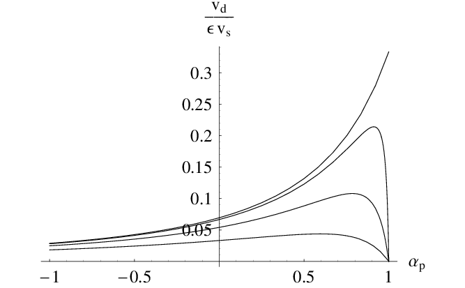
Figure 2 shows as a function of for a variety of values of .

A striking feature of figure 2 is that the maximum of occurs at a positive value of , so positive persistence increases (up to a point). This is markedly different to the case of a cell responding to the instantaneous chemoattractant concentration gradient (the case analysed by Schnitzer 1993), for which is highest for . Figure 3 compares the two cases. A qualitative explanation of the enhancement of by persistence for a cell performing temporal comparisons is as follows. Inspection of (2) reveals that the largest modulations in occur when the cell swims straight up or down the concentration gradient for or more. For larger , the cell is more likely to swim approximately straight up or down the gradient for or more (since it undergoes a smaller change of direction when it tumbles), hence is on average modulated by a larger amount, and on average the chemotactic response is stronger. Alternatively, one can explain the effect in terms of the relevance of past concentration information. If is close to 1, then information about the concentration over the last , on the basis of which the cell biases its tumble rate, is more relevant than if .
Figure 2 also shows that for , as . This makes sense intuitively since for the cell effectively does not tumble at all and hence is unable to bias its random walk. However, for it appears that is largest when , whereas sensibly one expects that when . This apparent paradox can be resolved if one considers the time-scales over which our results are valid. In deriving (37), we assumed that the probability distribution governing is steady state. This is true only if the cell has been swimming in the chemoattractant gradient for a time , where the direction correlation time is given by (26). For , tumbles and rotational Brownian motion have randomised the cell’s swimming direction so that the current swimming direction is independent of any initial conditions. Clearly as for , so , is singularity at which our results are not valid.
The observed persistence in wild-type E. coli is (Berg 1983), and (57) predicts that for a rotational diffusivity of , is larger for than for . Thus, wild-type E. coli cells enhance their drift velocity considerably by having non-zero persistence. However, the drift velocity is maximised by a persistence of , which is considerably larger than the observed persistence of . This discrepancy seems surprising, since one might expect evolution to have optimised to maximise . One possible explanation for the discrepancy is a compromise between transient and steady-state behaviours of the cell. Clark and Grant 2005 suggested that in order for a bacterium to be successful it must both both (a) move toward nutrients in the short run (maximise ) and (b) in the long run spend most of its time near the regions of highest nutrient density if confined to a bounded domain. Clark and Grant 2005 argued that the double lobed form of can be understood in terms of a compromise between (a) and (b), with (a) favouring an with only a positive lobe and (b) favouring an with only a negative lobe. A similar compromise may govern .
Steady state performance is optimised by an close to zero, for the following reason. The translational self-diffusion coefficient of a cell performing runs and tumbles is (Lovely and Dahlquist 1975) and, from (26), is a monotonically increasing function of . Now, suppose a cell is confined to a bounded domain with uniform . Ideally, in the long term, the cell would spend all its time right at the boundary with the highest . In fact, the cell wanders within a characteristic length of that boundary, where is governed by a balance between diffusion away from the boundary and drift velocity toward the boundary. For , one can show that is minimised by . A similar argument holds if one considers a distribution of chemoattractant with a local maximum, with the same conclusion that long term performance is optimised by close to zero. Thus, the observed persistence of might reflect a compromise between transient and steady-state performance.
A second factor that disfavours large is that E. coli are denser than water, which may cause them to eventually swim downward in the absence of strong tumbles. For instance, Salmonella typhimurium is a denser-than-water bacterium that performs run and tumble chemotaxis in a similar manner to E. coli, and mutant non-tumbling S. typhimurium cells swim downward on average and collect at the bottom of the vessel in which they are contained (Aswad and Coshland 1975). This is presumably because the hydrodynamic drag on the flagella is larger than that on the cell body, so a torque is exerted on a non-vertically-oriented cell (Roberts and Deacon 2002). The implication is that it would be disadvantageous for a cell to have very close to since it would then swim downward on average, regardless of the direction of the chemoattractant gradient.
Other factors potentially influencing the optimal value of for a real E. coli cell are that (i) an environment with background fluid flows or with rapidly changing distributions of nutrients may favour a smaller , so that the cell may perform a ‘U-turn’ more quickly, and that (ii) non-linear effects have been neglected in our analysis and may play an important role for in its native environment.
6 Confirmation of results by Monte Carlo simulation
Monte Carlo simulation was used to verify the correctness of the analytic calculations for and to assess the accuracy of the analytic calculations for larger . For the purpose of simulations, we used a different response function:
| (58) |
This form of was chosen for computational convenience; only the most recent four seconds of a cell’s trajectory need to be stored in memory. Like the defined by (56), the defined by (58) possesses a positive lobe followed by a negative lobe of equal area, and . Note that we do not have to specify a value for , since and appear together as a product in the equation for .
The simulation method was as follows. For each set of parameter values, 100 simulations were run, each simulating of swimming. Time was discretised into steps of size . At each time-step, the tumble probability was calculated using a discrete approximation of the integral (2), and a random number generator was used to decide whether the cell tumbled. If the cell tumbled, then the new direction faced after the tumble was chosen from an axisymmetric distribution about the old direction, such that the new direction made an angle of with the old direction. If the cell didn’t tumble, then rotational Brownian motion was simulated by giving the cell a new direction chosen from an axisymmetric distribution about the old direction, such that the new direction made an angle of with the old direction (note that this is consistent with equation 17). For each simulation, the drift velocity was estimated as the net displacement divided by the simulation duration. The baseline tumble rate was set to for all simulations.


For , there is excellent agreement between the simulation data and analytic calculations, as shown in figure 4. For larger , the accuracy of the analytic calculations is diminished. Figure 5 shows that the results of the analytic calculations are within of the simulation results for up to approximately .
7 Discussion and Conclusion
In this paper we presented an analytic method for calculating the drift velocity of a cell performing run and tumble chemotaxis, taking account of (i) temporal comparisons, (ii) persistence, and (iii) rotational Brownian motion, and we verified the results with Monte Carlo simulations. The calculations are novel in that they are the first calculation of chemotactic drift velocity simultaneously to include all features (i), (ii) and (iii) of the motion. Using estimates for the chemotactic response function and the rotational diffusivity, our key finding is that persistence can markedly increase the drift velocity. For instance, a persistence of (characteristic of wild-type E. coli (Berg 1983)) can increase the drift velocity by relative to , while a persistence of can double the drift velocity relative to .
There are a number of possible reasons for discrepancy between the value of that maximises and the value of observed in wild-type E. coli. First, our model looks only at behaviour in an unbounded domain, or equivalently at transient behaviour in a bounded domain, whereas one expects that in order to be successful a bacterium must optimise both its transient and its steady state behaviour. Indeed, it has been proposed that the double-lobed form of reflects a compromise between transient and steady state behaviour (Clark and Grant 2005). The same might be true of , with a smaller value of resulting in a more favourable steady-state behaviour. Second, our analysis neglects the fact that E. coli cells are denser than the fluid in which they swim and geometrically asymmetric (front-to-back), so that a cell with would swim downward on average. Third, our analysis does not include rapidly varying chemoattractant distributions or background fluid flows. Finally, our analysis is linear and therefore limited to weak chemoattractant gradients; it is not inconceivable that the dependence of drift velocity on persistence might be different in stronger chemoattractant gradients.
Acknowledgements.
I would like to thank Professor Tim Pedley for his guidance and encouragement, Dr Kalvis Jansons for his advice on notation, and Professor Howard Berg for fruitful conversations.References
- Aswad and Coshland (1975) Aswad D, Coshland DE (1975) Isolation, characterization and complementation of Salmonella typhimurium chemotaxis mutants. J Mol Biol 97(2):225–235
- Berg (1983) Berg HC (1983) Random Walks in Biology. Princeton University Press
- Berg and Brown (1972) Berg HC, Brown DA (1972) Chemotaxis in Escherichia coli analysed by three-dimensional tracking. Nature 239:500–504
- Block et al (1982) Block SM, Segall JE, Berg HC (1982) Impulse responses in bacterial chemotaxis. Cell 31:215–226
- Brown and Berg (1974) Brown DA, Berg HC (1974) Temporal stimulation of chemotaxis in Escherichia coli. Proc Nat Acad Sci USA 71(4):1388–1392
- Clark and Grant (2005) Clark DA, Grant LC (2005) The bacterial chemotactic response reflects a compromise between transient and steady-state behavior. Proc Nat Acad Sci USA 102(26):9150–9155
- de Gennes (2004) de Gennes PG (2004) Chemotaxis: the role of internal delays. Eur Biophys J 33:691–693
- Erban and Othmer (2005) Erban R, Othmer HG (2005) From signal transduction to spatial pattern formation in E. coli: a paradigm for multiscale modeling in biology. Multiscale Model Simul 3(2):362–394
- Lovely and Dahlquist (1975) Lovely PS, Dahlquist FW (1975) Statistical measures of bacterial motility and chemotaxis. J Theor Biol 50:477–496
- Patlak (1953) Patlak CS (1953) Random walk with persistence and external bias. Bull Math Biophys 15:311–338
- Roberts and Deacon (2002) Roberts AM, Deacon FM (2002) Gravitaxis in motile micro-organisms: the role of foreaft body asymmetry. J Fluid Mech 452:405–423
- Schnitzer (1993) Schnitzer MJ (1993) Theory of continuum random walks and applications to chemotaxis. Phys Rev E 48(4):2553–2568
- Segall et al (1982) Segall JE, Manson MD, Berg HC (1982) Signal processing times in bacterial chemotaxis. Nature 296:855–857
- Segall et al (1986) Segall JE, Block SM, Berg HC (1986) Temporal comparisons in bacterial chemotaxis. Proc Nat Acad Sci USA 83(23):8987–8991
Appendix A Solving the Fokker-Planck equation
The Fokker-Planck equation is
| (59) |
where is the Laplacian in direction space and is the swimming direction. We can describe by spherical polar coordinates, so that and is the probability that lies in the solid angle . Assume axisymmetry, so that is a function of only. Writing out the Laplacian in full, we then have
| (60) |
Without loss of generality, we choose our initial condition to be . Since we are only interested in the direction correlation function, we need only calculate rather than solve for . Consider
| (61) |
Substituting (60) into (61) and integrating by parts, one finds
| (62) |
so
| (63) |
Generalising from this result it is straightforward to show that
| (64) |