Daily Observations of Interstellar Scintillation in PSR B0329+54
Abstract
Quasi-continuous observations of PSR B0329+54 over 20 days using the Nanshan 25-m telescope at 1540 MHz have been used to study the effects of refractive scintillation on the pulsar flux density and diffractive scintillation properties. Dynamic spectra were obtained from datasets of 90 min duration and diffractive parameters derived from a two-dimensional auto-correlation analysis. Secondary spectra were also computed but these showed no significant evidence for arc structure. Cross correlations between variations in the derived parameters were much lower than predicted by thin screen models and in one case was of opposite sign to the prediction. Observed modulation indices were larger than predicted by thin screen models with a Kolmogorov fluctuation spectrum. Structure functions were computed for the flux density, diffractive timescale and decorrelation bandwidth. These indicated a refractive timescale of h, much shorter than predicted by the thin screen model. The measured structure-function slope of is also inconsistent with scattering by a single thin screen for which a slope of 2.0 is expected. All observations are consistent with scattering by an extended medium having a Kolmogorov fluctuation spectrum which is concentrated towards the pulsar. This interpretation is also consistent with recent observations of multiple diffuse scintillation arcs for this pulsar.
Keywords:
pulsars:individual:PSR B0329+54 – ISM:structure1 Introduction
In the early days of pulsar observations, slow fluctuations of pulsar amplitudes were reported by Cole et al. 1970 and Huguenin et al. 1973. But it was not recognized that they were an interstellar propagation effect until a close correlation between the time-scale of the intensity fluctuations and the pulsar dispersion measure was pointed out by Sieber 1982. Subsequently, Rickett et al. 1984 explained these slow fluctuations as refractive interstellar scintillations (RISS). This phenomenon is produced by the same spectrum of electron density fluctuations in the interstellar medium that is responsible for the well known diffractive scintillation (DISS). DISS is caused by the small spatial scale density fluctuations ( m) and it appears as intensity variations in both the time and frequency domains with characteristic scales of minutes to hours and kHz to MHz respectively. On the other hand, large-scale inhomogeneities ( m) in the interstellar medium give rise to focussing effects observed as RISS. A good review of the theory behind this interpretation is given by Rickett 1990.
It is generally accepted that the spectrum of electron density fluctuations in the interstellar medium has a power-law form:
| (1) |
where is the wave-vector associated with a spatial size . The quantity is a measure of turbulence along a particular line of sight. The power-law index which indicates the steepness of the inhomogeneity spectrum is in the range of . But the details of the spectrum, e.g. its slope and the range of scale sizes over which it is valid, still remain open questions. Also, different assumptions are made about the distribution of scattering material along the path to the pulsar. Many observations are well accounted for by models in which the scattering is concentrated in a single centrally located thin screen, but others imply that there are many scattering sites or a statistically uniform screen extending over most or all of the path.
A range of observations suggest that a Kolmogorov fluctuation spectrum with is widely applicable in the interstellar medium (Armstrong et al. 1995). However, observational studies showing, for example, persistent drifting bands in dynamic spectra and increased modulation of diffractive properties suggest that excess power is often seen at low spatial frequencies, implying a spectral index . Examples of extensive studies are those by Gupta et al. 1994, who studied eight pulsars at 408 MHz using the Lovell telescope and interpreted changing diffractive patterns in dynamic spectra in terms of refractive effects, and those by Bhat et al. 1999a; Bhat et al. 1999b and Bhat et al. 1999. These latter authors used the Ooty radio telescope at 327 MHz to study 18 pulsars over a 2.5-year dataspan and showed that, while many observations were consistent with a Kolmogorov spectrum, others showed evidence of a steeper spectrum. Stinebring et al. 2000 reported on 5 years of daily monitoring of the flux density of 21 pulsars at 610 MHz, showing that most of the results, covering a wide range of scattering strengths, were consistent with a Kolmogorov fluctuation spectrum. In some pulsars, though modulation indices were higher than expected, possibly due to the presence of an “inner scale”, a cutoff in the fluctuation spectrum at scales greater than the diffractive scale , where is the wavelength and is the angular size of the scattering disk.
Other observations suggesting steeper power-law spectra () include fringing in dynamic spectra implying multiple imaging (Cordes et al. 1986; Cordes & Wolszczan 1986; Rickett et al. 1997, e.g.,) and extreme scattering events (Lestrade et al. 1998). Blandford & Narayan 1985 suggested a steeper spectrum to deal with the theoretical difficulties in supporting a turbulent cascade in the Kolmogorov spectrum. Based on power-law models of the spectrum, Romani et al. 1986 analysed the effects of RISS on diffractive parameters for different slopes , 4 and 4.3, predicting anti-correlations for (,) and (, ), where is flux density and , are the diffractive scintillation bandwidth and timescale, respectively and a postive correlation for (,), with the magnitudes of the correlation coefficients being larger for steeper spectra.
More recent observations have tended to concentrate on detailed studies of individual pulsars (Shishov et al. 2003; Ramachandran et al. 2006; Smirnova et al. 2006, e.g.,) or on the fascinating “scintillation arcs” which are seen in secondary spectra, that is, two-dimensional Fourier transforms of dynamic spectra, in high-sensitivity, high-resolution observations (Stinebring et al. 2001; Hill et al. 2003; Stinebring 2006). These arcs, which are closely related to multiple imaging and the frequently observed “criss-cross” sloping bands, result from interference between rays in a central core and rays from an extended scattering disk. They form a powerful probe of structure in the interstellar medium (Cordes et al. 2006). For example, Putney & Stinebring 2006 present recent observations of six pulsars showing multiple arcs of different curvature implying a distribution of scattering centres along the line of sight.
PSR B0329+54 is one of the strongest pulsars known and its scintillation properties have been studied by many authors. Observations at 610 MHz by Stinebring et al. 1996 showed that the correlations between variations of flux, decorrelation bandwidth and scintillation time-scale were consistent with the theoretical predictions with . However, Bhat et al. 1999b found that for PSR B0329+54, correlations between these parameters at 327 MHz were not in accord with the predictions. Long-term flux density monitoring at 610 MHz by Stinebring et al. 2000 showed that the modulation index was somewhat higher than expected for a Kolmogorov spectrum, i.e. . Shishov et al. 2003 took data obtained over a wide range of frequencies finding a value of , less than but consistent with a Kolmogorov turbulence spectrum, and interpreted this result in terms of weak plasma turbulence in the interstellar medium. Observations at 1540 MHz using the Nanshan telescope (Wang et al. 2005) showed inconsistencies in values of the power-law index obtained from two different approaches. The ratio of refractive scattering angle and diffractive angle gave , while the frequency dependence of scintillation parameters gave . These conflicting results suggested undertaking observations with a better sampling of the refractive variations. These have a predicted timescale
| (2) |
(Gupta et al. 1993; Stinebring et al. 2000), about four days for this pulsar.
In this paper, we present the results of quasi-continuous 1540 MHz observations of PSR B0329+54 over a 20-day interval in 2004, March. Diffractive parameters were sampled at 90-min intervals, giving good resolution of the expected RISS variations. The layout for the rest of this paper is as follows: in Section 2 we introduce the observations; data analysis and results are shown in Section 3, and in Section 4, we discuss the results and their interpretation. Conclusions are presented in Section 5.
2 Observations
The observations were made using the Nanshan 25 m radio telescope with a central frequency of 1540 MHz. Our system is sensitive to orthogonal linear polarizations and the system temperature for the two channels is 20 K and 22 K respectively. Each polarization has 128 channels, each of bandwidth 2.5 MHz, giving a total bandwidth of 320 MHz. After detection and high-pass filtering, the data are 1-bit sampled and folded at the apparent pulsar period. Signals from the two polarizations are summed to form total intensity pulse profiles.
We made our observations from March 12 to March 31 in 2004, and obtained more than 150 scintillation dynamic spectra for PSR B0329+54. The observations were continuous (PSR B0329+54 is circumpolar at Nanshan) apart from an interruption of about 3 days from March 20 due to telescope problems. In our analysis, the time block for each dynamic spectrum is typically 90 minutes with a sub-integration time of 60 s. We calibrated the pulsar flux density scale using observations of ten strong, relatively distant pulsars which all have well-measured flux densities in the ATNF pulsar catalogue (www.atnf.csiro.au/research/pulsar/psrcat).
3 Data Analysis and Results
3.1 Scintillation Dynamic Spectra
Dynamic spectra were obtained for each observation by plotting the mean flux density in each channel against time. Examples of these plots are shown in Fig. 1. Channels badly affected by radio-frequency interference have been interpolated over from adjacent frequency channels.

Fig. 1 shows that the dynamic spectra are well resolved and that the scintles or peaks of flux density change their shapes and sizes in the frequency and time domains. At some epochs, the pulsar seems weaker and the scintles are smaller (MJD 53088.4), and at other epochs, the pulsar signal is stronger and the scintles larger (e.g. MJDs 53081.6, 53083.2, 53093.3). The frequency dependence of DISS can be seen within our receiver bandwidth, i.e., scintles are smaller at the lower end of the observed band (MJD 53091.8). At some epochs the spectra show a significant drifting pattern (e.g. MJD 53082.4), which implies a modulation by RISS. However, we didn’t observe the fine fringes seen in the data of Wang et al. 2005. The scintles are generally smaller in this observing session, resulting in a smaller value in , which we will discuss more in Section 3.4. Deep modulations are common in all the dynamic spectra we have recorded.
The limited number of scintles in the dynamic spectra introduces a statistical estimation error in the scintillation parameters (Cordes et al. 1985). An approximate estimate of the number of scintles in the dynamic spectra is given by:
| (3) |
where is the total observing time and the total observing bandwidth, decorrelation bandwidth and is the DISS timescale. The fractional estimation error is then given by:
| (4) |
where we assume a scintle filling factor of 0.5 (Bhat et al. 1999a). This error contribution is taken into account in the estimates of scintillation parameters in Section 3.4.
3.2 Secondary Spectrum
The two-dimensional Fourier spectrum of the primary dynamic spectrum is often referred to as the secondary spectrum. To show the beautiful arc structures (Stinebring 2006, e.g.,), high frequency resolution and high sensitivity are required. Unfortunately, the Nanshan system does not provide these. However, earlier observations at 1540 MHz for this pulsar by Wang et al. 2005 showed sloping fringes in the dynamic spectra resulting in offset features in the secondary spectra. Surprisingly, despite using the same system at Nanshan, our three-week consecutive observations show no significant arc structure or offset features in the secondary spectra.
3.3 Two-Dimensional Auto-Correlation Function
To quantify the diffractive parameters, we use the two-dimensional auto-correlation function (ACF), which was computed for frequency lags up to half of the observing bandwidth and for time lags up to half of the observing time. The ACF of the dynamic spectra is defined as:
| (5) |
where , and is the mean pulsar flux density over each observation, then the normalized ACF is:
| (6) |

We plot the normalized ACF and one dimensional cut at zero time and frequency lag in Fig. 2. These figures correspond to the dynamic spectra shown in Fig. 1. Following convention, the DISS time-scale is defined as the time lag at zero frequency lag where the ACF is 1/e of the maximum, and the decorrelation bandwidth is defined as the half-width at half-maximum of the ACF along the frequency lag axis at zero time lag (Cordes 1986). For weaker pulsars, random system noise results in a strong spike at the zero time and frequency lag of ACF. For PSR B0329+54 the spike is weak but still observable at some epochs. To remove the spike at the origin we used the four neighbouring frequency-lag points to fit for a parabola across the zero frequency lag. The central point is interpolated from this fit.
3.4 ACF and Scintillation Parameters
Following Gupta et al. 1994 and Bhat et al. 1999a, we use a two-dimensional elliptical Gaussian function to fit the ACF with form:
| (7) |
in which is unity since the ACF is normalized to unity. By using a minimization procedure, we obtained parameters , and . The fitting procedure was a search for the three non-linear parameters for the least-squared error between model and data over the central region of ACF. The scintillation parameters and are calculated as:
| (8) | ||||
| (9) |
Following Bhat et al. 1999a, we use to describe the orientation of the elliptical Gaussian. This is proportional to the refractive scattering angle , and is given by:
| (10) |
.
From the analysis, we also obtained the uncertainties for , and . Using these uncertainties added in quadrature with the statistical error (Equation 4), we calculate the errors of , and . Since has zero mean, we applied the statistical error to rather than to itself. For flux density, measurement errors are estimated from the baseline noise in the mean pulse profiles. Time variations of , , and along with their uncertainties are shown in Fig. 3. These parameters show significant variations with time which can be explained as an RISS effect as discussed in Section 4.

3.5 Derived Scattering Parameters
Given a power-law spectrum of electron density fluctuations (Equation 1), the average scattering level along the line-of-sight, , for a Kolmogorov spectrum is given by
| (11) |
Another quantitative measurement of the strength of scattering is the parameter which is defined as the ratio of the Fresnel scale to the coherence scale (Rickett 1990), where is the diffractive scattering angle. For strong scattering, . In terms of the diffractive scintillation parameter :
| (12) |
The diffractive timescale depends on the velocity of the ray path across the scattering screen. Assuming a thin screen and that the pulsar velocity dominates, an estimate for the pulsar transverse velocity based on the scintillation parameters is:
| (13) |
where is the ratio of the observer-screen distance to the pulsar-screen distance and the proportionality constant (Gupta et al. 1994).
In Table 1 we give some basic parameters for the pulsar and observations as well as mean values for the basic scattering parameters. The pulsar distance is based on a parallax measurement by Brisken et al. 2002 who also measured the pulsar proper motion, mas yr-1 which, with the distance, gives the transverse velocity listed in the table. The typical observation time for each dynamic spectrum and the total number of such observations are given.
| Galactic longitude (deg) | 145.00 |
|---|---|
| Galactic latitude (deg) | |
| DM (pc cm-3) | 26.83 |
| Distance (kpc) | |
| (km s-1) | |
| Observation time (min) | 90 |
| Number of observations | 168 |
| (MHz) | |
| (min) | |
| () | |
| (h) | |
| () | |
| (km s-1) |
In the lower part of the table we give the mean values and rms scatter for the decorrelation bandwidth (), scintillation time-scale () and the slope parameter () derived from the ACF analysis. We note that the scintillation timescale is much less than the observation time (90 min), so the effects of finite observation time discussed by (Stinebring et al. 2000) should be minimal. The predicted refractive timescale, based on the diffractive parameters (Equation 2), is about 4 d, but the observed value (Section 4.4) is much less than that. The derived scattering level, , and scattering strength, , both indicate that scattering is strong along the path to PSR B0329+54. For the quoted scintillation velocity, a centrally located screen () has been assumed. Our value is somewhat lower than the proper motion velocity. It is much lower than the value given for this pulsar by Gupta et al. 1994 based on 408 MHz observations, but they assumed a pulsar distance of 2.3 kpc. For the parallax distance of kpc, their velocity becomes km s-1, consistent with the proper motion velocity. From their 327 MHz observations Bhat et al. 1999a derive a scintillation velocity of km s-1 based on an assumed pulsar distance of 1.43 kpc. Scaled with the parallax distance, this becomes km s-1. While these results are not too discordant, it is clear that there are variations on timescales much longer than the nominal refractive time and also that the frequency scaling of the diffractive parameters does not precisely follow the Kolmogorov prediction (Wang et al. 2005, cf.).
4 Interpretation of Results
4.1 Cross-Correlations Between Scintillation Parameters
Romani et al. 1986 suggested that correlations should exist between variations of the flux density , decorrelation bandwidth , and diffractive timescale . These predictions assume a single-phase screen and a simple power-law description for the electron density fluctuations. In Table 2 we list the predicted correlation coefficients for turbulence spectra of 11/3, 4 and 4.3 (Romani et al. 1986).
| {, } | {, } | {, } | ||
| RNB86 | ||||
| SFM96 | ||||
| Spearman | ||||
| BRG99b | Spearman | |||
| This work | Spearman | |||
| 95% confidence interval |
Stinebring et al. 1996 and Bhat et al. 1999b studied the correlations between the variations of , and for PSR B0329+54. Both papers use the Spearman rank-order correlation coefficient () to describe the correlation between the parameters. is given by:
| (14) |
where and are the ranks of the two quantities and for which the correlation coefficient is computed and the summation is carried out over the total number of the data points. and represent the average values of and . This method is less sensitive to the outlying points than the usual correlation coefficient , which is computed with the same equation but with the actual data values rather than their rank. and its confidence interval are derived using the ‘bootstrap’ method as follows: assume we have an original object O with a set of N elements. We construct a new list with the same number of N elements from the original list by randomly picking elements from the list. Any one element from the list can be picked any number of times. The process is repeated 10000 times to give new series {, ….} from which we obtain a statistical distribution of . The mean value and 95% confidence limits are derived from this distribution.
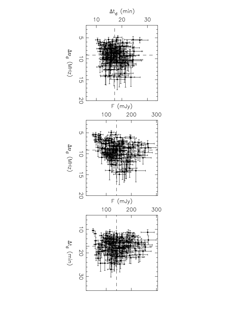
The results for are presented in Table 2, along with results from Stinebring et al. 1996 and Bhat et al. 1999b for comparison.
Although Stinebring et al. 1996 found significant cross-correlations between the scintillation parameters which were approximately in accord with the theoretical predictions, neither Bhat et al. 1999b nor our observations show such correlations. As Fig. 4 shows, little or no correlation is observed between and and the correlation between and even has the opposite sign to the theoretical prediction. In contrast to the other studies, we observe only a very weak correlation between and . The observed correlations are clearly not well described by the thin-screen model of Romani et al. 1986. Their predictions are not strongly dependent on the assumed slope of the fluctuation spectrum so other factors, for example, an extended scattering region, must be important. However, there have been no predictions for the expected correlations in this case.
4.2 Structure function analysis
We use a structure function analysis to study the refractive variations in the flux density and the diffractive timescale and decorrelation bandwidth. The structure function is defined to be:
| (15) |
where is the structure function at lag of n units of the observation time (90 min), is the flux density value for the th observation, if exists and zero otherwise, is the mean flux density, and is the number of products in for which . Typically, the structure function has three regimes: a noise regime at small lags, a structure regime characterized by a linear slope on a log-log plot and a saturation regime where it flattens out at large lags. The shape of the structure function may be used to derive the refractive modulation index and the refractive scintillation time-scale . The modulation index is expressed as , where is the saturation value of the structure function, and the refractive time-scale is the time lag at which the structure function reaches half of its saturation value. The logarithmic slope of the structure function, , is defined in the linear structure region. Structure functions for the refractive variations in diffractive timescale and bandwidth may be similarly defined.
Structure functions must be corrected for the effects of noise in the time series. The noise contribution to the structure function values, , where is the statistical estimation error resulting from the finite number of scintles in the dynamic spectrum (Equation 4), is the mean fractional uncertainty in the measured parameter. In Table 3 we list measured values of , , and for the three quantities, along with the uncorrected value of , the 90-min lag value. Corrected values of the derived structure functions, that is, with subtracted, are shown in Fig. 5. Uncertainties on the structure function values are given by (Stinebring & Condon 1990). In all cases, the corrected value of is below the extrapolation of the linear part of the structure function, indicating that we may have somewhat over-estimated the noise contribution.
| Parameter | |||||
|---|---|---|---|---|---|
| 0.045 | 0.110 | 0.119 | 0.028 | 0.065 | |
| 0.058 | 0.110 | 0.124 | 0.030 | 0.065 | |
| 0.058 | 0.110 | 0.124 | 0.030 | 0.041 |
 |
 |
 |
4.3 Modulation Indices of Scintillation Parameters
In strong scattering, the diffractive parameters are modulated by refractive effects. Romani et al. 1986 gave relations for the expected modulation indices for refractive variations of flux density (), diffractive bandwidth () and diffractive timescale () for power-law fluctuation spectra with , 4 and 4.3. For the steeper spectra, the modulation indices are largely independent of scattering strength and frequency. They found that the depth of modulation is lowest for the Kolmogorov spectrum and larger for larger values of . Predicted modulation indices for PSR B0329+54 are given in columns 2 – 4 of Table 4 . Based on the Romani et al. 1986 theory, Bhat et al. 1999 gave the modulation indices of , , and for and . We list them in column 3 & 4 of Table 4.
The noise-corrected modulation indices may be computed directly from the time series using
| (16) |
where is the observed rms fluctuation relative to the mean. The modulation index has an uncertainty given by
| (17) |
where is approximately the data span divided by the refractive timescale and is the number of independent observations. Using the noise estimates given in Table 3, the derived modulation indices and their uncertainties are given in column 5 of Table 4. The derived values are consistently larger than the predicted values for a Kolmogorov spectrum (Stinebring et al. 2000, cf.), indicating a .
| Prediction | Our | |||
|---|---|---|---|---|
| Observation | ||||
| 0.22 | 0.38 | 0.55 | ||
| 0.15 | 0.35 | 0.57 | ||
| 0.07 | 0.17 | 0.25 |
Another possible intepretation of the relatively large observed modulation indices is that the scattering medium is extended so that the thin-screen approximation is not valid. The flux density modulation index for a statistically uniform scattering medium with a Kolmogorov spectrum () covering the whole path to the pulsar has been discussed by Coles et al. 1987, Gupta et al. 1993, Stinebring et al. 2000 and Smirnova et al. 1998 with the result
| (18) |
For our observations of PSR B0329+54, this relation gives a predicted , larger than the observed value. This implies that, as an alternative to a steeper spectrum, the observed modulation index could be accounted for by an extended Kolmogorov scattering medium covering just part of the path.
4.4 Refractive Timescales
The horizontal dashed lines on the structure function plots (Fig. 5) are at , where is the observed modulation index given in in Table 4. The refractive timescale is defined to be the lag at which the structure function falls to . In the flux density case, this is at h. The structure functions for the diffractive bandwidth and timescale are less well defined, but clearly also imply a short refractive timescale. The measured timescale is much less than the predicted value of about 96 h based on a central thin-screen model and the observed diffractive timescale (Table 1). For an extended scattering medium with a Kolmogorov spectrum, evaluating the equations of Smirnova et al. 1998 with practical units gives
| (19) |
Substituting the parameters from our observations of PSR B0329+54 gives a value of about 32 hours, again much larger than the observed value.
Smirnova et al. 1998 also consider the case of a thin screen at an arbitrary location along the path and show that is proportional to the pulsar-screen distance () whereas is proportional to . Therefore, if , refractive times are much reduced, whereas is only weakly dependent on . This breaks the approximate proportionality of and (Equation 2) which applies to both a central thin screen and an extended medium. The scintillation arc observations of Putney & Stinebring 2006 suggest that most of the scattering for PSR B0329+54 occurs relatively close to the pulsar, supporting this interpretation of the short refractive timescale.
4.5 Structure Function Slope
The slope of the linear part of the structure function, between the noise and saturation regimes, is related to the power-law index of the fluctuation spectrum. For a single thin screen, the slope should be 2.0 for (Romani et al. 1986; Smirnova et al. 1998). For an extended screen, the predicted slope is (Smirnova et al. 1998). Although the observed slopes are not very well determined, they are clearly . The measured value for the flux density structure function slope is and the values for the other two structure functions are similar. This is clearly inconsistent with scattering by a single thin screen. As we have argued above, there are good arguments supporting the idea that the scattering screen in this direction is extended; in this case, the implied value of , somewhat less than but marginally consistent with the Kolmogorov value. Based on the thin-screen model, observed diffractive bandwidths and a refractive interpretation of band slopes (), Bhat et al. 1999a and Wang et al. 2005 also obtain values less than the Kolmogorov value for PSR B0329+54 and several other pulsars. Our result also agrees well with that from Stinebring et al. 2000 who obtain a structure function slope of from their flux density monitoring of this pulsar. However, it contrasts with that of Shishov et al. 2003 where a structure function slope is derived from observations at several different frequencies and interpreted in terms of weak plasma turbulence, again with a Kolmogorov spectrum.
5 Conclusions
Quasi-continuous observations of PSR B0329+54 at 1540 MHz over 20 days have been analysed to investigate the refractive modulations of the pulsar flux density and diffractive scintillation parameters. The data set was split into more than 150 individual observations, each of 90-min duration, and two-dimensional auto-correlations and secondary spectra computed. Time series of the pulsar flux density (), decorrelation bandwidth (), diffractive scintillation time-scale () and drift rate of features in the dynamic spectra () clearly show refractive modulation, although no evidence for arc structure is seen in the secondary spectra.
Observed cross-correlations between variations in the flux density and diffractive parameters were much smaller than predictions based on the thin-screen model. In one case the sign of the correlation was opposite to the predicted value. Similar results have been obtained by other observers although different observations appear to give conflicting results.
In accordance with previous work, observed modulation indices are greater than predicted for a thin screen with a Kolmogorov fluctuation spectrum. This could be accounted for either by a steeper fluctuation spectrum () or by scattering in an extended medium. The predicted modulation index for a scattering medium covering the whole path to the pulsar is greater than that observed, suggesting that the scattering medium, while extended, does not cover the whole path. Structure functions derived from the observations indicate a short refractive timescale, h, much less than predicted from the thin screen model, and have a relatively flat slope, , again inconsistent with scattering by a thin screen.
The observed modulation indices, structure function slopes and short refractive timescales all are consistent with scattering by an extended region with a Kolmogorov fluctuation spectrum which is concentrated toward the pulsar. This idea is supported by recent high-sensitivity observations of PSR B0329+54 by Putney & Stinebring 2006 which show indistinct scintillation arcs corresponding to extended scattering regions relatively close to the pulsar.
Acknowledgments
We would like to thank B. J. Rickett and W. A. Coles for helpful discussions. This work is supported by the Key Directional Project of CAS and NNSFC under the project 10173020 and 10673021.
References
- Armstrong et al. (1995) Armstrong J. W., Rickett B. J., Spangler S. R., 1995, ApJ, 443, 209
- Bhat et al. (1999) Bhat N. D. R., Gupta Y., Rao A. P., 1999, ApJ, 514, 249
- Bhat et al. (1999a) Bhat N. D. R., Rao A. P., Gupta Y., 1999a, ApJS, 121, 483
- Bhat et al. (1999b) Bhat N. D. R., Rao A. P., Gupta Y., 1999b, ApJ, 514, 272
- Blandford & Narayan (1985) Blandford R. D., Narayan R., 1985, MNRAS, 213, 591
- Brisken et al. (2002) Brisken W. F., Benson J. M., Goss W. M., Thorsett S. E., 2002, ApJ, 571, 906
- Cole et al. (1970) Cole T. W., Hesse H. K., Page C. G., 1970, Nature, 225, 712
- Coles et al. (1987) Coles W. A., Frehlich R. G., Rickett B. J., Codona J. L., 1987, ApJ, 315, 666
- Cordes (1986) Cordes J. M., 1986, ApJ, 311, 183
- Cordes et al. (1986) Cordes J. M., Pidwerbetsky A., Lovelace R. V. E., 1986, ApJ, 310, 737
- Cordes et al. (2006) Cordes J. M., Rickett B. J., Stinebring D. R., Coles W. A., 2006, ApJ, 637, 346
- Cordes et al. (1985) Cordes J. M., Weisberg J. M., Boriakoff V., 1985, ApJ, 288, 221
- Cordes & Wolszczan (1986) Cordes J. M., Wolszczan A., 1986, ApJ, 307, L27
- Gupta et al. (1993) Gupta Y., Rickett B. J., Coles W. A., 1993, ApJ, 403, 183
- Gupta et al. (1994) Gupta Y., Rickett B. J., Lyne A. G., 1994, MNRAS, 269, 1035
- Hill et al. (2003) Hill A. S., Stinebring D. R., Barnor H. A., Berwick D. E., Webber A. B., 2003, ApJ, 599, 457
- Huguenin et al. (1973) Huguenin G. R., Taylor J. H., Helfand D. J., 1973, ApJ, 181, L139
- Lestrade et al. (1998) Lestrade J., Rickett B. J., I. C., 1998, A&A, 334, 1068
- Putney & Stinebring (2006) Putney M. L., Stinebring D. R., 2006, Chin. J. Atron. Astrophys., Suppl. 2, 6, 233
- Ramachandran et al. (2006) Ramachandran R., Demorest P., Backer D. C., Cognard I., Lommen A., 2006, ApJ, 645, 303
- Rickett (1990) Rickett B. J., 1990, Ann. Rev. Astr. Ap., 28, 561
- Rickett et al. (1984) Rickett B. J., Coles W. A., Bourgois G., 1984, A&A, 134, 390
- Rickett et al. (1997) Rickett B. J., Lyne A. G., Gupta Y., 1997, MNRAS, 287, 739
- Romani et al. (1986) Romani R. W., Narayan R., Blandford R., 1986, MNRAS, 220, 19
- Shishov et al. (2003) Shishov V. I., Smirnova T. V., Sieber W., Malofeev V. M., Potapov V. A., Stinebring D., Kramer M., Jessner A., Wielebinski R., 2003, A&A, 404, 557
- Sieber (1982) Sieber W., 1982, A&A, 113, 311
- Smirnova et al. (2006) Smirnova T. V., Shishov V. I., Sieber W., Stinebring D. R., Malofeev V. M., Potapov V. A., Tyul’Bashev S. A., Jessner A., Wielebinski R., 2006, A&A, 455, 195
- Smirnova et al. (1998) Smirnova T. V., Shishov V. I., Stinebring D. R., 1998, Astron. Reports, 42, 766
- Stinebring (2006) Stinebring D. R., 2006, Chin. J. Atron. Astrophys., Suppl. 2, 6, 204
- Stinebring & Condon (1990) Stinebring D. R., Condon J. J., 1990, ApJ, 352, 207
- Stinebring et al. (1996) Stinebring D. R., Faison M. D., McKinnon M. M., 1996, ApJ, 460, 460
- Stinebring et al. (2001) Stinebring D. R., McLaughlin M. A., Cordes J. M., Becker K. M., Goodman J. E. E., Kramer M. A., Sheckard J. L., Smith C. T., 2001, ApJ, 549, L97
- Stinebring et al. (2000) Stinebring D. R., Smirnova T. V., Hankins T. H., Hovis J., Kaspi V., Kempner J., Meyers E., Nice D. J., 2000, ApJ, 539, 300
- Wang et al. (2005) Wang N., Manchester R. N., Johnston S., Rickett B., Zhang J., Yusup A., Chen M., 2005, MNRAS, 358, 270