Bell test with time-delayed two-particle correlations
Abstract
Adopting the frame of mesoscopic physics, we describe a Bell type experiment involving time-delayed two-particle correlation measurements. The indistinguishability of quantum particles results in a specific interference between different trajectories; the non-locality in the time-delayed correlations manifests itself in the violation of a Bell inequality, with the degree of violation related to the accuracy of the measurement. In addition, we demonstrate how the interrelation between the orbital- and the spin-exchange symmetry can by exploited to infer knowledge on spin entanglement from a measurement of orbital entanglement.
pacs
03.65.Ud, 73.23.-b, 05.60.GgI Introduction
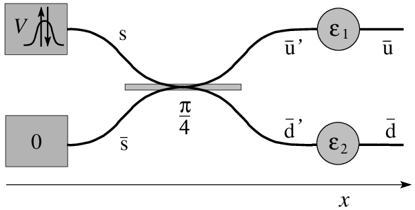
Fundamental quantum phenomena, such as non-locality and entanglement of quantum degrees of freedom, have regained a lot of interest recently, mainly due to their potential usefulness as a computational resource. Mesoscopic physics provides a new platform for the investigation of these phenomena, important issues being the creation, quantification, and verification of non-locality/entanglement. In this paper, we describe an experiment where two electrons with different orbital wave functions are superposed in an interferometer and analyzed in a Bell type experiment involving two-particle correlation measurements, see Fig. 1. The particular feature of this Bell test is the replacement of the four different settings of local detectors in the original setup by four different time-delays in the measured correlators. The main physical property we want to exploit is the indistinguishability of quantum particles, which results in a specific interference between different trajectories. We wish to convey three messages: first, the non-locality in the time-delayed correlations due to indistinguishability manifests itself in the violation of a Bell inequality. Second, the degree of violation is related to the accuracy of the measurement and is reduced, once the local measurement can distinguish between the different orbital wave functions of the particles. The above two items refer to spinless objects (or particles with equal spin). Third, adding the spin degree of freedom, we show how the symmetry relation between spin- and orbital components allows to extract information on spin-entanglement from an orbital measurement.

By now, numerous proposals have been made how to create entangled states in mesoscopic setups, both for orbital- and spin degrees of freedom review. The verification and quantification of entanglement can be carried out using Bell inequality checks cht_00 or state tomography loss_03; buttiker; fazio. The indistinguishability of (spinless) particles producing a two-particle Aharonov-Bohm effect and entanglement has been exploited in a Hanbury-Brown Twiss interferometer SamBut_03; Heiblum_07; here, we offer an alternative implementation which makes use of an electron beam splitter. Using the same setup as discussed here, Burkhard et al.loss_00 have demonstrated how to distinguish between singlet and triplet spin-states by a measurement of zero-frequency cross-correlations. Below, we exploit that the orbital measurement of the Bell parameter preserves the spin-entanglement; this feature allows us to find a lower bound on the concurrence of the spin wave function.
In the following, we consider a setup with two incoming leads, denoted as and , connected to two outgoing leads and through a reflectionless four-terminal beam splitter, see Fig. 1. At time two electrons with normalized orbital wave functions and and common spin state are injected into the leads and . The state, factorizable in orbital and spin parts (with factorized orbital part and general spin part), is conveniently written within a second quantized formalism,
| (1) | |||
here, creates electrons at the position in lead and is the vacuum state with no electrons. After mixing in a four-terminal splitter (with mixing angle ), we will analyze correlations in the system through detection of particles in time (see Fig. 1) or space separated intervals and (see Fig. 3). Our focus then is on the entanglement of the lead indices u and d with respect to bipartitioning of the system between the time or space intervals and .
II Bell test
The particles in the outgoing leads and are subjected to a Bell test expressed through time-resolved current-current correlators in the leads and , (both auto- and crossed- correlators are considered),
| (2) |
where is the total current operator (summed over spin degrees of freedom) in lead at position and time . The time integration is taken over a finite time interval (same for ) with the width accounting for the finite time-resolution of the current measurement, cf. Fig. 1; the limit corresponds to a measurement of the instantaneous current. In the following, we will assume that all correlators are measured at some fixed symmetric position and omit the coordinate variable.
With only two electrons present in the system and for non-overlapping time-intervals , the correlation function is proportional to the joint probability for the detection of two particles during the time intervals and in the leads and , see Ref. Lebedev_05. There are four distinct possibilities to distribute two electrons between the outgoing leads and we can define the properly normalized () probabilities as
| (3) |
Out of these, we define the two-particle Bell inequality in the Clauser-Horne clauser form in the same way as it is done in the usual optics context aspect: we introduce the Bell correlation functions
| (4) |
and obtain the Bell inequality
| (5) |
Here, the polarizations in the optics context are replaced by the lead indices and and the role of the four different polarization settings of the detectors is played by four different time intervals , and , . The violation of this inequality for a particular choice of time intervals shows that non-local correlations are present in the system, i.e., the result of the measurement cannot be simulated by any local-variable theory.
Let us demonstrate that the above Bell inequality indeed can be violated by the incoming state (1) after proper projection. We then have to calculate the four current-current auto- and cross-correlators with and , respectively. This is done within the scattering matrix approach to quantum noise transport: we assume that the Fourier components and of the single-particle wave functions are concentrated near the wave vector , allowing us to linearize the energy–momentum dispersion near . The time evolution of the incoming state (1) then is described by the propagation of the single-particle wave packets and with constant velocity to the right, and , where is a retarded variable. With the scattering matrix of the beam splitter (parametrized by the angle ),
| (6) |
we can express the current operators in the outgoing leads through the electronic scattering states. Averaging the product of current operators in Eq. (2) over the incoming state one arrives at the results
| (7) | |||
| (8) | |||
where describes the overlap between the spin states of the two electrons in the incoming state (1). The two other correlation functions and are obtained by exchanging and in Eqs. (7) and (8). Substituting these expressions for the current correlators into Eq. (2) and integrating over (non-overlapping) time intervals and , one arrives at the Bell correlation function Eq. (4)
| (9) |
where we have introduced the particle densities and averaged over the time intervals and ,
| (10) |
(and similarly for with replaced by ). The overlap between different single particle wave functions reads
| (11) |
In the following, we apply the result (9) first to spinless fermions and plane wave states and and confirm the violation of the Bell inequality in this simple situation. We then proceed with a rederivation of the expression (9) with space-like separated measurement intervals and in order to make the origin of the entanglement more transparent. A formulation in terms of reduced density matrices leading to an expression of the Bell correlator in terms of concurrences completes the discussion.
II.1 Spinless fermions
We first concentrate on spinless particles; this situation can be realized by preparing the two electrons in equal spin-states, with corresponding overlap . To begin with, we choose a plane wave form for the wave packets with different momenta and close to (in order to allow for the linearized spectrum), and . The correlation function takes the form
| (12) |
where is the relative phase shift accumulated by the two waves between the two measurement intervals and is the frequency mismatch between the two plane waves. The phase shift replaces the angle between the two polarizers in the conventional Bell setup. The visibility factor accounts for the width of the time interval,
| (13) |
The other correlation functions involving intervals and are obtained in the same way; their combination into the Bell inequality Eq. (5) produces a maximal violation for the angles and , corresponding to measurement intervals with relative distance , , and , where and is an arbitrary reference time. In this case the Bell inequality Eq. (5) reduces to
| (14) |
For given , the maximal violation is reached for a symmetric beam splitter with , cf. Fig. 2. Furthermore, the maximally allowed degree of violation can be attained only for , corresponding to a short time measurement of the current value with : hence, the maximal violation of the Bell inequality can be obtained for indistinguishable particles, while a time interval with length beyond Heisenberg’s uncertainty bound allows for a distinction between the two particles and the Bell inequality cannot be violated in this classical situation. For the Bell inequality is always satisfied. Within the region , the Bell inequality (14) is always violated for any mixing angle , although to a lesser degree then in the symmetric point .

Let us discuss the physical origin of the violation. The correlator Eq. (2) measured in the Bell test is finite, provided that both electrons are detected within the time windows and ; in this case, it is proportional to the probability . Although, formally, the electrons have different energies and thus are distinguishable in principle, given a small time resolution of the local current measurements one cannot distinguish between the energies and . Under this circumstances the electrons indeed can be considered as indistinguishable particles. Then, according to the rules of quantum mechanics, there are two quantum alternatives contributing to a coincident detection of the electrons in and : either the electrons with energies and are detected in the time windows and , respectively, or vice a versa. These two alternatives contribute to the measurement outcome with different phases: in the first case, the phase factor acquired by the two-particle wave function after the first measurement at due to the propagation of the second particle until is given by , while in the second case this phase assumes the value . The phase difference between the two alternatives leads to quantum interference and a corresponding oscillatory dependence (with frequency ) of the probability as a function of time, with an amplitude proportional to the visibility factor . The precise bound on allowing for a violation of the Bell inequality is given by or , corresponding to a measurement where the Heisenberg uncertainty principle for energy–time variables is violated.
II.2 Space-separated domains
In order to understand better the nature of the entanglement observed in (14), we consider a slightly different experiment, where instead of using time-separated detection intervals, the two observers Alice and Bob are measuring the simultaneous appearance of particles in spatially separated regions and of the setup, see Fig. 3; for particles with a linear dispersion, these two experiments are equivalent since a time delayed measurement with at the point corresponds to a coincident measurement at time with . We first concentrate on plane-wave incoming states, where the present setup with spatially separated detectors provides additional insights. In particular, we will see that it is the projection of the non-entangled incoming state onto the two domains and that defines a bipartition of the system with respect to which the lead index becomes entangled. On the other hand, in order to perform a Bell inequality check, we need a set of local ‘rotations’ of the measurement apparatus: in our setup, the parameters generating a suitable set of local ‘rotations’ are determined by the distance between the measurement domains and and by the mixing angle .
A central element in our discussion below is the interchangeability of mixing and projection onto the domains and , where denotes the one-particle scattering matrix of the beam splitter and the tensor product acts on our two-particle state. This interchangeability is a trivial consequence of these two operations affecting different degrees of freedom, coordinates and and lead indices u and d. In terms of these operators, we can relate the incoming and outgoing states via
| (15) |
Assuming that the projections onto , in the outgoing leads and onto , in the incoming leads (see Fig. 3) are ballistically separated (i.e., the measurement in , involves the appropriate ballistic delay time) we can write
| (16) |
Hence, in our discussion we are free to interchange the two operations of mixing and projection.
Consider then an incoming state (before mixing) with single-particle wave functions and with shifted momenta. The state incident from leads and can be written as a simple Slater determinant,
| (17) |
and thus is non-entangled. The lead index of the electron field operator is conveniently regarded as a pseudo-spin.

To start with, we analyze the coincident detection of two particles within the non-overlapping regions and of the incoming leads, see Fig. 3, and select only those events, where each of the observers (Alice in and Bob in ) finds only one particle. For two particles, this projection can be described by the operator , with the particle number operator counting particles in the region of the incoming leads. Projecting the incoming state (17) one arrives at the state
| (18) | |||
where and are equal to and for and vanishing outside. This projected state is no longer a simple Slater determinant and describes a two-particle state entangled in the lead indices and shared between the regions and of the incoming leads. It is instructive to rewrite the state (18) in a pseudo-spin notation: Assuming for simplicity that the intervals and are reduced to individual points and we have
| (19) |
where and denote states of particles localized in and residing in lead and , respectively; the orbital part of the wave function contributes the phase factors with , where is a momentum mismatch. The projected state (19) is in fact maximally entangled in the lead- or pseudo-spin index with respect to bipartitioning the system between the regions and . In the following, we wish to detect this entanglement in a Bell test.
The implementation of a Bell test relies on the ability to locally change the pseudo-spin basis of the particles. To do so, we transmit the original incoming state Eq. (17) through a beam splitter before measuring the presence of particles in the intervals and , now located in the leads u and d to the right of the mixer, see Fig. 3; the mixing then acts as an equal rotation of the (pseudo-spin) basis for both particles. However, such a global rotation of the original basis alone is not sufficient to perform the Bell test, as locally distinct rotations are required as well; the latter are implemented through different choices in the separation between the regions and . Exploiting the interchangeability of projection and mixing, cf. Eqs. (15) and (16), we see that this change in distance results in a relative rotation with the angle around the original -polarization axis of the pseudo spins, see Eq. (19). Writing the outgoing state (16) in pseudo-spin notation, we obtain the expression
| (20) |
This projected state describes two spatially separated localized particles with entangled pseudo spin indices. Choosing different space separations between the regions and allows one to change the phase and mixing by generates a second rotation parametrized by the angle . Calculating the joint probabilities for the four settings we find the Bell correlation functions as given by (9) and choosing appropriate angles and one finds the Bell inequalities violated.
II.3 Density matrix formulation
In a last step, we reformulate our analysis in terms of density matrices and express the Bell inequality in terms of concurrences of density matrices reduced after projection to the intervals and . We rewrite the projected state (18) incident from leads and in pseudo spin representation, , where
| (21) |
The joint measurement of the pseudo-spin index in the regions and is described by the coordinate-reduced two-particle density operator
We introduce the two-particle pseudo-spin basis , where the first (second) arrow refers to the particle localized in (); the normalized density matrix then assumes the form
| (22) |
where , and with . Although initially the two particles have been in a pure state, the reduced density matrix (22) corresponds to a mixed state with . The calculation of the entanglement in the mixed two-particle state Eq. (22) corresponds to finding the concurrence of a two-qubit problem, and thus can be calculated following the scheme introduced by Wootters wootters, where are the eigenvalues of the matrix with , is a Pauli matrix, and denotes the tensor product. The result of this calculation provides us with the expression
| (23) |
This quantity is indeed restricted to the interval , as follows from the Cauchy-Schwartz inequality and the inequality , . The state described by Eq. (22) is trivial (i.e., not entangled or classical) only for zero overlap and/or . Physically, the vanishing of the overlap between the wave functions and in either of the two regions and implies, that these orbital states are perfectly distinguishable via a local measurement. In this situation the corresponding density matrix can be written in a convex form , with probabilities and , and thus is separable. On the other hand, for one cannot perfectly distinguish between the different orbital states via local measurements, resulting in an interference between the different terms of the anti-symmetric wave function Eq. (21), a non-separable density matrix, and a finite concurrence.
Next, we analyze the reduced density matrix in the outgoing leads, i.e., in the new basis . Exploiting the possibility of exchanging real space projection and mixing, we can simply rotate the projected density matrix according to
| (24) |
The diagonal elements of the density matrix directly provide the detection probabilities , which then can be used in the calculation of the Bell correlation function , Eq. (4),
| (25) |
where the angle is given by the overlap integrals, ; combining Eqs. (23) and (25) we immediately recover the original expression (9). Choosing four different intervals , , , and (note that the selection of these intervals is non-trivial in the general situation discussed here, as now involves overlap integrals), we can set up the Bell inequality (5) and find the result expressed in terms of concurrences ,
| (26) | |||
Choosing plane waves for and , the concurrences take the value and the Bell inequality reduces to the simpler form found earlier, see Eq. (14); for the general case, the degree of violation depends separately on the shapes and of the orbital wave functions in each region , , , and via the corresponding concurrences.
II.4 Particles with spin
So far, we have considered only spinless particles or, more exactly, two electrons in a spin-triplet state with the same spin polarization of the electrons, and . Since all spin-dependence of the Bell inequality is encoded in the overlap of the spin wave-functions, see Eq. (9), one concludes that the above results are valid as well for the third maximally entangled triplet state, with . On the other hand, the character of violation is modified for the spin-singlet state with . Choosing a set of optimal time intervals , , , and , the resulting Bell inequality takes the form
| (27) |
The main difference to the previous result for spin-triplet states is that this inequality can be violated only for a sufficiently large visibility factor and a beam splitter with a mixing angle sufficiently close to optimal, , where the critical angle is given by , cf. Fig. 2. This result allows one to distinguish between triplet and singlet incoming states by measuring a Bell inequality involving only orbital degrees of freedom, see also Ref. loss_00.
Moreover, assuming that the incident electrons have opposite spin polarization, i.e., their spin state can be written as a superposition , the degree of violation of the orbital Bell inequality gives a lower bound on the value of the concurrence in the spin part of the wave function. Indeed, in this case and the maximal violation of the orbital Bell inequality for and symmetric scattering is given by . At the same time, the concurrence , with equality established for real and (note that gives the degree of (useful) spin entanglement in the outgoing leads u and d). Hence, measuring the entanglement of the orbital part of the wave function (which leaves the spin component untouched), provides a (lower) estimate of the degree of spin entanglement of the incoming state. If the spin wave function of the incoming electrons factorizes, , the orbital Bell inequality never can be violated since in this situation the electrons are distinguishable and thus the detection of an electron with given spin in one of the outgoing leads always allows to determine its origin.
III Spin-singlet/triplet sources
Finally, we discuss the potential experimental realization of the proposed Bell test. The source of spin-entangled incoming particles can be realized with the help of a beam splitter, followed by leads with dots serving as energy filters defined through resonance levels at energies and , see Fig. 4. We assume that both dots reside in the strong Coulomb blockade regime; applying a single-electron voltage pulse to the source lead , two electrons in a singlet state are detached from the Fermi see lesovik; levitov. There is only one scattering process, involving trajectories where the electrons tunnel through different quantum dots, for which the two electrons reach the second beam splitter. The incoming state in the leads and then is of a spin-singlet type with different energies and as defined through the dot resonances. All other scattering processes with only one or no electrons propagating towards the second beam splitter are irrelevant as they do not contribute to the correlation measurement.
A spin entangled triplet state can be generated with the help of spin-polarized reservoirs with polarizations and attached to the leads and , respectively. Applying a single-electron voltage-pulse to each reservoir, two electrons with opposite spins are injected into the leads and , see Fig. 4. The state incident on the symmetric beam splitter emerges with a component
| (28) | |||||
describing electrons scattered into different leads and ; it is this component which can propagate through the subsequent energy filter and contribute to the current correlators. The propagation of this component through the quantum dots results in an entangled spin-triplet state of the form given by Eq. (1) with and .
Above, we have considered an idealized situation where only two electrons are present in the system, while in a realistic situation one deals with electronic reservoirs at finite temperature. The associated equilibrium fluctuations then generate noise signals which are of the same order as the correlations associated with the injection of the two electrons. We note, however, that the corresponding equilibrium current correlators assume significant values only for instantaneous or ballistically retarded variables, i.e., at times and in the same leads and in opposite leads (here, denotes the distance between the position of measurement and the reflecting dots). The Bell test involves correlations at time differences of the order of and a proper choice of the frequency mismatch always allows one to render the contribution from equilibrium fluctuations negligible. Another restriction on is due to dephasing and electron-electron interactions; we then have to assume that the characteristic times associated with these processes are larger then .
IV Conclusion
We have discussed how to make use of quantum indistinguishability as a resource to generate non-classical correlations: the indistinguishability of particles enforces proper symmetrization of their wave function and results in non-factorizable states. We have demonstrated how to generate such states with the help of quantum dots residing in the Coulomb blockade regime and have determined their degree of entanglement as measured in a Bell inequality test based on auto- and cross-current correlators. In a real experiment, the latter are measured over a finite time or space domain. As a result, we obtain an interesting interplay between the measurement accuracy (time or space resolution) and the degree of non-locality as measured in the Bell inequality test: the more information is gained that locally distinguishes between the particles, the smaller is the degree of violation. Once the uncertainty principle allows for the identification of the particle, the Bell inequality cannot be violated any longer. This feature can be exploited in the design of experiments testing the above predictions: choosing a small energy difference allows for a slow measurement with a less stringent time resolution, while the violation of the Bell test remains observable. On the other hand, the energy difference has to be chosen sufficiently large in order to avoid the influence of decoherence or interactions.
The above setup for spinless particles provides an alternative for the observation of the two-particle interference as proposed by Samuelsson et al. SamBut_03 and recently observed by Neder et al. Heiblum_07; here, the role of the magnetic flux penetrating the Hanbury-Brown Twiss interferometer is replaced by the time-delay of subsequent measurements in the correlator. Adding the spin degree of freedom, we are confronted with two distict situations: if the spin degree of freedom allows to distinguish between the particles (this is the case for the spin-state ) the Bell inequality is never violated. On the other hand, entangled spin states in the singlet or triplet sector (these are the states and ) can generate maximal violation of the Bell inequality; finally, the superposition of these states reduces the spin-entanglement and the degree of violation in the orbital Bell inequality gives a lower bound on the spin-concurrence, with an ideal measurement providing the best bound.
We thank Gordey Lesovik for discussions and acknowledge the financial support from the Swiss National Foundation, the RFBR grant No. 06-02-17086-a and the Programm “Quantum Macrophysics” of RAS.
References
- (1) C. W. J. Beenakker, in Quantum Computers, Algorithms and Chaos, Proceedings of the Int. School of Physics “Enrico Fermi”, Varenna 2005, Vol. 162 (IOS Press, Amsterdam, 2006); arXiv:cond-mat/0508488.
- (2) N. M. Chtchelkatchev, G. Blatter, G. B. Lesovik, and Th. Martin, Phys. Rev. B 66, 161320(R) (2002).
- (3) G. Burkard, and D. Loss, Phys. Rev. Lett. 91, 087903 (2003).
- (4) P. Samuelsson and M. Büttiker, Phys. Rev. B 73, 041305 (2006).
- (5) V. Giovannetti, D. Frustaglia, F. Taddei, and R. Fazio, Phys. Rev. B 74, 115315 (2006); V. Giovannetti, D. Frustaglia, F. Taddei, and R. Fazio, Phys. Rev. B 75, 241305(R) (2007).
- (6) P. Samuelsson, E. V. Sukhorukov, and M. Büttiker, Phys. Rev. Lett. 92, 026805 (2004).
- (7) I. Neder, M. Heiblum, D. Mahalu, and V. Umansky, Phys. Rev. Lett. 98, 036803 (2007) and I. Neder, N. Ofek, Y. Chung, M. Heiblum, D. Mahalu, and V. Umansky, Nature 448, 333 (2007).
- (8) G. Burkard, D. Loss, and E. V. Sukhorukov, Phys. Rev. B 61, R16303 (2000).
- (9) A.V. Lebedev, G.B. Lesovik, and G. Blatter, Phys. Rev. B 71, 045306/1-9 (2005); note that with only two incident electrons there is no restriction on the accumulation time, see Sec. III B.
- (10) J.F. Clauser and M.A. Horne, Phys. Rev. D 10, 526 (1974).
- (11) A. Aspect, P. Grangier, and G. Roger, Phys. Rev. Lett. 49, 91 (1982).
- (12) G. B. Lesovik, JETP Lett. 49, 592 (1989); M. Büttiker, Phys. Rev. Lett. 65 2901 (1990); Ya. M. Blanter and M. Büttiker, Phys. Rep. 336, 1 (2000).
- (13) W. K. Wootters, Phys. Rev. Lett. 80, 2245 (1998).
- (14) L. S. Levitov, H. W. Lee, and G. B. Lesovik, J. Math. Phys. 37, 4845 (1996).
- (15) J. Keeling, I. Klich, and L. S. Levitov, Phys. Rev. Lett. 97, 116403 (2006).