We begin with recalling some general facts about intersecting branes in IIB string theory. In this theory supersymmetry transformations are parameterized by two Majorana–Weyl spinors which have the same chirality, and it is convenient to combine them into a 32–component real object $\epsilon$ which satisfies a chirality projection:

$\displaystyle\epsilon=\left(\begin{array}[]{c}\epsilon_{1}\\ \epsilon_{2}\end{array}\right),\quad{\bf 1}_{2}\otimes\Gamma_{11}\epsilon=-\epsilon:\qquad\Gamma_{11}\epsilon_{1,2}=-\epsilon_{1,2}.$

Ten–dimensional flat space preserves $32$ supersymmetries corresponding to arbitrary constant values of $\epsilon_{1}$ and $\epsilon_{2}$ (modulo the chiral projection). By adding a brane to $R^{9,1}$ one breaks half of the supersymmetries and the appropriate projections are [20] (see also [17] for a review):

	$\displaystyle{\rm F1}:$	$\displaystyle\quad\Gamma=\sigma_{3}\otimes\Gamma_{(2)},\quad$	$\displaystyle\Gamma\epsilon=\epsilon,$
	$\displaystyle{\rm NS5}:$	$\displaystyle\quad\Gamma=\sigma_{3}\otimes\Gamma_{(6)},\quad$	$\displaystyle\Gamma\epsilon=\epsilon,$		(2.4)
	$\displaystyle{\rm D}(2p-1):$	$\displaystyle\quad\Gamma=i\sigma^{p}_{3}\sigma_{2}\otimes\Gamma_{(2p)},\quad$	$\displaystyle\Gamma\epsilon=\epsilon.$

Here $\Gamma_{(2p)}$ is a product of gamma matrices with indices pointing along the worldvolume of the brane. Each of the branes appearing in (2.1) preserves $16$ real supercharges and there are two other interesting objects which have the same amount of SUSY --- a plane wave and a KK monopole³³ 3 To unify the description of KK monopoles in ten and eleven dimensions, we characterize the monopole by four nontrivial coordinates rather than by $5+1$ (or $6+1$) worldvolume directions.:

	$\displaystyle{\rm P}:$	$\displaystyle\quad\Gamma={\bf 1}_{2}\otimes\Gamma_{(2)},\quad$	$\displaystyle\Gamma\epsilon=\epsilon,$
	$\displaystyle{\rm KK}:$	$\displaystyle\quad\Gamma={\bf 1}_{2}\otimes\Gamma_{(4)},\quad$	$\displaystyle\Gamma\epsilon=\epsilon.$		(2.5)

These configurations have a pure geometric nature and they do not involve fluxes.

Once the building blocks preserving half of the supersymmetries are specified, one can start combining them to produce configurations with lower SUSY. Such supersymmetric intersections are only possible if the projectors for the ingredients commute with each other. The main example studied in this paper involves fundamental strings ending on a D3 brane:

$\displaystyle\begin{array}[]{c|ccccccccc}&1&2&3&4&5&6&7&8&9\\ D3&\bullet&\bullet&\bullet&&&&&&\\ F1&&&&\bullet&&&&&\\ \end{array}$

Looking at spinors preserved by each object:

	$\displaystyle D3:$		$\displaystyle i\sigma_{2}\otimes\Gamma_{0123}\epsilon_{3}=\epsilon_{3},$
	$\displaystyle F1:$		$\displaystyle{\bf 1}_{2}\otimes\Gamma_{04}\epsilon_{1}=\epsilon_{1},$

we observe that two projectors can be diagonalized simultaneously and the entire configuration preserves $8$ supercharges. In fact, one more object can be added to this system without breaking additional supersymmetry:

$\displaystyle D5_{56789}:$

$\displaystyle\sigma_{1}\otimes\Gamma_{056789}\epsilon_{5}=\epsilon_{5},$

so it is useful to look at the following configuration:

$\displaystyle\begin{array}[]{c|ccccccccc}&1&2&3&4&5&6&7&8&9\\ D3&\bullet&\bullet&\bullet&&&&&&\\ D5&&&&&\bullet&\bullet&\bullet&\bullet&\bullet\\ F1&&&&\bullet&&&&&\\ \end{array}$

Performing a similar analysis, one can classify all brane intersections preserving $8$ supercharges⁴⁴ 4 We omit the configurations which can be found by an application of S duality (e.g. $(D3_{123},\mbox{NS5}_{56789},D1_{4})$).:

	$\displaystyle(D3_{123},D5_{56789},F1_{4}),~(D3_{123},D3_{145},KK_{2345}),~(D3_{123},D5_{12456},\mbox{NS5}_{12789}),$
	$\displaystyle\quad\qquad(D5_{12345},D7_{1234678},\mbox{NS5}_{12349}),\quad(D7_{1234567},F1_{8},D1_{9})$		(2.15)
	$\displaystyle\qquad(D5_{12345},D5_{16789},P_{1}),\quad(D3_{123},D7_{1456789},P_{1}),\quad(D1_{1},P_{1})$
	$\displaystyle\quad\qquad(D5_{12345},D1_{1},KK_{2345}),\quad(D3_{123},D7_{1234567},KK_{4567}).$

To construct the geometries corresponding to intersections appearing in the last two lines, one needs to superpose harmonic functions and some of the resulting solutions are well–known [21]. The geometries describing localized intersections presented in the first two lines has not been written before, and our main goal is to find the appropriate metrics. It turns out that once the description of (2.1) is known, the other configurations appearing in (2.1) can be recovered by application of various dualities, so most of our discussion will be concentrated on (2.1) and we will come back to other configurations in section 4.7.

Finally let us comment on branes in M theory. One still has geometric objects characterized by projections (2.1), and in addition there are M2 and M5 branes which preserve the following pieces of the 32–component real spinor $\epsilon$ [22, 23, 24, 25]:

	$\displaystyle{\rm M2}:$	$\displaystyle\quad\Gamma=\Gamma_{(3)},\quad$	$\displaystyle\Gamma\epsilon=\epsilon,$
	$\displaystyle{\rm M5}:$	$\displaystyle\quad\Gamma=\Gamma_{(6)},\quad$	$\displaystyle\Gamma\epsilon=\epsilon.$

The intersections preserving $8$ supersymmetries can be classified in this case as well:

	$\displaystyle(M5_{12345},M5_{1789(10)},M2_{16}),~(M5_{12345},KK_{1234},P_{5}),~(KK_{1234},M2_{12},M2_{34}),$		(2.16)
	$\displaystyle(M5_{12345},M5_{12367},KK_{4567}),~(KK_{1234},KK_{5678},M2_{9(10)})$
	$\displaystyle(KK_{1234},KK_{1256},KK_{3456}),~(M5_{12345},KK_{6789}),~(M2_{12},P_{1}).$

and we will discuss the corresponding geometries in section 5.

However before we start constructing supergravity solutions, it is useful to perform a brane probe analysis. We will see that some intersections are described by curved branes with fluxes on their worldvolumes and we will find the shapes of such branes. This analysis will be presented both in type IIB string theory (using D3–D5–F1 system as an example) and in M theory (where we discuss M5–M5–M2 intersection).

We begin by recalling the solution found by Callan and Maldacena [15]. The basic idea of that work can be summarized in the following way. Suppose one wants to describe a fundamental string ending on Dp brane (as depicted in figure 1a). This configuration is expected to preserve eight real supercharges. An observer living on the D brane sees a pointlike charge, so an electric field should be excited on the worldvolume of the brane. This modifies the shape of the D brane, and the correct physical picture is given by figure 1b rather than 1a: the fundamental string is replaced by a curved brane with flux. Let us review this construction in more detail.

The starting point for the analysis of [15] was a special embedding of Dp brane into the ten dimensional space, so that the brane was stretched along the directions $X^{0},\dots X^{p}$, while it was also allowed to have a nontrivial profile in one of the transverse coordinate $X\equiv X^{p+1}$. To have interesting dynamics, one also allows for a non–vanishing electric field on the worldvolume of the brane. In the static gauge ($X^{0}=\xi^{0}$,…,$X^{p}=\xi^{p}$) the DBI action for Dp brane becomes

	$\displaystyle S_{Dp}$	$\displaystyle=$	$\displaystyle-T_{p}\int d^{p+1}\xi\sqrt{-\mbox{det}(G+2\pi\alpha^{\prime}F)}$		(2.17)
		$\displaystyle=$	$\displaystyle-T_{p}\int d^{p+1}\xi\sqrt{(1-E^{2})(1+(\nabla X)^{2})+({\bf E}\nabla X)^{2}}.$

Here electric field is defined as $E_{i}=2\pi\alpha^{\prime}F_{i0}$. Since we are looking for a static solution, it is convenient to choose a gauge ${\bf E}=\nabla A$, this leads to the equations of motion for two scalars $X,A$:

	$\displaystyle\nabla_{i}\left[\frac{(1-(\nabla A)^{2})\nabla_{i}X+(\nabla A\nabla X)\nabla_{i}A}{\sqrt{(1-(\nabla A)^{2})(1+(\nabla X)^{2})+(\nabla A\nabla X)^{2}}}\right]=0,$
	$\displaystyle\nabla_{i}\left[\frac{(1+(\nabla X)^{2})\nabla_{i}A+(\nabla A\nabla X)\nabla_{i}X}{\sqrt{(1-(\nabla A)^{2})(1+(\nabla X)^{2})+(\nabla A\nabla X)^{2}}}\right]=0.$

In [15] it was pointed out that these equations linearize it we take $A=X$. Moreover, in this case the solution saturates the BPS bound since it has a very simple energy density:

$\displaystyle{\cal E}={\bf E}\frac{\delta S_{Dp}}{\delta{\bf E}}-{\cal L}=T_{p}\left(1+(\nabla X)^{2}\right).$

(2.18)

To summarize, the construction of [15] gives a family of 1/4–BPS configurations which are parameterized by one harmonic function $X$:

$\displaystyle\nabla^{2}X=0,\quad F_{0i}=\frac{1}{2\pi\alpha^{\prime}}\nabla_{i}X,$

(2.19)

and this function gives a location of the brane. Let us discuss the symmetries of the problem. Since the brane is curved in one of the transverse directions, the rotations around the brane are broken to $SO(8-p)$ and for a generic profile of $X$ this is the only non--abelian symmetry of the configuration⁵⁵ 5 Since the system is static, it is also invariant under time translations.. However for special functions $X$ there might be additional symmetry coming from the worldvolume of the brane. For example, figure 1a suggests an $SO(p)$ rotational symmetry around the string, so it is natural to consider a single spike which is invariant under such rotations. Thus we see that the maximally symmetric spike has an $SO(8-p)\times SO(p)\times U(1)$ symmetry, in particular both D3 and D5 branes are invariant under $SO(5)\times SO(3)\times U(1)$. This symmetry will be further explored in section 3.

Let us now make a comment about emergence of fundamental strings. Due to nontrivial value of the electric field, the action (2.17) sources a bulk Kalb–Ramond field even in the linear order [26]. The simplest way to find the relevant coupling is to make a substitution $2\pi\alpha^{\prime}F\rightarrow 2\pi\alpha^{\prime}F-P[B]$ in (2.17) and compute the first correction:

	$\displaystyle\delta S_{p}$	$\displaystyle=$	$\displaystyle-\int d^{p+1}\xi\frac{\delta S_{p}}{\delta(2\pi\alpha^{\prime}F_{\mu\nu})}P[B]_{\mu\nu}=T_{p}\int d^{p+1}\xi P[B]_{ti}\nabla_{i}X$		(2.20)
		$\displaystyle=$	$\displaystyle T_{p}\int d^{p+1}\xi(B_{ti}+(\nabla_{i}X)B_{t(p+1)})\nabla_{i}X.$

Here $P[B]$ is a pullback of the B field to the worldvolume of the brane.

It is interesting to look at a single spherically symmetric spike which has $X=Qr^{-(p-2)}$, for this configuration the coupling to the Kalb–Ramond field becomes:

$\displaystyle\delta S_{p}$

$\displaystyle=$

$\displaystyle T_{p}\Omega_{p-1}\int dX\left[r^{p-1}B_{tr}-Q(p-2)B_{t(p+1)}\right].$

(2.21)

As expected, in the region where the spike becomes thin (i.e. close to the origin in $r$ coordinate) this term sources strings stretching in $(t,X^{p+1})$ directions with a density which is uniform in $X^{p+1}=X$.

In the previous subsection we recalled the description of spikes on Dp branes assuming that these branes are placed in the flat space. In particular we observed that a single spike attached to a D3 brane has the same $SO(5)\times SO(3)\times U(1)$ symmetry as a spike attached to D5. This leads to a natural proposal to consider these two types of branes together. In the probe approximation superposition of branes leads to addition of their DBI actions, so the analysis of the previous subsection goes through. However branes with different orientations preserve different supersymmetries, so in general a combination of branes would break SUSY completely. Of course, in the exceptional cases some SUSY is still preserved and as we reviewed in section 2.1, the combination of D3, D5 branes and fundamental strings preserves eight supercharges. Moreover, by building configuration (2.1) from one stack of D3 branes and one stack of D5s, we can also preserve $SO(5)\times SO(3)\times U(1)$ bosonic symmetry. In a more general case when we have several D3 and D5 branes at various positions, the $SO(5)\times SO(3)$ symmetry would be broken, but eight supersymmetries will still be preserved as long as the orientations of the branes are the same as in (2.1).

To probe this picture one can consider the following setup. Suppose one starts with large number of D3 branes without strings attached to them. These branes would lead to the modification on the geometry, and the resulting metric is well–known [2]. Then to describe an additional D3 brane with string ending on it, one needs to solve the equations of motion coming from the DBI action on curved background. It would be interesting to find a profile of the spike in this case. One can also look at the D5 brane on D3 background and solve equations in this case as well. The D branes in the geometry produced by multiple D5’s can be analyzed in the same way. While these exercises are very straightforward, it seems useful to outline them here since we will need to compare the results with the outcome of computations in supergravity.

D3 spike in the geometry of D3. This case has been previously analyzed in [27], so we will be very brief. The background geometry is given by the metric of $N$ coincident D3 branes⁶⁶ 6 In this section we use the string conventions which has a different normalization of $F_{5}$ compared to standard supergravity notation. We discuss this difference in more detail in Appendix A (see also [30]). [2]:

	$\displaystyle ds^{2}$	$\displaystyle=$	$\displaystyle H^{-1/2}ds_{3,1}^{2}+H^{1/2}(dz^{2}+d{\bf y}_{5}^{2}),$
	$\displaystyle F_{5}$	$\displaystyle=$	$\displaystyle d\left[H^{-1}d^{4}x\right]-^{*}_{6}dH,\quad H=1+\frac{Q}{(z^{2}+{\bf y}^{2})^{2}},\quad Q=4\pi gN\alpha^{\prime}.$		(2.22)

One can study dynamics of a probe D3 brane assuming that its worldvolume is described by a profile $r=0$, $z=X(x_{1},x_{2},x_{3})$. In the static gauge ($\xi_{0}=x_{0}$, …, $\xi_{3}=x_{3}$) the induced metric and the pullback of the RR potentials are

$\displaystyle G_{ab}=H^{-1/2}\eta_{ab}+H^{1/2}\partial_{a}X\partial_{b}X,\quad C_{abcd}=H^{-1}\epsilon_{abcd}$

(2.23)

and the action governing the dynamics of the probe brane becomes⁷⁷ 7 Here we again defined $E_{i}=2\pi\alpha^{\prime}F_{i0}=\nabla_{i}A$.:

	$\displaystyle S_{D3}$	$\displaystyle=$	$\displaystyle-T_{3}\int d^{4}\xi\sqrt{-\mbox{det}(G+2\pi\alpha^{\prime}F)}+\frac{T_{3}}{4!}\int C_{abcd}d\xi^{abcd}$		(2.24)
		$\displaystyle=$	$\displaystyle-T_{3}\int d^{4}\xi H^{-1}\sqrt{(1-HE^{2})(1+H(\nabla X)^{2})+H^{2}({\bf E}\nabla X)^{2}}$
			$\displaystyle+T_{3}\int d^{4}\xi H^{-1}.$

One can see that equations of motion for $A$ and $X$ are satisfied if the relations (2.19) are imposed⁸⁸ 8 Notice that the Chern–Simons term is the action is crucial for enforcing a condition $\frac{\partial{\cal L}}{\partial X}=0$.. We conclude that even in the background produced by other D3s, the spike of D3 brane should still follow the harmonic profile in $\xi_{1}$, …, $\xi_{3}$.

D5 spike in the geometry of D3. Next we put a D5 brane in the background written above⁹⁹ 9 Such brane is relevant for the description of baryons in AdS/CFT [28] and its DBI dynamics has been discussed in [29]. Unfortunately, the coordinate system used in [29] is not very convenient for comparison with gravity solutions, so we need an alternative derivation presented below.. Using the static gauge $\xi_{0}=x_{0}$, …, $\xi_{5}=y_{5}$ and writing $z=Y(y_{1},\dots,y_{5})$, we find the induced metric $G_{AB}$ and the DBI action:

	$\displaystyle G_{00}=-H^{-1/2},\quad G_{ab}=H^{1/2}\left[\delta_{ab}+\partial_{a}X\partial_{b}X\right],\quad E_{a}=\nabla_{a}A,$
	$\displaystyle S^{DBI}_{D5}=-T_{5}\int d^{6}\xi H\sqrt{(1-E^{2})(1+(\nabla X)^{2})+({\bf E}\nabla X)^{2}}.$		(2.25)

While in the absence of the electric field there is no direct coupling between D5 brane and four–form potential, in the present case we do have a nontrivial contribution to the Chern–Simons term:

$\displaystyle S^{CS}_{D5}$

$\displaystyle=$

$\displaystyle T_{5}\int_{D5}2\pi\alpha^{\prime}F\wedge P[{\tilde{C}}_{4}]=-T_{5}\int d\xi^{0}\int_{\mbox{vol}}dA\wedge P[{\tilde{C}}_{4}].$

(2.26)

Here ${\tilde{C}}_{4}$ is defined by the relation

$\displaystyle d{\tilde{C}}_{4}=^{*}_{6}dH=-\frac{4Q}{(z^{2}+{\bf y}^{2})^{3}}~^{*}_{6}\left[zdz+{\bf y}d{\bf y}\right].$

In particular if we choose a convenient gauge where

$\displaystyle{\tilde{C}}_{4}=4Qy_{a}\frac{\epsilon_{abcde}}{4!}dy_{bcde}\int_{0}^{z}\frac{dw}{(w^{2}+{\bf y}^{2})^{3}},$

then the pullback is especially simple. Plugging this expression in (2.26), we can simplify the Chern–Simons coupling:

$\displaystyle S^{CS}_{D5}=-T_{5}\int d\xi^{0}\int_{\mbox{vol}}d\left[A{\tilde{C}}_{4}\right]+4QT_{5}\int d^{6}\xi A\partial_{a}\left[\int^{X}\frac{y_{a}dw}{(w^{2}+{\bf y}^{2})^{3}}\right].$

Using the relation

$\displaystyle 4\partial_{a}\left[\int^{X}\frac{y_{a}dw}{(w^{2}+{\bf y}^{2})^{3}}\right]=-\partial_{a}\partial_{a}\int^{X}\frac{dw}{(w^{2}+{\bf y}^{2})^{2}}+\partial_{a}\frac{\partial_{a}X}{(z^{2}+{\bf y}^{2})^{2}}$

and dropping total derivatives from the Chern--Simons action¹⁰¹⁰ 10 We are looking for configurations where gauge potential $A$ decays sufficiently fast as we go to infinity on the D5 brane, so the boundary terms do not contribute., we arrive at the final expression:

$\displaystyle S^{CS}_{D5}=-T_{5}\int d^{6}\xi\nabla^{2}A\int_{0}^{X}dw(H-1)|_{z=w}-T_{5}\int d^{6}\xi(H-1)|_{z=X}\partial_{a}A\partial_{a}X.$

(2.27)

To summarize, the action for the D5 brane is given by a sum of (2.25) and (2.27). Writing equations of motion for $X$ and $A$ and setting $A=X$ in the result, we find

	$\displaystyle-\partial_{X}H+\nabla(H\nabla X)-(H-1)\nabla^{2}X-\partial_{X}H(\nabla X)^{2}+\nabla((H-1)\nabla X)=0,$
	$\displaystyle-\nabla(H\nabla X)-\nabla^{2}\int_{0}^{X}dw(H-1)_{w}+\nabla((H-1)\nabla X)=0.$

To simplify the second equation, we rewrite the term containing the integral in a more transparent form¹¹¹¹ 11 Here we defined ${\tilde{\nabla}}_{i}H$ as a derivative taken at fixed value of $z$. Its relation to a total derivative is given by ${\tilde{\nabla}}_{i}H=\nabla_{i}H-\partial_{X}H\nabla_{i}X$. We also used the fact that $H$ is harmonic.

	$\displaystyle\nabla^{2}\int_{0}^{X}dw(H-1)_{w}$	$\displaystyle=$	$\displaystyle\nabla((H-1)\nabla X)+\nabla X{\tilde{\nabla}}(H-1)+\int_{0}^{X}dw{\tilde{\nabla}}^{2}(H-1)|_{z=w}$
		$\displaystyle=$	$\displaystyle(H-1)\nabla^{2}X+2\nabla(H-1)\nabla X-((\nabla X)^{2}+1)\partial_{X}H.$

Using this expression, one concludes that equations for $X$ and $A$ collapse to the same relation:

$\displaystyle-(1+(\nabla X)^{2})\partial_{X}H+H\nabla^{2}X+2\nabla H\nabla X=0.$

(2.28)

Even though this relation looks more complicated than the Laplace equation (2.19), in section 4.2 we will see that (2.28) has a very simple interpretation once it is rewritten in different coordinates.

D3 spike in the geometry of D5. Let us now consider probes in the geometry produced by $N$ coincident D5 branes¹²¹² 12 In this paper most of the metrics are written in the Einstein frame. However since the DBI action is usually written in terms of the string metric, we use this frame in (2.29).:

	$\displaystyle ds_{S}^{2}=H^{-1/2}(-dt^{2}+d{\bf y}_{5}^{2})+H^{1/2}(dz^{2}+d{\bf x}_{3}^{2}),$		(2.29)
	$\displaystyle e^{2\Phi}=H^{-1},\quad F_{3}=^{*}_{10}(dH^{-1}\wedge dt\wedge d^{5}y)=^{*}_{3}dH,\quad H=1+\frac{Q}{(z^{2}+{\bf x}^{2})}.$

We begin with putting a D3 brane on this background. As one goes to infinity, the effect of D5 branes become negligible, and in this region we expect the D3 brane to stretch along $t$ and $x_{1},x_{2},x_{3}$. This suggests a natural static gauge which can be imposed everywhere: $\xi^{0}=t$, $\xi_{i}=x_{i}$. The action describing D3 brane contains the DBI piece, and, in the presence of the electric field, there is also a Chern–Simons coupling with two–form potential. We analyze these two terms separately starting with DBI contribution:

	$\displaystyle S^{DBI}_{D3}$	$\displaystyle=$	$\displaystyle-T_{3}\int d^{4}\xi e^{-\Phi}\sqrt{-\mbox{det}(G+2\pi\alpha^{\prime}F)}$		(2.30)
		$\displaystyle=$	$\displaystyle-T_{3}\int d^{4}\xi H\sqrt{(1-E^{2})(1+(\nabla X)^{2})+({\bf E}\nabla X)^{2}}.$

The evaluation of the Chern–Simons term follows the same steps as the derivation of (2.27), so we will be brief here. If one chooses a convenient gauge for $C_{2}$:

$\displaystyle C_{2}=2Qx_{a}\frac{\epsilon_{abc}}{2}dx_{bc}\int_{0}^{z}\frac{dw}{(w^{2}+{\bf x}^{2})^{2}},$

(2.31)

then up to total derivatives, the Chern-Simons action becomes:

	$\displaystyle S^{CS}_{D3}$	$\displaystyle=$	$\displaystyle T_{3}\int_{D}32\pi\alpha^{\prime}\wedge P[C_{2}]=2QT_{3}\int d^{4}\xi A\partial_{a}\left[\int_{0}^{X}\frac{x_{a}dw}{(w^{2}+{\bf x}^{2})^{2}}\right]$		(2.32)
		$\displaystyle=$	$\displaystyle-T_{3}\int d^{4}\xi\left\{\nabla^{2}A\int_{0}^{X}dw(H-1)+(H-1)\partial_{a}A\partial_{a}X\right\}.$

We observe that the action for D3 brane superficially looks the same as the sum of (2.25) and (2.27), although the harmonic functions and the number of independent variables appearing in these two cases are different. In spite of this differences, one can see that the same manipulations that led to the (2.28) can be repeated here, and we conclude that for configurations with $A=X$ there is only one independent equation of motion:

$\displaystyle-(1+(\nabla X)^{2})\partial_{X}H+H\nabla^{2}X+2\nabla H\nabla X=0.$

(2.33)

D5 branes in D5 background. Finally we analyze the D5 brane in the geometry (2.29). To do this it is convenient to describe the Ramond–Ramond field in terms of the dual six–form potential:

$\displaystyle C_{6}=H^{-1}dt\wedge d^{5}y.$

(2.34)

Then the action for D5 brane becomes:

	$\displaystyle S_{D5}$	$\displaystyle=$	$\displaystyle-T_{5}\int d^{5}\xi H^{-1}\sqrt{(1-HE^{2})(1+H(\nabla X)^{2})+H^{2}({\bf E}\nabla X)^{2}}$		(2.35)
			$\displaystyle+T_{5}\int d^{4}\xi H^{-1}.$

Equations of motion are satisfied by ${\bf E}=\nabla X$ as long as $X$ is a harmonic function.

In the last two subsections we discussed various configurations of branes with fluxes in type IIB string theory. A similar analysis can be performed in M theory as well and we will outline it here.

M theory has two fundamental objects: M2 and M5 branes. In string theory we looked at fundamental strings ending on D brane, and the closest analog of this configuration in eleven dimensions is a set of membranes ending on M5 brane. To preserve supersymmetry, the branes should intersect on a line, and the third object can be added without breaking additional supersymmetry:

$\displaystyle\begin{array}[]{c|cccccccccc}&1&2&3&4&5&6&7&8&9&10\\ M5&\bullet&\bullet&\bullet&\bullet&\bullet&&&&&\\ M2&&&&&\bullet&\bullet&&&&\\ M5^{\prime}&&&&&\bullet&&\bullet&\bullet&\bullet&\bullet\\ \end{array}$

Notice that one can arrive at configuration (2.4) by starting from (2.1), T dualizing along $x_{5}$ and lifting to eleven dimensions.

To analyze the dynamics of various branes in (2.4), it is convenient to start with a metric produced by a stack of $N$ five–branes which have the same orientation as M5 in (2.4). Then we can probe this geometry by either M5 or M5’ with M2 branes attached to them. The M5–M2 configuration in flat space will be recovered if we set $N=0$.

M5 spike in the M5 geometry. We begin with quoting geometry produced by a stack of M5 branes [23]:

	$\displaystyle ds_{11}$	$\displaystyle=$	$\displaystyle H^{-1/3}(-dt^{2}+d{\bf x}_{4}^{2}+dw^{2})+H^{2/3}(dz^{2}+d{\bf y}_{4}^{2}),$
	$\displaystyle F_{4}$	$\displaystyle=$	$\displaystyle*d\left[H^{-1}dt\wedge d^{4}x\wedge dw\right],\quad H=1+\frac{Q}{(z^{2}+{\bf y}^{2})^{3/2}}.$		(2.41)

To study dynamics of an additional M5 brane with flux we need an analog of the DBI action, where instead of the one–form gauge field one has a two–form potential on the worldvolume. Since the three–form field strength has to be self–dual, finding of such action is a nontrivial task and there have been various proposals in the literature [24, 25]. We will use a formalism based on introduction of one auxiliary field $a$ [25]:

$\displaystyle S_{PST}$

$\displaystyle=$

$\displaystyle-\int d^{6}\xi\left[\sqrt{-\mbox{det}(g_{mn}+i{\tilde{F}}_{mn})}+\frac{\sqrt{-g}}{4(\nabla a)^{2}}\partial_{m}aF^{*mnl}F_{nlp}\partial^{p}a\right].$

(2.42)

The dynamical variable is a two–form $B_{mn}$ and following [25] we introduced

$\displaystyle F=2dB,\quad F^{*mnl}=\frac{1}{6\sqrt{-g}}\epsilon^{mnlabc}F_{abc},\quad{\tilde{F}}_{mn}=\frac{1}{\sqrt{(\nabla a)^{2}}}F^{*}_{mnl}\partial^{l}a.$

(2.43)

As usual, we can fix the invariance under diffeomorphisms by choosing the static gauge $\xi^{0}=t$, $\xi_{1}=x_{1}$, …$\xi_{4}=x_{4}$, $\xi_{5}=w$, but (2.42) has an additional gauge invariance and to fix it one can make $a$ to be any convenient function of the worldvolume coordinates (see [25] for further discussion). In the present case the natural choice is $a=w$. From (2.4) it is clear that in the absence of M5’ branes we expect to have a translational invariance in $x_{5}\equiv w$ and in time, moreover since the worldvolume of M2 always contains these two directions, it is natural to parameterize $F$ in terms of a one–form $\omega$ as $F^{*}=\omega\wedge dt\wedge dw$. For this set of fields the relations (2.43) become

$\displaystyle\omega\wedge dt\wedge dw=2*dB,\quad{\tilde{F}}=H^{1/6}\omega\wedge dt.$

(2.44)

Here the Hodge dual is computed using the six dimensional metric induced on the M5 brane:

$\displaystyle g_{mn}=H^{-1/3}\eta_{mn}+H^{2/3}\partial_{m}X\partial_{n}X\equiv H^{-1/3}{\tilde{g}}_{mn}.$

(2.45)

In our gauge the last term in (2.42) drops out and the action can be rewritten in terms of the vector $\omega$:

$\displaystyle S_{PST}$

$\displaystyle=$

$\displaystyle-\int d^{6}\xi H^{-1}\sqrt{(1+H\omega^{2})(1+H(\nabla X)^{2})-H^{2}(\omega_{m}\nabla_{m}X)^{2}}.$

(2.46)

The remaining part of the action comes from the direct coupling of $C_{6}$ with M5 brane and it has a very simple form:

$\displaystyle S_{CS}=\int d^{6}\xi H^{-1}.$

(2.47)

It is now convenient to perform a dualization similar to the one discussed in [31]. To do so we introduce two Lagrange multipliers: one to enforce the relation between $\omega$ and $B$ and another one to make the action quadratic in $\omega$:

	$\displaystyle S$	$\displaystyle=$	$\displaystyle S_{CS}-\frac{1}{2}\int d^{6}\xi H^{-1}(V+PV^{-1})+\int d^{6}\xi\Lambda^{m}(\omega_{m}-2(^{*}_{6}dB)_{mtw}),$		(2.48)
	$\displaystyle P$	$\displaystyle\equiv$	$\displaystyle-\mbox{det}({\tilde{g}}_{ab}+2iH^{1/2}\omega_{[a}\delta^{t}_{b]})=-(1+H{\tilde{g}}^{mn}\omega_{m}\omega_{n})~\mbox{det}{\tilde{g}}_{ab}.$		(2.49)

Notice that $P$ is the expression which appears under the square root in (2.46), but to simplify the discussion below we wrote it in terms of the metric ${\tilde{g}}_{ab}$ defined by (2.45).

Taking variation with respect to $\omega_{m}$ and $B$, we find two equations:

	$\displaystyle\Lambda^{m}=-V^{-1}\mbox{det}{\tilde{g}}~{\tilde{g}}^{mn}\omega_{n},$		(2.50)
	$\displaystyle d\left(\frac{\Lambda}{\sqrt{-\mbox{det}{\tilde{g}}}}\right)=0:\qquad\Lambda=\sqrt{-\mbox{det}{\tilde{g}}}~dA.$		(2.51)

These relations allow one to eliminate $\omega_{m}$ from the action (2.48):

$\displaystyle S=S_{CS}-\frac{1}{2}\int d^{6}\xi\left[V(H^{-1}+\frac{1}{\mbox{det}{\tilde{g}}}\Lambda^{2})-\mbox{det}{\tilde{g}}~(HV)^{-1}\right].$

(2.52)

Integrating out the auxiliary field $V$ and substituting the expressions for ${\tilde{g}}_{mn}$ and $\Lambda^{m}$, we arrive at the final action:

	$\displaystyle S$	$\displaystyle=$	$\displaystyle S_{CS}-\int d^{6}\xi\sqrt{-\mbox{det}{\tilde{g}}~H^{-1}(H^{-1}-{\tilde{g}}^{mn}\partial_{m}A\partial_{n}A)}$		(2.53)
		$\displaystyle=$	$\displaystyle\int d^{6}\xi H^{-1}-\int d^{6}\xi H^{-1}\sqrt{(1+H(\nabla X)^{2})(1-H(\nabla A)^{2})+H^{2}(\nabla A\nabla X)^{2}}.$

This action has been encountered before (see equation (2.24)) and we showed that any harmonic function $X$ leads to a solution if one also sets $A=X$. Previously this action arose from the analysis of D3 or D5 branes, and in the present context (2.53) can be viewed as a DBI action for D4 branes: we started with a set of M5 and effectively did a dimensional reduction along $w$.

M5’ spike in M5 geometry. We again use the metric (2.4), however in this case it is more convenient to use a magnetic three–form potential instead of an electric six–form:

$\displaystyle d{\tilde{C}}_{3}=-\frac{3Q}{(z^{2}+{\bf y}^{2})^{5/2}}~^{*}_{5}[zdz+{\bf y}d{\bf y}]:\quad{\tilde{C}}_{3}=3Qy_{a}\frac{\epsilon_{abcd}}{3!}dy_{bcd}\int_{0}^{z}\frac{d\zeta}{(\zeta^{2}+{\bf y}^{2})^{5/2}}.$

(2.54)

According to [25] the magnetic potential couples to M5’ brane both through PST action and through Chern–Simons term. The former coupling is accomplished by a replacement $F_{abc}\rightarrow F_{abc}-C^{(3)}_{abc}$ in (2.42), (2.43), and the latter is given by

$\displaystyle S_{CS}=\frac{1}{2}\int F\wedge C^{(3)}.$

(2.55)

In the present context we can impose a static gauge with worldvolume coordinates $(t,w,{\bf y})$, then the profile of M5’ would be described by¹³¹³ 13 We did not look at a more general profile $z=X({\bf y},w)$ since configuration (2.4) has a translational invariance in $w$. $z=X({\bf y})$ and the induced metric becomes

$\displaystyle g_{00}=-H^{-1/3},\quad g_{ww}=H^{-1/3},\quad g_{mn}=H^{2/3}\left[\eta_{mn}+\partial_{m}X\partial_{n}X\right]\equiv H^{2/3}{\tilde{g}}_{mn}.$

(2.56)

Taking into account the orientation of M2 brane given in (2.4), it is reasonable to choose a gauge $a=w$ and to assume that the only non–vanishing component of $F^{*}$ is $F^{*}_{twm}\equiv\omega_{m}$. In particular we observe that for for this class of configurations, the second term in the PST action (2.42) does not contribute. The differential equation for $\omega_{m}$ is given by

$\displaystyle\omega_{m}=\left[{}^{*}_{6}(2dB-C^{(3)})\right]_{tzm}$

(2.57)

and as before we will enforce this relation via Lagrange multiplier. Introducing another multiplier to eliminate the square root as in (2.48), we find the PST action:

	$\displaystyle S_{PST}$	$\displaystyle=$	$\displaystyle-\frac{1}{2}\int d^{6}\xi H(V+PV^{-1})+\int d^{6}\xi\Lambda^{m}(\omega_{m}-[^{*}_{6}(2dB-C^{(3)})]_{mtw}),$		(2.58)
	$\displaystyle P$	$\displaystyle\equiv$	$\displaystyle-\mbox{det}({\tilde{g}}_{ab}+2iH^{-1/6}(H^{1/6}\omega)_{[a}\delta^{t}_{b]})=-(1+{\tilde{g}}^{mn}\omega_{m}\omega_{n})~\mbox{det}{\tilde{g}}_{ab}.$

With our choice of gauge, $F\wedge C^{(3)}=0$, so the Chern–Simons term (2.55) does not contribute. We can integrate out $B$ and $\omega$ using their equations of motion¹⁴¹⁴ 14 To arrive at the equation for $\Lambda$ one should notice that ${\epsilon_{tw}}^{mabc}\Lambda_{m}(dB)_{abc}=H^{-5/3}{\tilde{\epsilon}}^{mabc}\Lambda_{m}(dB)_{abc}$.:

	$\displaystyle d\left(\frac{H^{-5/3}\Lambda}{\sqrt{-{\tilde{g}}}}\right)=0:\quad\Lambda_{m}=H^{5/3}\sqrt{-{\tilde{g}}}~\partial_{m}A,$
	$\displaystyle\omega_{m}=\frac{H^{-1}V}{(-{\tilde{g}})}{\tilde{g}}_{mn}\Lambda^{n}=\frac{1}{\sqrt{-{\tilde{g}}}}\partial_{m}A,$

and rewrite (2.58) as an action for $A$:

	$\displaystyle S_{PST}$	$\displaystyle=$	$\displaystyle-\frac{1}{2}\int d^{6}\xi H\left[V\left(1-\frac{(\partial A)^{2}}{(-{\tilde{g}})}\right)-{\tilde{g}}V^{-1}\right]+\int d^{6}\xi\Lambda^{m}(^{*}_{6}C^{(3)})_{mtz}$		(2.59)
		$\displaystyle=$	$\displaystyle-\int d^{6}\xi H\sqrt{-{\tilde{g}}(1-{\tilde{g}}^{mn}\partial_{m}A\partial_{n}A)}-\int d^{6}\xi A\partial_{a}\int_{0}^{X}d\zeta\partial_{a}H({\bf y},\zeta).$

To arrive at the last term we used the following transformations:

$\displaystyle\Lambda^{m}(^{*}_{6}C^{(3)})_{mtz}=(H\sqrt{-{\tilde{g}}}{\tilde{g}}^{mn}\partial_{n}A)\frac{H^{-1}{{\tilde{\epsilon}}_{mtz}}^{\ \ \ abc}}{3!}C^{(3)}_{abc}=3Qy^{m}\partial_{m}A\int_{0}^{X}\frac{d\zeta}{(\zeta^{2}+{\bf y}^{2})^{5/2}}.$

We observe that the action (2.59) looks similar to the sum of (2.25) and (2.27), the difference is hidden in the harmonic function $H$. To derive equations of motion coming from (2.25), (2.27) we only used a harmonicity of $H$, so repeating the similar steps here and setting $A=X$ we arrive at the equation

$\displaystyle-(1+(\nabla X)^{2})\partial_{X}H+H\nabla^{2}X+2\nabla H\nabla X=0.$

(2.60)

Let us summarize the results of this section. We looked at geometries produced by stacks of various branes and studied dynamics of various probe objects on such backgrounds. If the probe branes have the same type as the objects which created geometry, then their profiles in transverse coordinates are governed by a harmonic equation:

$\displaystyle\nabla^{2}X=0.$

(2.61)

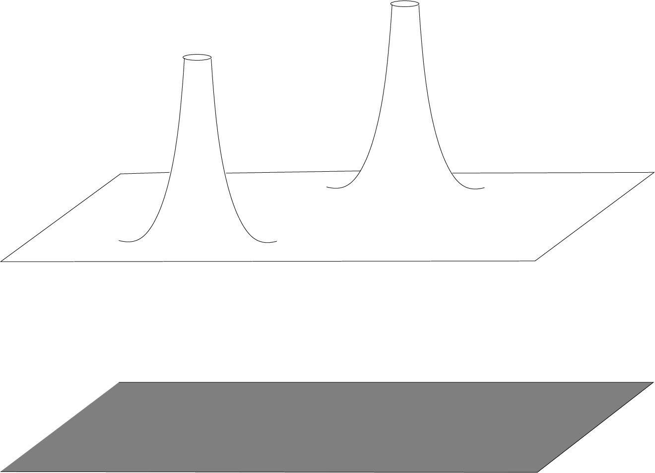
Notice that the probe branes become parallel to the original stack only at infinity: in the interior of the space the probes are curved (see figure 2) and they have a nonvanishing electric field. This field is responsible for breaking eight out of $16$ supersymmetries which would be preserved by the parallel branes. We considered three examples of such setup: D3–D3, D5–D5 systems in type IIB theory and M5–M5 configuration on M theory. In the first two cases the worldvolume flux sources fundamental strings, while in eleven dimensions it mimics M2 branes.

We also looked at other configurations preserving eight supercharges in ten dimensions: they were constructed by putting D3 branes on a D5 geometry or by putting D5 branes on a D3 geometry. In both cases the brane profiles $X({\bf x})$ were governed by the same nonlinear equation

$\displaystyle-(1+(\nabla X)^{2})\partial_{X}H+H\nabla^{2}X+2\nabla H\nabla X=0,$

(2.62)

where $H({\bf x},X)$ was a harmonic function describing the background. The same equation was found to describe a profile of M5’ brane on the M5 geometry (see (2.4)) and for future reference we summarize the harmonic functions for the three situations:

$\displaystyle H_{D3}=1+\frac{Q_{3}}{(X^{2}+{\bf x}_{5}^{2})^{2}},\quad H_{D5}=1+\frac{Q_{5}}{X^{2}+{\bf x}_{3}^{2}},\quad H_{M5}=1+\frac{Q_{M5}}{(X^{2}+{\bf x}_{4}^{2})^{3/2}}.$

(2.63)

Here a subscript of ${\bf x}$ denotes the number of components of this vector. It might be somewhat counterintuitive that positions of supersymmetric probes are described by a nonlinear equation like (2.62): looking at configuration (2.1), one would expect that the branes can be freely superposed. In section 2.4 we will show that this expectation is correct and equation (2.62) can be linearized by a change of variables.

References

• [1] J. Dai, R. G. Leigh and J. Polchinski, Mod. Phys. Lett. A 4, 2073 (1989);
R. G. Leigh, Mod. Phys. Lett. A 4, 2767 (1989);
P. Horava, Nucl. Phys. B 327, 461 (1989); Phys. Lett. B 231, 251 (1989).
• [2] G. T. Horowitz and A. Strominger, Nucl. Phys. B 360, 197 (1991).
• [3] J. Polchinski, Phys. Rev. Lett. 75, 4724 (1995), hep-th/9510017.
• [4] J. M. Maldacena, Adv. Theor. Math. Phys. 2, 231 (1998), Int. J. Theor. Phys. 38, 1113 (1999), hep-th/9711200.
• [5] A. Strominger and C. Vafa, Phys. Lett. B 379, 99 (1996), hep-th/9601029.
• [6] J. McGreevy, L. Susskind and N. Toumbas, JHEP 0006, 008 (2000), hep-th/0003075;
M. T. Grisaru, R. C. Myers and O. Tafjord, JHEP 0008, 040 (2000), hep-th/0008015.
• [7] S. J. Rey and J. T. Yee, Eur. Phys. J. C 22, 379 (2001), hep-th/9803001;
J. Pawelczyk and S. J. Rey, Phys. Lett. B 493, 395 (2000), hep-th/0007154].
• [8] N. Drukker and B. Fiol, JHEP 0502, 010 (2005), hep-th/0501109;
S. Yamaguchi, JHEP 0605, 037 (2006), hep-th/0603208;
J. Gomis and F. Passerini, JHEP 0608, 074 (2006), hep-th/0604007.
• [9] H. Lin, O. Lunin and J. M. Maldacena, JHEP 0410, 025 (2004), hep-th/0409174.
• [10] H. Lin and J. M. Maldacena, Phys. Rev. D 74, 084014 (2006), hep-th/0509235;
J. Gomis and S. Matsuura, JHEP 0706, 025 (2007), arXiv:0704.1657 [hep-th].
• [11] S. Yamaguchi, Int. J. Mod. Phys. A 22, 1353 (2007), hep-th/0601089.
• [12] O. Lunin, JHEP 0606, 026 (2006), hep-th/0604133.
• [13] J. Gomis and C. Romelsberger, JHEP 0608, 050 (2006), hep-th/0604155.
• [14] E. D’Hoker, J. Estes and M. Gutperle, arXiv:0705.1004 [hep-th].
• [15] C. G. . Callan and J. M. Maldacena, Nucl. Phys. B 513, 198 (1998), hep-th/9708147.
• [16] J. P. Gauntlett, arXiv:hep-th/9705011.
• [17] D. J. Smith, Class. Quant. Grav. 20, R233 (2003), hep-th/0210157.
• [18] A. Hanany and E. Witten, Nucl. Phys. B 492, 152 (1997), hep-th/9611230;
E. Witten, Nucl. Phys. B 500, 3 (1997), hep-th/9703166; Nucl. Phys. B 507, 658 (1997), hep-th/9706109;
S. Elitzur, A. Giveon, D. Kutasov, E. Rabinovici and A. Schwimmer, Nucl. Phys. B 505, 202 (1997), hep-th/9704104;
A. Giveon and D. Kutasov, Rev. Mod. Phys. 71, 983 (1999), hep-th/9802067.
• [19] A. Strominger, Phys. Lett. B 383, 44 (1996), hep-th/9512059;
P. K. Townsend, Nucl. Phys. Proc. Suppl. 58, 163 (1997), hep-th/9609217.
• [20] M. Cederwall, A. von Gussich, B. E. W. Nilsson and A. Westerberg, Nucl. Phys. B 490, 163 (1997), hep-th/9610148;
M. Aganagic, C. Popescu and J. H. Schwarz, Phys. Lett. B 393, 311 (1997), hep-th/9610249;
M. Cederwall, A. von Gussich, B. E. W. Nilsson, P. Sundell and A. Westerberg, Nucl. Phys. B 490, 179 (1997), hep-th/9611159;
E. Bergshoeff and P. K. Townsend, Nucl. Phys. B 490, 145 (1997), hep-th/9611173.
• [21] G. T. Horowitz and A. A. Tseytlin, Phys. Rev. D 51, 2896 (1995), hep-th/9409021;
A. A. Tseytlin, Nucl. Phys. B 475, 149 (1996), hep-th/9604035;
A. A. Tseytlin, Class. Quant. Grav. 14, 2085 (1997), hep-th/9702163.
• [22] E. Bergshoeff, E. Sezgin and P. K. Townsend, Phys. Lett. B 189, 75 (1987).
• [23] R. Gueven, Phys. Lett. B 276, 49 (1992).
• [24] M. Perry and J. H. Schwarz, Nucl. Phys. B 489, 47 (1997), hep-th/9611065;
M. Aganagic, J. Park, C. Popescu and J. H. Schwarz, Nucl. Phys. B 496, 191 (1997), hep-th/9701166.
• [25] I. A. Bandos, K. Lechner, A. Nurmagambetov, P. Pasti, D. P. Sorokin and M. Tonin, Phys. Lett. B 408, 135 (1997), hep-th/9703127;
P. Pasti, D. P. Sorokin and M. Tonin, Phys. Lett. B 398, 41 (1997), hep-th/9701037;
I. A. Bandos, K. Lechner, A. Nurmagambetov, P. Pasti, D. P. Sorokin and M. Tonin, Phys. Rev. Lett. 78, 4332 (1997), hep-th/9701149.
• [26] C. Bachas, M. R. Douglas and C. Schweigert, JHEP 0005, 048 (2000), hep-th/0003037.
• [27] J. P. Gauntlett, C. Koehl, D. Mateos, P. K. Townsend and M. Zamaklar, Phys. Rev. D 60, 045004 (1999), hep-th/9903156.
• [28] E. Witten, JHEP 9807, 006 (1998), hep-th/9805112.
• [29] Y. Imamura, Nucl. Phys. B 537, 184 (1999), hep-th/9807179;
C. G. Callan, A. Guijosa and K. G. Savvidy, Nucl. Phys. B 547, 127 (1999), hep-th/9810092;
J. M. Camino, A. V. Ramallo and J. M. Sanchez de Santos, Nucl. Phys. B 562, 103 (1999), hep-th/9905118;
J. Gomis, A. V. Ramallo, J. Simon and P. K. Townsend, JHEP 9911, 019 (1999), hep-th/9907022.
• [30] M. Grana and J. Polchinski, Phys. Rev. D 65, 126005 (2002), hep-th/0106014.
• [31] A. A. Tseytlin, Nucl. Phys. B 469, 51 (1996), hep-th/9602064.
• [32] N. Seiberg and E. Witten, JHEP 9909, 032 (1999), hep-th/9908142.
• [33] A. Hashimoto and N. Itzhaki, Phys. Lett. B 465, 142 (1999), hep-th/9907166.
• [34] J. M. Maldacena and J. G. Russo, JHEP 9909, 025 (1999), hep-th/9908134.
• [35] P. Kraus, F. Larsen and S. P. Trivedi, JHEP 9903, 003 (1999), hep-th/9811120.
• [36] C. V. Johnson, hep-th/0007170.
• [37] J. H. Schwarz, Nucl. Phys. B 226, 269 (1983);
J. H. Schwarz and P. C. West, Phys. Lett. B 126, 301 (1983);
P. S. Howe and P. C. West, Nucl. Phys. B 238, 181 (1984).
• [38] D. Marolf and A. W. Peet, Phys. Rev. D 60, 105007 (1999), hep-th/9903213.
• [39] S. A. Cherkis and A. Hashimoto, JHEP 0211, 036 (2002), hep-th/0210105.
• [40] O. Lunin and S. D. Mathur, Nucl. Phys. B 623, 342 (2002), hep-th/0109154;
O. Lunin, J. M. Maldacena and L. Maoz, arXiv:hep-th/0212210.
• [41] J. B. Gutowski, D. Martelli and H. S. Reall, Class. Quant. Grav. 20, 5049 (2003), hep-th/0306235.
• [42] I. Bena and N. P. Warner, Adv. Theor. Math. Phys. 9, 667 (2005), hep-th/0408106.
• [43] O. Lunin, JHEP 0404, 054 (2004), hep-th/0404006;
S. Giusto, S. D. Mathur and A. Saxena, Nucl. Phys. B 701, 357 (2004), hep-th/0405017; Nucl. Phys. B 710, 425 (2005), hep-th/0406103;
S. Giusto and S. D. Mathur, Nucl. Phys. B 729, 203 (2005), hep-th/0409067
P. Berglund, E. G. Gimon and T. S. Levi, JHEP 0606, 007 (2006), hep-th/0505167.
• [44] O. Lunin, arXiv:0704.3442 [hep-th].
• [45] M. Grana and J. Polchinski, Phys. Rev. D 63, 026001 (2001), hep-th/0009211.