Distance distribution in random graphs and application to networks exploration
Abstract
We consider the problem of determining the proportion of edges that are discovered in an Erdős-Rényi graph when one constructs all shortest paths from a given source node to all other nodes. This problem is equivalent to the one of determining the proportion of edges connecting nodes that are at identical distance from the source node. The evolution of this quantity with the probability of existence of the edges exhibits intriguing oscillatory behavior. In order to perform our analysis, we introduce a new way of computing the distribution of distances between nodes. Our method outperforms previous similar analyses and leads to estimates that coincide remarkably well with numerical simulations. It allows us to characterize the phase transitions appearing when the connectivity probability varies.
pacs
89.75.Hc, 89.20.Hh, 02.50.-r, 05.50.+qI Introduction
The small-world phenomenon has attracted increasing attention over the last few years rand-graphs; milgram. In a small-world network, the average distance between two nodes is small as compared to the total number of nodes. In many natural networks, it is typically of the order of ( is the total number of nodes) and several models have been proposed to explain this phenomenon (see, e.g. rand-graphs; doro2003evolution; watt_sw). In some applications though, one is interested not only in this so-called “average inter-vertex distance”, but in the whole inter-vertex distance distribution.
Even though this distribution is of much interest, it has not
been studied very much in the literature. A theoretical method for
the computation of the distances in uncorrelated random networks
of infinite size has been proposed by Dorogovtsev et al. in 2003
doro_dist. In Fronczak et al. have analyzed the
distance between nodes for a wide class of random networks of
finite size that generalizes the Erdős-Rényi graphs, the so-called
uncorrelated random networks with hidden variables fron.
They propose an approximation of the distribution of the distance
between nodes that performs well for a certain range of the
parameter values. Their formula has the advantage of being simple
and analytical, but the approximations done in the calculations
lead to significative differences with
the numerical evidence for some ranges of the parameters.
Our work is motivated by the analysis of algorithms that have been recently developped for analysing networks, such as the internet. A typical way of doing that is to use the freeware traceroute, that provides the user a short path from his computer to any other one in the internet. In the ASP model (All Shortest Paths), introduced to model this strategy, one chooses a particular node of the network, and then constructs all shortest paths from to all other nodes of the network jlg. Some edges of the network may not belong to any of these shortest paths and so they are left undiscovered. The problem considered in jlg is that of determining the proportion of edges of the network that are discovered. Thus the question is: “what is the proportion of edges that are on at least one shortest path starting from the source?”. As pointed out in jlg, the edges that are not discovered are exactly those connecting nodes that are at identical distances from the source. Indeed, if an edge connects two equidistant nodes, it cannot be on a shortest path from the source, since any path using this edge (say going from to ) can be shortened by going directly to via the shortest path to Conversely, if an edge links two nodes that are not at the same distance, then it links a node at a certain distance to a node at a distance and at least one shortest path to passes through this edge. We are therefore interested in computing the number of edges connecting nodes that are at the same distance from the source. Other models exist for representing network analysis strategies. For instance, jlg introduces the USP model (for Unique Shortest Path). In the USP model one chooses only one shortest path from the source to each node in the graph and so there are possibly more edges that are left undiscovered. Our work is also relevant to the analysis of this model, as it counts the proportion of edges that are never found by any single or multiple USP searches.

In jlg, massive numerical simulations have been performed
to analyze the proportion of edges that are on shortest paths in
Erdős-Rényi graphs. In such random graphs, edges are all equally
likely to be present and the probability of presence is given by
some fixed probability . We do not consider self loops nor
multiple edges. So, for constructing an Erdős-Rényi graph, one needs
to fix two parameters: the number of nodes and the probability
of existence for every edge . As shown in FIG.
1, the proportion of edges that are discovered in
the ASP model presents an interesting dependence in the parameter
. One can directly explain some characteristics of this curve.
When is very small the graph is highly disconnected and
consists in small connected components. Most edges do therefore
not belong to any path starting from the source, and the
proportion of observed edges is close to zero. Conversely, if
is very high, the graph is almost complete, and every shortest
path has length one. So edges are found, while there are
almost edges in the graph, and
thus the proportion also vanishes.
The aims of this paper are first to introduce a new simple model
of inter-vertex distances in Erdős-Rényi graphs that can be used to
compute the curve of FIG. 1 without any numerical
experiment, and second to analyze the oscillating behavior of this
curve and explain the phase transitions appearing with variations
of the graph connectivity. Note that similar oscillating
behaviors in random graphs have recently been observed
holyst-oscillant, and that these phenomena seem to open
challenging questions in random graphs theory. This paper
proposes a precise analysis of such an oscillating behavior in
the simple theoretical framework of Erdős-Rényi graphs. One could
imagine exploiting these oscillations to optimize the design of a
network or to develop method for its analysis, although this is
beyond the scope of this paper. Besides, such applications of the
concepts developed here would probably require some further
analysis and extension of our results, because real networks
often exhibit non-trivial correlations between nodes that do not
occur in Erdős-Rényi graphs. These extensions would however most
likely not lead to the derivation of simple analytical solutions
providing an intuitive understanding of the
phenomena as it is done here.
The remainder of the paper is organized as follows. In Section II, we introduce a recurrence equation allowing to evaluate the inter-vertex distance distribution for Erdős-Rényi graphs, and compare to previously published results fron. From this function we derive a theoretical expression for values shown on FIG. 1. In Section III we analyze this curve, we characterize the phase transitions, and give analytical expressions in different phases (proved in Appendix A). In Section IV we conclude and make some remarks on practical applications of the phenomena studied in the paper.
II Approximation of intervertex distance distribution
In this section we propose an approximation for inter-vertex
distance distribution in Erdős-Rényi graphs. We compare our results to
those obtained by Fronczak et al. fron in a more generic
situation, and show how our results outperform theirs in the
particular case of Erdős-Rényi graphs. We also analyze the accuracy of
our model and its dependence on the graph connectedness. We then
use our inter-vertex distance distribution to estimate the
proportion of equidistant pairs of nodes.
In the sequel, we consider the distance between a randomly selected node and a fixed but initially randomly selected “source node”. Since this source is randomly selected, all results obtained for the distance probability can also be applied to the distance between two randomly selected vertices. Let be the probability for a randomly selected node to be at a distance larger than from the source, that is, the probability that there is no path of length smaller than or equal to from the source to this node. The probability for the node to be at a distance exactly of the source is then given by . Obviously, . We now derive a recurrence relation allowing the computation of for higher values of . A node is at a distance larger than from the source if it is not the source itself, which happens with probability , and if it is connected to no node at distance less than from the source, which happens with probability being the number of nodes at distance less than from the source. We have therefore the following simple relation:
| (1) |
where denotes the probability that . In order to express the probability , we should thus know the distribution of . We approximate this quantity to be always exactly equal to its expectation . Introducing this approximation in (1) we obtain a recurrence relation for
| (2) |
which allows us to compute for any . This formula is
different, but provably equivalent to Equation in
baronchelli06 that has been derived independently for other
purposes.
In fron, Fronczak et al. propose an expression for the intervertex distance distribution of any “random graph with hidden variables”, that are generalizations of Erdős-Rényi graphs. In these graphs, two nodes and are connected with a probability , where each node has its own “hidden variable” and So, in a large graph, the hidden variables represent the expected degree of the vertices. In the particular case of Erdős-Rényi graphs, that is when for all , their expression for the function of inter-vertex distance distribution reduces to:
| (3) |
This result has a straightforward interpretation as the solution
of an other recurrence equation on , although it is not
obtained in that way in fron. A vertex is at a distance
larger than from the source node if all its neighbors are at
distance larger than from the source. Approximating the
number of neighbors by its expectation and neglecting the
dependence effects, one obtains the recurrence . The relation (3) is then re-obtained by
taking as initial
condition. Numerical experiments confirm indeed that taking
or as initial condition has
no influence on the results if is sufficiently large.
 |
 |
| (a) | (b) |
 |
 |
| (c) | (d) |
In FIG. 2 we compare the predictions from the
two models, with numerical results. One can see that both models
perform very well when the average degree is significantly
larger than and if is not too big, as in FIG.
2(c). For an average degree , that is
below the emergence of the giant connected component (see
rand-graphs), our results match approximately the
experimental observations while Fronczak et al.’s model is not
valid as it gives an increasing curve (see FIG.
2(a)). For values of larger than but close
to 1, both models present significant errors but ours is closer to
the experimental observations (see FIG. 2(b)).
Finally, for a large , one can see in FIG.
2(d) that our results match the experimental
data very well while those obtained with the model of
fron are significantly different.
The fact that the model derived in fron behaves very
differently from our model for a certain range of values of
may seem surprising. Our derivation presents indeed various
similarities with the interpretation of Fronczak et al.’s model as
a solution of a recursive equation. Three reasons can however
explain why a model based on this interpretation gives less
accurate results than ours. First, for the possibility
for the randomly selected node to be the source could not be
neglected, as very few nodes are in the connected component of the
source. When is larger than but close to , the
approximation that a node has exactly neighbors leads to
proportionally more important errors. This problem could be solved
by considering a binomial distribution for the number of neighbors
in our interpretation of Fronczak et al.’s model. Finally, for
large values of the number of neighbors of the randomly
selected node is large, so that some independence problems are not
negligible. Indeed, the probabilities for two neighbors of the
randomly selected node to be the source are not independent, as
there is exactly one source in the graph.
The errors of our model, observed for values of larger than
but close to 1 are due to the approximation mentioned above: To
obtain the recurrence equation (2) from
(1), we suppose that the number of vertices at a
distance smaller than from the source is exactly equal to its
expectancy instead of considering its probability
distribution. In this range of parameters, the distribution is far
from being centered because of the existence of a peak around
(see FIG. 3(a)). For these values indeed,
the graph is not totally connected. If the source happens not to
be in the giant connected component, almost all nodes are at an
infinite distance of it, so that is close to for any
. The weight of the peak represents thus the probability for a
randomly selected source not to be in the giant connected
component. It is known that when grows, this probability
tends exponentially to independently of (janson00random, Theorem
5.4). This problem does therefore only appear when
the average degree is very small (but larger than ),
independently of the size of the graph. FIG.
3(b) shows that the problem is already
almost negligible when (for these values, the giant
connected component already contains more than of the
vertices). Note that for the graph is highly disconnected
so that almost no nodes are at a finite distance from the source.
The distribution consists thus only in one peak around
and is therefore centered.
| ||
| (a) | ||
| ||
| (b) |


We close this section by explaining how the distance distribution can be used to compute the proportion of edges belonging to shortest paths starting at the source node. As explained in the introduction, the edges that do not belong to any shortest path are those connecting nodes that are at the same distance from the source, in addition to all edges that are not in the same connected component as the source. Since the expectation of the number of nodes at distance from the source is equal to , the expected number of edges connecting these nodes is roughly equal to . Taking as the total number of edges, we obtain the following expression for the proportion of edges that lie on a shortest path in an Erdős-Rényi graph, which we denote by in the sequel:
| (4) |
Note that this expression implicitly handles the edges that are not in the same connected component as the source if we take . Indeed, this quantity represents those nodes that are not connected to the source, as they are at a distance larger than . The evolutions with of using the two models presented above are represented in FIG. 4 for and . One can see that our results match the experiments very well except when is larger than but close to one, which is the range of parameters for which our model has already been shown to be less accurate. Moreover, the range of values of for which our model is less accurate appears not to grow with .
 |
| (a) |
 |
| (b) |
III Analysis of the curve
In this section we analyze the function generated with
our model and (4). We show the appearance of a
sort of phase transition: for some particular values, a weak
variation of the probability may cause abrupt changes in the
proportion of discovered edges with the ASP model, and affect
dramatically the properties of the graph. We give analytical
formulas for the asymptotic behavior in
several phases.
We begin by analyzing the first transition, starting from small
values of . It is well known rand-graphs that in an
Erdős-Rényi graph, a giant component emerges when becomes larger
than . If the average degree is sufficiently small, the
graph is not connected and the only edges that the observer can
see are in the (small) connected component of the source. This
quantity is negligible in view of the total number of edges, and
so the function is approximately zero. Note however that such
graphs do not contain many cycles, so that most paths starting
from the source are shortest paths. Therefore, the observer
discovers approximately all edges in its connected component. When
grows the size of the connected components increases, so that
more and more edges are discovered. Now when , the
giant component emerges very quickly, and the source is in this
component with a large probability. Since most of the edges are
also in this component, the proportion of discovered edges
increases rapidly with . Simultaneously with the apparition of
a giant component, there also appears a non negligible number of
cycles in the graphs, so that not all edges lie on shortest paths
anymore. As a result of these two conflicting phenomena a (global)
optimum is reached for . Experimentally our model
gives an optimum that seems to lie exactly at but we have
not been able to prove this, nor to express analytically the
values of around However, experiments
seem to indicate that in this range of parameters only
depends on All this can be seen in FIG.
5, for different values of . When
becomes larger, one can see that does not only depend on
, and presents an oscillatory behavior. In particular, the
successive values of the maxima seem to tend to . We
explain
this phenomenon in the sequel.
 |
| (a) |
 |
| (b) |
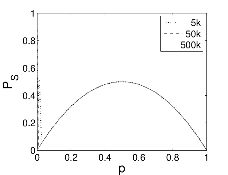
As can be observed in FIG. 6, the shape of tends to the parabola on any interval when increases (note that the -axis is in linear scale). This fact can be proved theoretically, based on our model of evolution of . In the sequel, for the sake of clarity in our analysis, we modify (2), and study the slightly different one:
| (5) |
This new approximation is justified by the fact that we will consider asymptotic behaviors for . Moreover, the results that we derive can be obtained without making this approximation. Observe that , so that . When grows , and if is bounded from below by an arbitrary positive constant tends uniformly to 0. As a consequence the probability for a node to be at a distance from the source tends uniformly to 0 for all except for , for which and . It follows then from (4) that
so that asymptotically, the last maximum of is
and is reached at . The asymptotic parabolic
character of is thus here due to the fact that almost all
nodes tend to be at a distance either 1 or 2 from the source when
grows and is sufficiently large, as can for example be
observed in FIG. 2(d).
We now analyze the oscillating behavior between the first and last
maximum. One can see in FIG. 7 that around
the second rightmost maximum, only depends on
and that asymptotically behaves as
| (6) |
around this maximum. The maximum therefore tends to
when and is attained for
. To explain (6), we
show in the appendix that similarly as above, all nodes are
asymptotically at distance either or when with where are
arbitrarily positive constants.
As in the case of the parabola, this together with (4)
implies that then asymptotically behaves as
We also show that tends to which implies
(6).
 |
| (a) |
 |
| (b) |
Actually the previous relations can be generalized inductively: we prove in the appendix that when with converges uniformly to while all with converge uniformly to 1 and all others to 0. This means that in this range of parameters, and when tends to infinity, almost all nodes are at distance or from the source. It follows then from (4) that
which, as for , is a parabolic curve with respect to .
This parabolic curve attains its maximum when
. So, when ,
contains an unbounded number of oscillations and local
maxima with asymptotic values , and these maxima are
attained when for each as can be seen
on some additional examples in FIG. 8.
Experimentally, all local maxima but the first global one can be
explained in that way. Between two maxima, there is a zone where
asymptotically and , so that
almost all nodes are at distance from the source, and . Such behavior is obtained when with either large values of but still
, or small values of but
still . One can indeed see in FIG.
7 and 8 for example that
the values of the local minima decrease significantly when
increases. Let us mention that an explanation of the oscillatory
behavior based on the fact that almost all nodes are at distance
or from the source had been suggested without proof in
jlg.
 |
| (a) |
 |
| (b) |
IV Conclusions and future work
The goal of this paper was twofold: First, we have proposed a
simple model for the computation of the inter-vertex distance
distribution in a random graph, via a recurrence equation for the
probability for two randomly chosen nodes to be at distance more
than . Contrary to the model of Fronczak et al., our
recurrence equation is not explicitly solvable, but it is more
accurate. It has to be noted that for the range of parameters
corresponding to the oscillating behavior analyzed at the end of
Section III, the two models are equally valid,
and that the analysis that we have made for such values could also
be made using Fronczak et al.’s model. Let us add that the ideas
behind the derivation of the formula remain valid for more general
graphs such as random graphs with hidden variables. In the
particular case of Erdős-Rényi graphs, these ideas lead to a simple
recurrence equation, allowing to compute explicit values
numerically, and to prove the asymptotic behavior of the curve
experimentally obtained in jlg. Nevertheless, a further
analysis for more general graphs could be interesting.
Second, following numerical simulations in previous works
motivated by practical graph exploration questions jlg, we
have analyzed the proportion of edges connecting nodes that are
equidistant from a certain source node in random graphs. The
evolution of this quantity with the parameter exhibits an
intriguing oscillating behavior, which we have been able to
explain and reproduce with a great accuracy using our model. We
have also characterized precisely the (infinite number of)
transitions for this quantity, and the analytical
evolution with in the different phases.
Acknowledgment
The authors wish to thank Renaud Lambiotte for his useful advice.
References
- (1) A. Baronchelli and V. Loreto. Ring structures and mean first passage time in networks. Physical Review E, 73(026103), 2006.
- (2) B. Bollobas. Random Graphs. Cambridge University Press, 2001.
- (3) S.N. Dorogovtsev and J.F.F. Mendes. Evolution of Networks: From Biological Nets to the Internet and WWW. Oxford University Press, Oxford, January 2003.
- (4) S.N. Dorogovtsev, J.F.F. Mendes, and A.N. Samukhin. Metric structure of random networks. Nuclear Physics B, 653(3):307–338, March 2003.
- (5) A. Fronczak, P. Fronczak, and Janusz A. Holyst. Average path length in random networks. Phys. Rev. E, 70, 2004.
- (6) J.-L. Guillaume and M. Latapy. Complex network metrology. Complex Systems, 16:83–94, 2005.
- (7) S. Janson, T. Luczak, and A. Ruci. Random Graphs. Wiley-Interscience, 2000.
- (8) J. Sienkiewicz, P. Fronczak, and J. A. Holyst. Log-periodic oscillations due to discrete effects in complex networks. ArXiv:cond-mat/0608273, 2006.
- (9) J. Travers and S. Milgram. An experimental study of the small world problem. Sociometry, 32(4):425–443, 1969.
- (10) D. J. Watts. Small Worlds: The Dynamics of Networks Between Order and Randomness. Princeton University Press, 2003.
Appendix A Expression of the asymptotic behavior
In this appendix, we provide an analytical expression for when tends to infinity with , and we show that in this range of parameters, almost all nodes are at distance or Suppose first that with for an arbitrary . Then so that uniformly with . From our recurrence formula (5), we have
which, together with the classical relation implies that
| (7) |
holds uniformly for . We now show that
for any two arbitrary constants and This implies that almost all nodes are at distance or from the source. It follows from (7) that is uniformly bounded from below by a positive constant when with , so that we just need to prove the uniform decay of . The latter expression can be rewritten as
| (8) |
Since when with , there uniformly holds
And since it follows from (8) that
which implies the desired result.
There remains to prove our assertions about the asymptotic behavior of for any . We first prove by induction that the two following relations hold uniformly for where is any arbitrary positive constant.
| (9) |
| (10) |
These relations hold for as shown above. Let us now assume that they hold for a certain and prove that they then hold for . Observe first that when with , tends uniformly to 0 and is bounded. It follows then from the induction hypothesis that
uniformly when So Equation (9) is proved. By our recurrence relation (5), . Therefore, there holds
Since is bounded, and since tends thus uniformly to 0 when , the last equation becomes
uniformly for , which proves (10).
Using the results above we now prove that for any , the following holds uniformly
| (11) |
where and are two arbitrary positive constants. By (5), we have
It follows from the results above that is uniformly bounded from below by a positive constant when with , so that we just need to prove the uniform decay of . The latter expression can be rewritten as
| (12) |
Since when with , there uniformly holds
And since when with , it follows from (12) that
which implies the desired result (11).