Quantum decay rates in chaotic scattering

Stéphane Nonnenmacher and Maciej Zworski Address: Service de Physique Théorique, CEA/DSM/PhT, Unité de recherche associé CNRS, CEA/Saclay,
91191 Gif-sur-Yvette, France Email address: nonnen@spht.saclay.cea.fr Address: Mathematics Department, University of California
Evans Hall, Berkeley, CA 94720, USA Email address: zworski@math.berkeley.edu

1. Statement of Results

In this article we prove that for a large class of operators, including Schrödinger operators,

(1.1)

P(h)=-h^{2}\Delta+V(x)\,,\ \ V\in{\mathcal{C}}^{\infty}_{\rm{c}}(X)\,,\ \ X={\mathbb{R}}^{2}\,,

with hyperbolic classical flows, the smallness of dimension of the trapped set implies that there is a gap between the resonances and the real axis. In other words, the quantum decay rates are bounded from below if the classical repeller is sufficiently filamentary. The higher dimensional statement is given in terms of the topological pressure and is presented in Theorem 3. Under the same assumptions, we also prove a useful resolvent estimate:

(1.2)

\|\chi(P(h)-E)^{-1}\chi\|_{L^{2}\rightarrow L^{2}}\leq C\,\frac{\log(1/h)}{h}\,,

for any compactly supported bounded function $\chi$ - see Theorem 5, and a remark following it for an example of applications.

We refer to §3.2 for the general assumptions on $P(h)$ , keeping in mind that they apply to $P(h)$ of the form (1.1). The resonances of $P(h)$ are defined as poles of the meromorphic continuation of the resolvent:

R(z,h)\stackrel{{\scriptstyle\rm{def}}}{{=}}(P(h)-z)^{-1}\;:\;L^{2}(X)\longrightarrow L^{2}(X)\,,\ \ \mathop{\rm Im}\nolimits z>0\,,

through the continuous spectrum $[0,\infty)$ . More precisely,

R(z,h)\;:\;L^{2}_{\rm{comp}}(X)\longrightarrow L^{2}_{\rm{loc}}(X)\,,\ \ z\in{\mathbb{C}}\setminus(-\infty,0]\,,

is a meromorphic family of operators (here $L^{2}_{\rm{comp}}$ and $L^{2}_{\rm{loc}}$ denote functions which are compactly supported and in $L^{2}$ , and functions which are locally in $L^{2}$ ). The poles are called resonances and their set is denoted by $\operatorname{Res}(P(h))$ — see [4, 46] for introduction and references. Resonances are counted according to their multiplicities (which is generically one [22]).

In the case of (1.1) the classical flow is given by Newton’s equations:

\displaystyle\begin{gathered}\Phi^{t}(x,\xi)\stackrel{{\scriptstyle\rm{def}}}{{=}}(x(t),\xi(t))\,,\\ x^{\prime}(t)=\xi(t)\,,\ \ \xi^{\prime}(t)=-dV(x(t))\,,\ \ x(0)=x\,,\ \ \xi(0)=\xi\,.\end{gathered}

This flow preserves the classical Hamiltonian

p(x,\xi)\stackrel{{\scriptstyle\rm{def}}}{{=}}|\xi|^{2}+V(x)\,,\ \ (x,\xi)\in T^{*}X\,,\ \ X={\mathbb{R}}^{2}\,,

and the energy layers of $p$ are denoted as follows:

(1.5)

{\mathcal{E}}_{E}\stackrel{{\scriptstyle\rm{def}}}{{=}}\left\{\,\rho\in T^{*}X,\ p(\rho)=E\,\right\},\qquad{\mathcal{E}}_{E}^{\delta}\stackrel{{\scriptstyle\rm{def}}}{{=}}\bigcup_{|E^{\prime}-E|<\delta}{\mathcal{E}}_{E^{\prime}}\,,\quad\delta>0\,.

The incoming and outgoing sets at energy $E$ are defined as

(1.6)

\Gamma^{\pm}_{E}\stackrel{{\scriptstyle\rm{def}}}{{=}}\left\{\,\rho\in T^{*}X\;:\;p(\rho)=E\,,\ \ \Phi^{t}(\rho)\not\rightarrow\infty\,,\ t\rightarrow\mp\infty\,\right\}\subset{\mathcal{E}}_{E}\,.

The trapped set at energy $E$ ,

(1.7)

K_{E}\stackrel{{\scriptstyle\rm{def}}}{{=}}\Gamma^{+}_{E}\cap\Gamma^{-}_{E}

is a compact, locally maximal invariant set, contained inside $T^{*}_{B(0,R_{0})}X$ , for some $R_{0}$ . That is clear for (1.1) but also follows from the general assumptions of §3.2.

We assume that the flow $\Phi^{t}$ is hyperbolic on $K_{E}$ .

The definition of hyperbolicity is recalled in (3.17) – see §3.2 below. We recall that it is a structurally stable property, so that the flow is then also hyperbolic on $K_{E^{\prime}}$ , for $E^{\prime}$ near $E$ . Classes of potentials satisfying this assumption at a range of non-zero energies are given in [27], [37, Appendix c], [44], see also Fig.1.

Refer to caption — Figure 1. A three bump potential exhibiting a hyperbolic trapped set for a range of energies. When the curve $\{V=E\}$ is made of three approximate circles of radii $a$ and centers at equilateral distance $R$ , the partial dimension $d_{H}$ in (1.9) is approximately $\log 2/\log(R/a)$ when $R\gg a$ .

The dimension of the trapped set appears in the fractal upper bounds on the number of resonances. We recall the following result [41] (see [37] for the first result of this type):

Theorem 1.

Let $P(h)$ be given by (1.1) and suppose that the flow $\Phi^{t}$ is hyperbolic on $K_{E}$ . Then in the semiclassical limit

(1.8)

|\operatorname{Res}(P(h))\cap D(E,Ch)|={\mathcal{O}}(h^{-d_{H}})\,,

where

(1.9)

2d_{H}+1=\text{ Hausdorff dimension of $K_{E}$.}

We note that using [33, Theorem 4.1], and in dimension $n=2$ , we strengthened the formulation of the result in [41] by replacing upper Minkowski (or box) dimension by the Hausdorff dimension. We refer to [41, Theorem 3] for the slightly more cumbersome general case.

In this article we address a different question which has been present in the physics literature at least since the seminal paper by Gaspard and Rice [15]. In the same setting of scattering by several convex obstacles, it has also been considered around the same time by Ikawa [19] (see also the careful analysis by Burq [6] and a recent paper by Petkov and Stoyanov [34]).

Question: What properties of the flow $\Phi_{t}$ , or of $K_{E}$ alone, imply the existence of a gap $\gamma>0$ such that, for $h>0$ sufficiently small,

$z\in\operatorname{Spec}(P(h))\,,\quad\mathop{\rm Re}\nolimits z\sim E\;\Longrightarrow\;\mathop{\rm Im}\nolimits z<-\gamma h\,?$

In other words, what dynamical conditions guarantee a lower bound on the quantum decay rate?

Numerical investigations in different settings of semiclassical three bump potentials [23, 24], three disk scattering [15, 25, 45], Cantor-like Julia sets for $z\mapsto z^{2}+c$ , $c<-2$ [42], and quantum maps [31, 35], all indicate that a trapped set $K_{E}$ of low dimension (a “filamentary” fractal set) guarantees the existence of a resonance gap $\gamma>0$ .

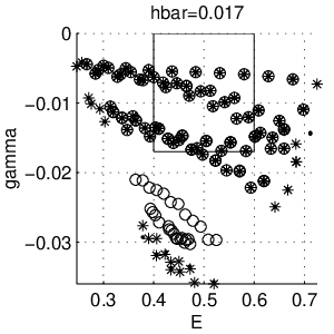
Some of these works also confirm the fractal Weyl law of Theorem 1. which, unlike Theorem 2 below, was first conjectured in the mathematical works on counting resonances.

Here we provide the following

Theorem 2.

Suppose that the assumptions of Theorem 1 hold and that the dimension $d_{H}$ defined in (1.9) satisfies

(1.10)

d_{H}<\frac{1}{2}\,.

Then there exists $\delta,\ \gamma>0$ , and $h_{\delta,\gamma}>0$ such that

(1.11)

0<h<h_{\delta,\gamma}\ \Longrightarrow\ \operatorname{Res}(P(h))\cap\left([E-\delta,E+\delta]-i[0,h\gamma]\right)=\emptyset\,.

The statement of the theorem can be made more general and more precise using a more sophisticated dynamical object, namely the topological pressure of the flow on $K_{E}$ with respect to the unstable Jacobian:

{\mathcal{P}}_{E}(s)=\text{ pressure of the flow on $K_{E}$ with respect to the unstable Jacobian.}

We will give two equivalent definitions of the pressure below, the simplest to formulate (but not to use), given in (3.24).

The main result of this paper is

Theorem 3.

Suppose that $P(h)$ satisfies the general assumptions of §3.2 (in particular it can be of the form (1.1) with $X={\mathbb{R}}^{n}$ ), and that the flow $\Phi^{t}$ is hyperbolic on the trapped set $K_{E}$ . Suppose that the topological pressure satisfies

{\mathcal{P}}_{E}(1/2)<0\,.

Then there exists $\delta>0$ such that for any $\gamma$ satisfying

(1.12)

0<\gamma<\min_{|E-E^{\prime}|\leq\delta}(-{\mathcal{P}}_{E^{\prime}}(1/2))\,,

there exits $h_{\delta,\gamma}>0$ such that

(1.13)

0<h<h_{\delta,\gamma}\ \Longrightarrow\ \operatorname{Res}(P(h))\cap\left([E-\delta,E+\delta]-i[0,h\gamma]\right)=\emptyset\,.

For $n=2$ , $d_{H}<1/2$ is equivalent to ${\mathcal{P}}_{E}(1/2)<0$ , which shows that Theorem 2 follows from Theorem 3. The connection between ${\rm sgn}{\mathcal{P}}_{E}(1/2)$ and a resonance gap also holds in dimension $n\geq 3$ ; however, for $n\geq 3$ there is generally no simple link between the sign of ${\mathcal{P}}_{E}(1/2)$ and the value of $d_{H}$ (except when the flow is “conformal” in the unstable, respectively stable directions [33]).

The optimality of Theorem 3 is not clear. Except in some very special cases (for instance when $K_{E}$ consists of one hyperbolic orbit) we do not expect the estimate on the width of the resonance free region in terms of the pressure to be optimal. In fact, in the analogous case of scattering on convex co-compact hyperbolic surfaces the results of Naud (see [29] and references given there) show that the resonance free strip is wider at high energies than the strip predicted by the pressure. That relies on delicate zeta function analysis following the work of Dolgopyat: at zero energy there exists a Patterson-Sullivan resonance with the imaginary part (width) given by the pressure, but all other resonances have more negative imaginary parts. A similar phenomenon occurs in the case of Euclidean obstacle scattering as has recently been shown by Petkov and Stoyanov [34].

The proof of Theorem 3 is based on the ideas developed in the recent work of Anantharaman and the first author [2, 3] on semiclassical defect measures for eigenfuctions of the Laplacian on manifolds with Anosov geodesic flows. Although we do not use semiclassical defect measures in the proof of Theorem 3, the following result provides a connection:

Theorem 4.

Let $P(h)$ satisfy the general assumptions of §3.2 (no hyperbolicity assumption here). Consider a sequence of values $h_{k}\to 0$ and a corresponding sequence of resonant states (see (3.4) in §3.2 below) satisfying

(1.14)

\|u(h_{k})\|_{L^{2}(\pi(K_{E})+B(0,\delta))}=1\,,\ \ \mathop{\rm Re}\nolimits z(h_{k})=E+o(1)\,,\ \ \mathop{\rm Im}\nolimits z(h)\geq-Ch

where $K_{E}$ is the trapped set at energy $E$ (1.7) and $\delta>0$ . Suppose that a semiclassical defect measure $d\mu$ on $T^{*}X$ is associated with the sequence $(u(h_{k}))$ :

\displaystyle\begin{gathered}\langle a^{w}(x,h_{k}D)\chi u(h_{k}),\chi u(h_{k})\rangle\longrightarrow\int_{T^{*}X}a(\rho)\,d\mu(\rho)\,,\ \ k\rightarrow\infty\,,\\ a\in{\mathcal{C}}^{\infty}_{\rm{c}}(T^{*}X)\,,\ \ \chi\in{\mathcal{C}}^{\infty}_{\rm{c}}(X)\,,\ \ \pi^{*}\chi|_{\operatorname{supp}a}\equiv 1\,,\ \ \pi:T^{*}X\rightarrow X\,.\end{gathered}

Then

(1.17)

\operatorname{supp}\mu\subset\Gamma^{+}_{E}

and there exists $\lambda>0$ such that

(1.18)

\lim_{k\rightarrow\infty}\mathop{\rm Im}\nolimits z(h_{k})/h_{k}=-\lambda/2\,,\quad\text{ and}\quad{\mathcal{L}}_{H_{p}}\mu=\lambda\mu\,.

See Fig. 3 for a numerical result illustrating the theorem. A similar analysis of the phase space distribution for the resonant eigenstates of quantized open chaotic maps (discrete-time models for scattering Hamiltonian flows) has been recently performed in [21, 30]. Connecting this theorem with Theorems 2 and 3, we see that the semiclassical defect measures associated with sequences of resonant states have decay rates $\lambda$ bounded from below by $2\gamma>0$ , once the dimension of the trapped set is small enough ( $n=2$ ), or more generally, the pressure at $\frac{1}{2}$ is negative.

Our last result is the precise version of the resolvent estimate (1.2):

Theorem 5.

(1.19)

\|\chi(P(h)-E)^{-1}\chi\|_{L^{2}(X)\rightarrow L^{2}(X)}\leq C\,\frac{\log(1/h)}{h}\,,\quad 0<h<h_{0}\,.

Notice that the upper bound $C\,\log(1/h)/h$ is the same as in the one obtained in the case of one hyperbolic orbit by Christianson [8]. To see how results of this type imply dynamical estimates see [7, 8]. In the context of Theorem 5, the applications are presented in [9]. Referring to that paper for details and pointers to the literatures we present one application.

Let $P=-h^{2}\Delta_{g}$ be the Laplace-Bertrami operator satisfying the assumptions below, for instance on a manifold Euclidean outside of a compact set with the standard metric there. The Schrödinger propagator, $\exp(-it\Delta_{g})$ , is unitary on any Sobolev space so regularity is not improved in propagation. Remarkably, when $K=\emptyset$ , that is, when the metric is nontrapping, the regularity improves when we integrate in time and cut-off in space:

\int_{0}^{T}\|\chi\exp(-it\Delta_{g})u\|_{H^{1/2}(X)}^{2}dt\leq C\|u\|_{L^{2}(X)}^{2}\,,\ \ \ \chi\in C^{\infty}_{\rm{c}}(X)\,,

and this much exploited effect is known as local smoothing. As was shown by Doi [12] any trapping (for instance a presence of closed geodesics or more generally $K\neq\emptyset$ ) will destroy local smpoothing. Theorem 5 implies that under the assumptions that the geodesic flow is hyperbolic on the trapped set $K\subset S^{*}X$ , and that the pressure is negative at $1/2$ (or, when $\dim X=2$ , that the dimension of $K\subset S^{*}X$ is less than $2$ ) local smoothing holds with $H^{1/2}$ replaced by $H^{1/2-\epsilon}$ for any $\epsilon>0$ .

Notation. In the paper $C$ denotes a constant the value of which may changes from line to line. The constants which matter and have to be balanced against each other will always have a subscript $C_{1},C_{2}$ and alike. The notation $u={\mathcal{O}}_{V}(f)$ means that $\|u\|_{V}={\mathcal{O}}(f)$ , and the notation $T={\mathcal{O}}_{V\rightarrow W}(f)$ means that $\|Tu\|_{W}={\mathcal{O}}(f)\|u\|_{V}$ .

2. Outline of the proof

It this section we present the main ideas whith the precise definitions and references to previous works given in the main body of the paper. The operator to keep in mind is $P=P(h)=-h^{2}\Delta_{g}+V$ , where $V\in{\mathcal{C}}^{\infty}_{\rm{c}}(X)$ , $X={\mathbb{R}}^{n}$ , and the metric $g$ is Euclidean outside a compact set. The corresponding classical Hamiltonian is given by $p=\xi^{2}+V(x)$ . Weaker assumptions, which in particular do not force the compact support of the perturbation, are described in §3.2.

First we outline the proof of Theorem 3 in the simplified case in which resonances are replaced by the eigenvalues of an operator modified by a complex absorbing potential:

P_{W}=P_{W}(h)\stackrel{{\scriptstyle\rm{def}}}{{=}}P-iW\,,

where $W\in{\mathcal{C}}^{\infty}(X;[0,1])$ , satisfies the following conditions:

W\geq 0\,,\qquad\operatorname{supp}W\subset X\setminus B(0,R_{1})\,,\qquad W|_{X\setminus B(0,R_{1}+r_{1})}=1\,,

for $R_{1},r_{1}$ sufficiently large. In particular, $R_{1}$ is large enough so that $\pi(K_{E})\subset B(0,R_{1})$ , where $K_{E}$ is the trapped set given by (1.7). The non-self-adjoint operator $P_{W}$ has a discrete spectrum in $\mathop{\rm Im}\nolimits z>-1/C$ and the analogue of Theorem 3 reads:

Theorem 3^′.Under the assumptions of Theorem 3, for

(2.1)

0<\gamma<\min_{|E-E^{\prime}|\leq\delta}(-{\mathcal{P}}_{E^{\prime}}(1/2))\,,

there exits $h_{0}=h_{0}(\gamma,\delta)$ such that for $0<h<h_{0}$ ,

(2.2)

\operatorname{Spec}(P_{W}(h))\cap\left([E-\delta,E+\delta]-i[0,h\gamma]\right)=\emptyset\,.

This means that the spectrum of $P_{W}(h)$ near $E$ is separated from the real axis by $h\gamma$ , where $\gamma$ is given in terms of the pressure of the square root of the unstable Jacobian, ${\mathcal{P}}_{E}(1/2)$ .

This spectral gap is equivalent to the fact that the decay rate of any eigenstate is bounded from below:

P_{W}\,u=z\,u\,,\ \ z\in D(E,1/C)\,,\ \ u\in L^{2}\ \Longrightarrow\ \|\exp(-itP_{W}/h)u\|\leq e^{-\gamma t}\,\|u\|\,.

This is the physical meaning of the gap between the spectrum (or resonances) and the real axis — a lower bound for the quantum decay rate — and the departing point for the proof. To show (2.2) we will show that for functions, $u$ , which are microlocally concentrated near the energy layer ${\mathcal{E}}_{E}=p^{-1}(E)$ (that is, $u=\chi^{w}(x,hD)u+{\mathcal{O}}(h^{\infty})$ for a $\chi$ supported near ${\mathcal{E}}_{E}$ ) we have

\displaystyle\begin{gathered}\|e^{-itP_{W}/h}u\|\leq C\,h^{-n/2}\,e^{-\lambda t}\,\|u\|\,,\qquad 0<\lambda<\min_{|E-E^{\prime}|\leq\delta}(-{\mathcal{P}}_{E^{\prime}}(1/2))\,,\\ 0\leq t\leq\widetilde{M}\log(1/h)\,,\end{gathered}

for any $\widetilde{M}$ . Taking $\widetilde{M}\gg n/2\lambda$ and applying the estimate to an eigenstate $u$ gives (2.2).

To prove (2) we decompose the propagator using an open cover $(W_{a})_{a\in A}$ of the neighbourhood ${\mathcal{E}}_{E}^{\delta}$ of the energy surface. That cover is adapted to the definition of the pressure (see §§5.2,5.3) and it leads to a microlocal partition of a neighbourhood of the energy surface:

\sum_{a\in A}\Pi_{a}=\chi^{w}(x,hD)+{\mathcal{O}}(h^{\infty})\,,\quad\chi\equiv 1\ \text{ on ${\mathcal{E}}_{E}^{\delta/8}$},\quad\text{ess-supp}\;\Pi_{a}\Subset W_{a}\,.

The definition of the pressure in §5.2 also involves a time $t_{0}>1$ , independent of $h$ , but depending on the classical cover. Taking

(2.5)

N\leq M\log(1/h)\,\qquad N\in{\mathbb{N}},\qquad M>0\ \text{fixed but arbitrary large},

the propagator at time $t=N\,t_{0}$ acting of functions $u$ microlocalized inside ${\mathcal{E}}_{E}^{\delta/8}$ can be written as

(2.6)

e^{-iNt_{0}P_{W}/h}\,u=\sum_{\alpha\in A^{N}}U_{\alpha_{N}}\circ\cdots\circ U_{\alpha_{1}}\,u+{\mathcal{O}}(h^{\infty})\,\|u\|\,,\qquad U_{a}\stackrel{{\scriptstyle\rm{def}}}{{=}}e^{-it_{0}P_{W}/h}\,\Pi_{a}\,.

Most terms in the sum appearing on the right hand side of (2.6) are negligible. The sequences $\alpha=(\alpha_{1},\cdots,\alpha_{N})$ which are classically forbidden, that is, for which the corresponding sequences of neighbourhoods are not successively connected by classical propagation in time $t_{0}$ , lead to negligible terms. So do the sequences for which the propagation crosses the region where $W=1$ : the operator $\exp(-it_{0}P_{W}/h)$ is negligible there, due to damping (or “absorption”) by $W$ .

As a result, the only terms relevant in the sum on the right hand side of (2.6) come from $\alpha\in A_{1}^{N}\cap{\mathcal{A}}_{N}$ where $A_{1}$ indexes the element of the partition intersecting the trapped set $K_{E}$ , and ${\mathcal{A}}_{N}$ are the classically allowed sequences — see (6.29). We then need the crucial hyperbolic dispersion estimate proved in §7 after much preliminary work in §§4.3 and 5.1: for $N\leq M\log(1/h)$ , $M>0$ arbitrary, we have for any sequence $\alpha\in A_{1}^{N}\cap{\mathcal{A}}_{N}$ :

(2.7)

\|U_{\alpha_{N}}\circ\cdots\circ U_{\alpha_{1}}\|\leq h^{-n/2}(1+\epsilon_{0})^{N}\prod_{j=1}^{N}\left(\inf_{\rho\in W_{\alpha_{j}}\cap K^{\delta}_{E}}\det\big(d\Phi^{t_{0}}(\rho)|_{E^{+0}_{\rho}}\big)\right)^{-\frac{1}{2}}\,.

The expression in parenthesis is the coarse-grained unstable Jacobian defined in (5.22), and $\epsilon_{0}>0$ is a parameter depending on the cover $(W_{a})$ , which can be taken arbitrarily small — see (5.24). From the definition of the pressure in §5.2, summing (2.7) over $\alpha\in A_{1}^{N}\cap{\mathcal{A}}_{N}$ leads to (2), with $\widetilde{M}=Mt_{0}$ .

In §9 we show how to use (2) to obtain a resolvent estimate for $P_{W}$ : at an energy $E$ for which the flow is hyperbolic on $K_{E}$ and ${\mathcal{P}}_{E}(1/2)<0$ , we have

(2.8)

\|(P_{W}-E)^{-1}\|_{L^{2}(X)\rightarrow L^{2}(X)}\leq C\,\frac{\log(1/h)}{h}\,,\qquad 0<h<h_{0}\,.

To prove Theorem 3, that is the gap between resonances and the real axis, we use the complex scaled operator $P_{\theta}$ : its eigenvalues near the real axis are resonances of $P$ . If $V$ is a decaying real analytic potential extending to a conic neighbourhood of ${\mathbb{R}}^{n}$ (for instance a sum of three Gaussian bumps showed in Fig. 1), then we can take $P_{\theta}=-h^{2}e^{-2i\theta}\Delta+V(e^{i\theta}x)$ , though in this paper we will always use exterior complex scaling reviewed in §3.4, with $\theta\simeq M_{1}\log(1/h)/h$ , where $M_{1}$ is chosen depending on $M$ in (2.5).

To use the same strategy of estimating $\exp(-itP_{\theta}/h)$ we need to further modify the operator by conjugation with microlocal exponential weights. That procedure is described in §6. The methods developed there are also used in the proof of Theorem 4 and in showing how the estimate (2.8) implies Theorem 5.

Since we concentrate on the more complicated, and scientifically relevant, case of resonances, the additional needed facts about the study of $P_{W}$ and its propagator are presented in the Appendix.

3. Preliminaries and Assumptions

In this section we recall basic concepts of semiclassical analysis, state the general assumptions on operators to which the theorems above apply, define hyperbolicity and topological pressure. We also define resonances using complex scaling which is the standard tool in the study of their distribution. Finally, we will review some results about semiclassical Lagrangian states and Fourier integral operators.

3.1. Semiclassical analysis

Let $X$ be a ${\mathcal{C}}^{\infty}$ manifold which agrees with ${\mathbb{R}}^{n}$ outside a compact set, or more generally

X=X_{0}\sqcup({\mathbb{R}}^{n}\setminus B(0,R_{0}))\sqcup\cdots\sqcup({\mathbb{R}}^{n}\setminus B(0,R_{0}))\,,\ \ X_{0}\Subset X\,.

A weight function on $T^{*}X$ is of the form

m:T^{*}X\longrightarrow(0,\infty)\,,\ \ m(x,\xi)\leq C(1+d(x,y)+|\xi-\eta|)^{N}m(y,\eta)\,,

where $d(x,y)$ is a distance function on $X$ , and any uniform choice of distance in the fibers is allowed — the usual Euclidean distance is taken outside $X_{0}$ . The typical choice is $m(x,\xi)=1+|\xi|^{2}_{g}$ , for a metric $g$ .

The class of symbols associated to the weight $m$ is defined as

S^{k}_{\delta}(T^{*}X,m)=\left\{\,a\in{\mathcal{C}}^{\infty}(T^{*}X\times(0,1]):|\partial_{x}^{\alpha}\partial_{\xi}^{\beta}a(x,\xi;h)|\leq C_{\alpha}m(x,\xi)h^{-k-\delta(|\alpha|+|\beta|).}\,\right\}\,.

Most of the time we will use the class with $\delta=0$ in which case that we drop the subscript. When $m\equiv 1$ and $k=0$ , we simply write $S(T^{*}X)$ or $S$ for the class of symbols.

We denote by $\Psi_{h,\delta}^{k}(X,m)$ or $\Psi_{h}^{k}(X,m)$ the corresponding class of pseudodifferential operators. We have surjective quantization and symbol maps:

\operatorname{Op}\;:\;S^{k}(T^{*}X,m)\ \longrightarrow\Psi^{k}_{h}(X,m)\,,\quad\sigma_{h}\;:\;\Psi_{h}^{k}(X,m)\ \longrightarrow S^{k}(T^{*}X,m)/S^{k-1}(T^{*}X,m)\,.

Multiplication of symbols corresponds to composition of operators, to leading order:

\sigma_{h}(A\circ B)=\sigma_{h}(A)\sigma_{h}(B)\,,

and

\sigma_{h}\circ\operatorname{Op}:S^{k}(T^{*}X,m)\ \longrightarrow S^{k}(T^{*}X,m)/S^{k-1}(T^{*}X,m)\,,

is the natural projection map. A finer filtration can be obtained by combining semiclassical calculus with the standard calculus (or in the yet more general framework of the Weyl calculus) — see for instance [40, §3].

The class of operators and the quantization map are defined locally using the definition on ${\mathbb{R}}^{n}$ :

(3.1)

\operatorname{Op}(a)u(x^{\prime})=a^{w}(x,hD)u(x^{\prime})=\frac{1}{(2\pi h)^{n}}\int\int a\big(\frac{x^{\prime}+x}{2},\xi\big)e^{i\langle x^{\prime}-x,\xi\rangle/h}u(x)dxd\xi\,,

and we refer to [11, Chapter 7] for a detailed discussion, and to [13, Appendix D.2] for the semiclassical calculus on manifolds.

The semiclassical Sobolev spaces, $H_{h}^{s}(X)$ are defined by choosing a globally elliptic, self-adjoint operator, $A\in\Psi_{h}(X,\langle\xi\rangle)$ (that is an operator satisfying $\sigma(A)\geq\langle\xi\rangle/C$ everywhere) and putting

\|u\|_{H_{h}^{s}}=\|A^{s}u\|_{L^{2}(X)}\,.

When $X={\mathbb{R}}^{n}$ ,

\|u\|^{2}_{H_{h}^{s}}\sim\int_{{\mathbb{R}}^{n}}\langle\xi\rangle^{2s}|{\mathcal{F}}_{h}u(\xi)|^{2}d\xi\,,\ \ \ {\mathcal{F}}_{h}u(\xi)\stackrel{{\scriptstyle\rm{def}}}{{=}}\frac{1}{(2\pi h)^{n/2}}\int_{{\mathbb{R}}^{n}}u(x)e^{-i\langle x,\xi\rangle/h}dx\,.

Unless otherwise stated all norms in this paper, $\|\bullet\|$ , are $L^{2}$ norms.

For $a\in S(T^{*}X)$ we follow [40] and say that the essential support is equal to a given compact set $K\Subset T^{*}X$ ,

{\text{ess-supp}}_{h}\;a=K\Subset T^{*}X\,,

if and only if

\forall\,\chi\in S(T^{*}X)\,,\ \operatorname{supp}\chi\subset\complement K\ \Longrightarrow\ \chi\,a\in h^{\infty}{\mathcal{S}}(T^{*}X)\,.

Here ${\mathcal{S}}$ denotes the Schwartz class which makes sense since $X$ is Euclidean outside a compact. In this article we are only concerned with a purely semiclassical theory and deal only with compact subsets of $T^{*}X$ .

For $A\in\Psi_{h}(X)$ , $A=\operatorname{Op}(a)$ , we put

\operatorname{WF}_{h}(A)=\text{ess-supp}_{h}\;a\,,

noting that the definition does not depend on the choice of $\operatorname{Op}$ .

We introduce the following condition

(3.2)

u\in{\mathcal{C}}^{\infty}((0,1]_{h};{\mathcal{D}}^{\prime}(X))\,,\ \ \ \exists\;P\,,h_{0}\,,\ \ \|\langle x\rangle^{-P}u\|_{L^{2}(X)}\leq h^{-P}\,,\ h<h_{0}\,,

and call families, $u=u(h)$ , satisfying (3.2) $h$ -tempered. What we need is that for $u(h)$ , $h$ -tempered, $\chi^{w}(x,hD)u(h)\in h^{\infty}{\mathcal{S}}(X)$ for $\chi\in h^{\infty}{\mathcal{S}}(T^{*}X)$ . That is, applying an operator in the residual class produces a negligible contribution.

For such $h$ -tempered families we define the semiclassical $L^{2}$ -wave front set :

(3.3)

\operatorname{WF}_{h}(u)=\complement\big\{(x,\xi)\;:\;\exists\,a\in S(T^{*}X)\,,\ \ a(x,\xi)\neq 0\,,\ \|a^{w}(x,hD)u\|_{L^{2}}={\mathcal{O}}(h^{\infty})\big\}\,.

The last condition in the definition can be equivalently replaced with

a^{w}(x,hD)u\in h^{\infty}{\mathcal{C}}^{\infty}((0,1]_{h};{\mathcal{C}}^{\infty}(X))\,,

since we may always take $a\in{\mathcal{S}}(T^{*}X)$ .

Equipped with the notion of semiclassical wave front set, it is useful and natural to consider the operators and their properties microlocally. For that we consider the classe of tempered operators, $T=T(h)\;:\;{\mathcal{S}}(X)\rightarrow{\mathcal{S}}^{\prime}(X)$ , defined by the condition

\exists\,P,h_{0}\,,\qquad\|\langle x\rangle^{-P}Tu\|_{H_{h}^{-P}(X)}\leq h^{-P}\|\langle x\rangle^{P}u\|_{H_{h}^{P}(X)}\,,\ \ 0<h<h_{0}\,.

For open sets, $V\subset\overline{V}\Subset T^{*}X$ , $U\subset\overline{U}\Subset T^{*}X$ , the operators defined microlocally near $V\times U$ are given by the following equivalence classes of tempered operators:

\displaystyle\begin{gathered}T\sim T^{\prime}\ \text{if and only if there exist open sets}\\ \widetilde{U},\,\widetilde{V}\Subset T^{*}X,\ \ \overline{U}\Subset\widetilde{U},\ \ \overline{V}\Subset\widetilde{V},\ \ \text{such that}\\ A(T-T^{\prime})B={\mathcal{O}}_{{{\mathcal{S}}}^{\prime}\to{{\mathcal{S}}}}(h^{\infty})\,,\\ \text{for any }A,B\in\Psi_{h}(X)\ \ \text{with }\quad\operatorname{WF}_{h}(A)\subset\widetilde{V}\,,\ \ \operatorname{WF}_{h}(B)\subset\widetilde{U}\,.\\ \end{gathered}

For two such operators $T,T^{\prime}$ we say that $T=T^{\prime}$ microlocally near $V\times U$ . If we assumed that, say $A=a^{w}(x,hD)$ , where $a\in{\mathcal{C}}^{\infty}_{\rm{c}}(T^{*}X)$ then ${\mathcal{O}}_{{\mathcal{S}}^{\prime}\to{\mathcal{S}}}(h^{\infty}),$ could be replaced by ${\mathcal{O}}_{L^{2}\to L^{2}}(h^{\infty})$ in the condition. We should stress that “microlocally” is always meant in this semi-classical sense in our paper.

The operators in $\Psi_{h}(X)$ are bounded on $L^{2}$ uniformly in $h$ . For future reference we also recall the sharp Gårding inequality (see for instance [11, Theorem 7.12]):

(3.9)

a\in S(T^{*}X)\,,\quad a\geq 0\ \Longrightarrow\ \langle a^{w}(x,hD)u,u\rangle\geq-Ch\|u\|_{L^{2}}^{2}\,,\quad u\in L^{2}(X)\,,

and Beals’s characterization of pseudodifferential operators on $X$ (see [11, Chapter 8] and [41, Lemma 3.5] for the $S_{\delta}$ case) :

(3.10)

A\in\Psi_{h,\delta}(X)\;\Longleftrightarrow\;\left\{\begin{array}[]{l}\|\operatorname{ad}_{W_{N}}\cdots\operatorname{ad}_{W_{1}}A\|_{L^{2}\rightarrow L^{2}}={\mathcal{O}}(h^{(1-\delta)N})\\ \\ \ \forall\,W_{j}\in{\rm{Diff}}^{1}(X)\,,\quad j=1,\cdots,N\,,\\ \\ \text{$W_{j}=\langle a,hD_{x}\rangle+\langle b,x\rangle$, $a,b\in{\mathbb{R}}^{n}$, outside $X_{0}$.}\end{array}\right.

Here $\operatorname{ad}_{B}C=[B,C]$ .

3.2. Assumptions on $P(h)$

We now state the general assumptions on the operator $P=P(h)$ , stressing that the simplest case to keep in mind is

P=-h^{2}\Delta+V(x)\,,\ \ V\in{\mathcal{C}}^{\infty}_{\rm{c}}({\mathbb{R}}^{n})\,.

In general we consider

P(h)\in\Psi_{h}(X,\langle\xi\rangle^{2})\,,\ \ P(h)=P(h)^{*}\,,

and an energy level $E>0$ , for which

\displaystyle\begin{gathered}P(h)=p^{w}(x,hD)+hp_{1}^{w}(x,hD;h)\,,\ \ p_{1}\in S(T^{*}X,\langle\xi\rangle^{2})\,,\\ |\xi|\geq C\ \Longrightarrow\ p(x,\xi)\geq\langle\xi\rangle^{2}/C\,,\ \ \ p=E\ \Longrightarrow dp\neq 0\,,\\ \exists\;R_{0},\ \forall\;u\in{\mathcal{C}}^{\infty}(X\setminus B(0,R_{0}))\,,\ \ P(h)u(x)=Q(h)u(x)\,.\end{gathered}

Here the operator near infinity takes the following form on each “infinite branch” ${\mathbb{R}}\setminus B(0,R_{0})$ of $X$ :

Q(h)=\sum_{|\alpha|\leq 2}a_{\alpha}(x;h){(hD_{x})}^{\alpha}\,,

with $a_{\alpha}(x;h)=a_{\alpha}(x)$ independent of $h$ for $|\alpha|=2$ , $a_{\alpha}(x;h)\in C_{b}^{\infty}({\mathbb{R}}^{n})$ uniformly bounded with respect to $h$ (here $C_{b}^{\infty}({\mathbb{R}}^{n})$ denotes the space of $C^{\infty}$ functions with bounded derivatives of all orders), and

\displaystyle\begin{gathered}\sum_{|\alpha|=2}a_{\alpha}(x){\xi}^{\alpha}\geq{(1/c)}{|\xi|}^{2},\;\;{\forall\xi\in{\mathbb{R}}^{n}}\,,\text{ for some constant $c>0$, }\\ \sum_{|\alpha|\leq 2}a_{\alpha}(x;h){\xi}^{\alpha}\,\longrightarrow\,{\xi}^{2}\,,\quad\text{as $|x|\to\infty$, uniformly with respect to $h$.}\end{gathered}

We also need the following analyticity assumption in a neighbourhood of infinity: there exist $\theta_{0}\in{[0,\pi)},$ $\epsilon>0$ such that the coefficients $a_{\alpha}(x;h)$ of $Q(h)$ extend holomorphically in $x$ to

\left\{\,r\omega:\omega\in{{\mathbb{C}}^{n}}\,,\ \ \text{dist}(\omega,{\bf{S}}^{n})<\epsilon\,,\ r\in{{\mathbb{C}}}\,,\ |r|>R_{0}\,,\ \text{arg}\,r\in[-\epsilon,\theta_{0}+\epsilon)\,\right\}\,,

with (3.2) valid also in this larger set of $x$ ’s. Here for convenience we chose the same $R_{0}$ as the one appearing in (3.2), but that is clearly irrelevant.

We note that the analyticity assumption in a conic neighbourhood near infinity automatically strengthens (3.2) through an application of Cauchy inequalities:

(3.16)

\partial_{x}^{\beta}\left(\sum_{|\alpha|\leq 2}a_{\alpha}(x;h){\xi}^{\alpha}-{\xi}^{2}\right)\leq|x|^{-|\beta|}\,f_{|\beta|}(|x|)\,\langle\xi\rangle^{2}\,,\ \ x\longrightarrow\infty\,,

where for any $j\in{\mathbb{N}}$ the function $f_{j}(r)\searrow 0$ when $r\to\infty$ .

3.3. Definitions of hyperbolicity and topological pressure

We use the notation

\Phi^{t}(\rho)=\exp(tH_{p})(\rho)\,,\ \ \rho=(x,\xi)\in T^{*}X\,,

where $H_{p}$ is the Hamilton vector field of $p$ ,

H_{p}\stackrel{{\scriptstyle\rm{def}}}{{=}}\sum_{i=1}^{n}\frac{\partial p}{\partial\xi_{i}}\frac{\partial}{\partial x_{i}}-\frac{\partial p}{\partial x_{i}}\frac{\partial}{\partial\xi_{i}}=\{p,\cdot\}\,,

in local coordinates in $T^{*}X$ . The last expression is the Poisson bracket relative to the symplectic form $\omega=\sum_{i=1}^{n}d\xi_{i}\wedge dx_{i}$ .

We assume $p=p(x,\xi)$ and $E>0$ satisfy the assumptions (3.2) and (3.2) of §3.2, and study the flow $\Phi^{t}$ generated by $p$ on ${\mathcal{E}}_{E}$ . The incoming and outgoing sets, $\Gamma_{E}^{\pm}$ , and the trapped set, $K_{E}$ , are given by (1.6) and (1.7) respectively.

We say that the flow $\Phi^{t}$ is hyperbolic on $K_{E}$ , if for any $\rho\in K_{E}$ , the tangent space to ${\mathcal{E}}_{E}$ at $\rho$ splits into flow, unstable and stable subspaces [20, Def. 17.4.1]:

(3.17)

\begin{split}i)\ &T_{\rho}({\mathcal{E}}_{E})={\mathbb{R}}H_{p}(\rho)\oplus E^{+}_{\rho}\oplus E^{-}_{\rho}\,,\quad\dim E^{\pm}_{\rho}=1\\ ii)\ &d\Phi^{t}_{\rho}(E^{\pm}_{\rho})=E^{\pm}_{\Phi^{t}(\rho)}\,,\quad\forall t\in{\mathbb{R}}\\ iii)\ &\exists\;\lambda>0\,,\quad\|d\Phi^{t}_{\rho}(v)\|\leq Ce^{-\lambda|t|}\|v\|\,,\quad\text{for all $v\in E^{\mp}_{\rho}$, $\pm t\geq 0$.}\\ \end{split}

$K_{E}$ is a locally maximal hyperbolic set for the flow $\Phi^{t}|_{{\mathcal{E}}_{E}}$ . The following properties are then satisfied:

(3.18)

\begin{split}iv)\ &K_{E}\ni\rho\longmapsto E^{\pm}_{\rho}\subset T_{\rho}({\mathcal{E}}_{E})\ \text{ is H\"{o}lder-continuous}\\ v)\ &\text{any }\rho\in K_{E}\ \text{admits local (un)stable manifolds }W^{\pm}_{\operatorname{loc}}(\rho)\text{ tangent to }E^{\pm}_{\rho}\\ vi)\ &\text{There exists an ``adapted'' metric $g_{\rm{ad}}$ near $K_{E}$ such that one can take $C=1$ in}\ iii).\end{split}

The adapted metric $g_{\rm{ad}}$ can be extended to the whole energy layer, such as to coincide with the standard Euclidean metric outside $T^{*}_{B(0,R_{0})}X$ . We call

(3.19)

E^{+0}_{\rho}\stackrel{{\scriptstyle\rm{def}}}{{=}}E^{+}_{\rho}\oplus{\mathbb{R}}H_{p}(\rho)\,,\qquad E^{-0}_{\rho}\stackrel{{\scriptstyle\rm{def}}}{{=}}E^{-}_{\rho}\oplus{\mathbb{R}}H_{p}(\rho)\,,

the weak unstable and weak stable subspaces at the point $\rho$ respectively. Similarly, we denote by $W^{+0}(\rho)$ (respectively $W^{-0}(\rho)$ ) the weak unstable (respectively stable) manifold. The ensemble of all the (un)stable manifolds $W^{\pm}(\rho)$ forms the (un)stable lamination on $K_{E}$ , and one has

\Gamma_{E}^{\pm}=\cup_{\rho\in K_{E}}W^{\pm}(\rho)\,.

If periodic orbits are dense in $K_{E}$ , then the flow is said to be Axiom A on $K_{E}$ [5].

Such a hyperbolic set is structurally stable [20, Theorem 18.2.3], so that

(3.20)

\exists\delta>0,\ \forall E^{\prime}\in[E-\delta,E+\delta],\quad\text{$K_{E^{\prime}}$ is a hyperbolic set for $\Phi^{t}|_{{\mathcal{E}}_{E^{\prime}}}$.}

Since the topological pressure plays a crucial rôle in the statement and proof of Theorem 3, we recall its definition in our context (see [20, Definition 20.2.1] or [33, Appendix A]).

Let $d$ be the distance function associated with the adapted metric. We say that a set ${\mathcal{S}}\subset K_{E}$ is $(\epsilon,t)$ -separated if for $\rho_{1},\rho_{2}\in{\mathcal{S}}$ , $\rho_{1}\neq\rho_{2}$ , we have $d(\Phi^{t^{\prime}}(\rho_{1}),\Phi^{t^{\prime}}(\rho_{2}))>\epsilon$ for some $0\leq t^{\prime}\leq t$ . Obviously, such a set must be finite, but its cardinal may grow exponentially with $t$ . The metric $g_{\rm{ad}}$ induces a volume form $\Omega$ on any $n$ -dimensional subspace of $T(T^{*}{\mathbb{R}}^{n})$ . Using this volume form, we now define the unstable Jacobian on $K_{E}$ . For any $\rho\in K_{E}$ , the determinant map

\wedge^{n}\,d\Phi^{t}(\rho)|_{E^{+0}_{\rho}}:\wedge^{n}E^{+0}_{\rho}\longrightarrow\wedge^{n}E^{+0}_{\Phi^{t}(\rho)}

can be identified with the real number

(3.21)

\det\big(d\Phi^{t}(\rho)|_{E^{+0}_{\rho}}\big)\stackrel{{\scriptstyle\rm{def}}}{{=}}\frac{\Omega_{\Phi^{t}(\rho)}(d\Phi^{t}v_{1}\wedge d\Phi^{t}v_{2}\wedge\ldots\wedge d\Phi^{t}v_{n})}{\Omega_{\rho}(v_{1}\wedge v_{2}\wedge\ldots\wedge v_{n})}\,,

where $(v_{1},\ldots,v_{n})$ can be any basis of $E^{+0}_{\rho}$ . This number defines the unstable Jacobian:

(3.22)

\exp\lambda^{+}_{t}(\rho)\stackrel{{\scriptstyle\rm{def}}}{{=}}\det\big(d\Phi^{t}(\rho)|_{E^{+0}_{\rho}}\big)\,.

From there we take

(3.23)

Z_{t}(\epsilon,s)\stackrel{{\scriptstyle\rm{def}}}{{=}}\sup_{{\mathcal{S}}}\sum_{\rho\in{\mathcal{S}}}\exp\left(-s\,\lambda^{+}_{t}(\rho)\right)\,,

where the supremum is taken over all $(\epsilon,t)$ -separated sets. The pressure is then defined as

(3.24)

P_{E}(s)\stackrel{{\scriptstyle\rm{def}}}{{=}}\lim_{\epsilon\to 0}\limsup_{t\to\infty}\;\frac{1}{t}\log Z_{t}(\epsilon,s)\,.

This quantity is actually independent of the volume form $\Omega$ : after taking logarithms, a change in $\Omega$ produces a term ${\mathcal{O}}(1)/t$ which is irrelevant in the $t\to\infty$ limit.

We remark that the standard definition of the unstable Jacobian consists in restricting $\Phi^{t}(\rho)$ on the strong unstable subspace $E^{+}_{\rho}$ ; yet, including the flow direction in the definition (3.22) does not alter the pressure, and is better suited for the applications in this article. In §6.4 we will give a different equivalent definition of the topological pressure, more adapted to our aims.

3.4. Definition of resonances through complex scaling

We briefly recall the complex scaling method – see [38] and references given there. Suppose that $P=P(h)$ satisfies the assumptions of §3.2. Here we can consider $h$ as a fixed parameter which plays no rôle in the definition of resonances.

For any $\theta\in[0,\theta_{0}]$ , let $\Gamma_{\theta}\subset{\mathbb{C}}^{n}$ be a totally real contour with the following properties:

\displaystyle\begin{gathered}\Gamma_{\theta}\cap B_{{\mathbb{C}}^{n}}(0,R_{0})=B_{{\mathbb{R}}^{n}}(0,R_{0})\,,\\ \Gamma_{\theta}\cap{\mathbb{C}}^{n}\setminus B_{{\mathbb{C}}^{n}}(0,2R_{0})=e^{i\theta}{\mathbb{R}}^{n}\cap{\mathbb{C}}^{n}\setminus B_{{\mathbb{C}}^{n}}(0,2R_{0})\,,\\ \Gamma_{\theta}=\{x+iF_{\theta}(x)\;:\;x\in{\mathbb{R}}^{n}\}\,,\ \ \partial_{x}^{\alpha}F_{\theta}(x)={\mathcal{O}}_{\alpha}(\theta)\,.\end{gathered}

Notice that $F_{\theta}(x)=(\tan\theta)x$ for $|x|>2R_{0}$ . By gluing $\Gamma_{\theta}\setminus B(0,R_{0})$ to the compact piece $X_{0}$ in place of each infinite branch ${\mathbb{R}}^{n}\setminus B(0,R_{0})$ , we obtain a deformation of the manifold $X$ , which we denote by $X_{\theta}$ .

The operator $P$ then defines a dilated operator:

P_{\theta}\stackrel{{\scriptstyle\rm{def}}}{{=}}P^{\sharp}|_{X_{\theta}}\,,\ \ P_{\theta}u=P^{\sharp}(u^{\sharp})|_{X_{\theta}}\,,

where $P^{\sharp}$ is the holomorphic continuation of the operator $P$ , and $u^{\sharp}$ is an almost analytic extension of $u\in{\mathcal{C}}^{\infty}_{\rm{c}}(X_{\theta})$

For $\theta$ fixed and $E>0$ , the scaled operator $P_{\theta}-E$ is uniformly elliptic in $\Psi_{h}(X_{\theta},\langle\xi\rangle^{2})$ , outside a compact set, hence the resolvent, $(P_{\theta}-z)^{-1}$ , is meromorphic for $z\in D(E,1/C)$ . We can also take $\theta$ to be $h$ dependent and the same statement holds for $z\in D(E,\theta/C)$ . The spectrum of $P_{\theta}$ with $z\in D(E,\theta/C)$ is independent of $\theta$ and consists of quantum resonances of $P$ . The latter are generally defined as the poles of the meromorphic continuation of

(P-z)^{-1}\;:\;{\mathcal{C}}^{\infty}_{\rm{c}}(X)\;\longrightarrow\;{\mathcal{C}}^{\infty}(X)

from $D(E,\theta/C)\cap\{\mathop{\rm Im}\nolimits z>0\}$ to $D(E,\theta/C)\cap\{\mathop{\rm Im}\nolimits z<0\}$ . The resonant states associated with a resonance $z$ , $\mathop{\rm Re}\nolimits z\sim E>0$ , $|\mathop{\rm Im}\nolimits z|<\theta/C$ , are solutions to $(P-z)u=0$ satisfying

\displaystyle\begin{gathered}\ \exists\,U\in{\mathcal{C}}^{\infty}\left(\Omega_{\theta}\right)\,,\ \ \Omega_{\theta}\stackrel{{\scriptstyle\rm{def}}}{{=}}\bigcup_{-\epsilon<\theta^{\prime}<\theta+\epsilon}X_{\theta^{\prime}}\\ u=U|_{X}\,,\ \ u_{\theta^{\prime}}=U|_{X_{\theta^{\prime}}}\,,\ \ (P_{\theta^{\prime}}-z)u_{\theta}^{\prime}=0\,,\ \ 0<\theta^{\prime}<\theta\,,\ \ u_{\theta}\in L^{2}(X_{\theta})\,.\end{gathered}

If the multiplicity of the pole is higher there is a possibility of more complicated states but here, and in Theorem 4, we consider only resonant states satisfying $(P-z)u=0$ . At any pole of the meromorphically continued resolvent, such states satisfying (3.4) always exist. We shall also call a nontrivial $u_{\theta}$ satisfying $(P_{\theta}-z)u_{\theta}=0$ , $u_{\theta}\in L^{2}(X_{\theta})$ , a resonant state.

If $\theta$ is small, as we shall always assume, we identify $X$ with $X_{\theta}$ using the map, $R:X_{\theta}\rightarrow X$ ,

(3.30)

X_{\theta}\ni x\longmapsto\mathop{\rm Re}\nolimits x\in X\,,

and using this identification, consider $P_{\theta}$ as an operator on $X$ , defined by $(R^{-1})^{*}P_{\theta}R^{*}$ . We note that in the identification of $L^{2}(X)$ with $L^{2}(X_{\theta})$ using $x\mapsto\mathop{\rm Re}\nolimits x$ ,

C^{-1}\,\|u(h)\|_{L^{2}(X)}\leq\|u(h)\|_{L^{2}(X_{\theta})}\leq C\,\|u(h)\|_{L^{2}(X)}\,,

with $C$ independent of $\theta$ if $0\leq\theta\leq 1/C_{1}$ .

For later use we conclude by describing the principal symbol of $P_{\theta}$ , as an operator on $L^{2}(X)$ using the identification above:

(3.31)

p_{\theta}(x,\xi)=p(x+iF_{\theta}(x),[(1+idF_{\theta}(x)^{t})]^{-1}\xi)\,,

where the complex arguments are allowed due to the analyticity of $p(x,\xi)$ outside of a compact set — see §3.2. In this paper we will always take $\theta={\mathcal{O}}(\log(1/h)h)$ so that $p_{\theta}(x,\xi)-p(x,\xi)={\mathcal{O}}(\log(1/h)h)\langle\xi\rangle^{2}$ . More precisely,

(3.32)

\begin{split}&\mathop{\rm Re}\nolimits p_{\theta}(x,\xi)=p(x,\xi)+{\mathcal{O}}(\theta^{2})\langle\xi\rangle^{2}\,,\\ &\mathop{\rm Im}\nolimits p_{\theta}(x,\xi)=-d_{\xi}p(x,\xi)[dF_{\theta}(x)^{t}\xi]+d_{x}p(x,\xi)[F_{\theta}(x)]+{\mathcal{O}}(\theta^{2})\langle\xi\rangle^{2}\,.\end{split}

In view of (3.2) and (3.16), we obtain the following estimate when $|x|\geq R_{0}$ :

(3.33)

\mathop{\rm Im}\nolimits p_{\theta}(x,\xi)=-2\langle dF_{\theta}(x)\xi,\xi\rangle+{\mathcal{O}}\big(\theta\,(f_{0}(|x|)+f_{1}(|x|))+\theta^{2}\big)\langle\xi\rangle^{2}\,,

where $f_{j}(r)\rightarrow 0$ as $r\to\infty$ . In particular, if $R_{0}$ is taken large enough,

(3.34)

(x,\xi)\in{\mathcal{E}}_{E}^{\delta},\ \ |x|\geq 2\,R_{0}\Longrightarrow\mathop{\rm Im}\nolimits p_{\theta}(x,\xi)\leq-C\theta\,.

4. Semiclassical Fourier integral operators and their iteration

The crucial step in our argument is the analysis of compositions of a large number — of order $\log(1/h)$ — of local Fourier integral operators. This section is devoted to general aspects of that procedure, which will then be applied in §7.

4.1. Definition of local Fourier integral operators

We will review here the local theory of these operators in the semiclassical setting. Let $\kappa:T^{*}{\mathbb{R}}^{n}\rightarrow T^{*}{\mathbb{R}}^{n}$ be a local diffeomorphism defined near $(0,0)$ , and satisfying

(4.1)

\kappa(0,0)=(0,0)\,,\quad\kappa^{*}\omega=\omega\,.

(Here $\omega$ is the standard symplectic form on $T^{*}{\mathbb{R}}^{n}$ ). Let us also assume that the following projection from the graph of $\kappa$ ,

(4.2)

T^{*}{\mathbb{R}}^{n}\times T^{*}{\mathbb{R}}^{n}\ni(x^{1},\xi^{1};x^{0},\xi^{0})\longmapsto(x^{1},\xi^{0})\in{\mathbb{R}}^{n}\times{\mathbb{R}}^{n}\,,\quad(x^{1},\xi^{1})=\kappa(x^{0},\xi^{0})\,,

is a diffeomorphism near the origin. It then follows that there exists (up to an additive constant) a unique function $\psi\in{\mathcal{C}}^{\infty}({\mathbb{R}}^{n}\times{\mathbb{R}}^{n})$ , such that for $(x^{1},\xi^{0})$ near $(0,0)$ ,

\kappa(\psi^{\prime}_{\xi}(x^{1},\xi^{0}),\xi^{0})=(x^{1},\psi^{\prime}_{x}(x^{1},\xi^{0}))\,,\ \ \det\psi^{\prime\prime}_{x\xi}\neq 0\,,\ \ \psi(0,0)=0\,.

The function $\psi$ is said to generate the transformation $\kappa$ near $(0,0)$ . The existence of such a function $\psi$ in a small neighbourhood of $(0,0)$ is equivalent with the following property: the $n\times n$ block $\big(\frac{\partial x^{1}}{\partial x^{0}}\big)$ in the tangent map $d\kappa(0,0)$ is invertible.

A local semiclassical quantization of $\kappa$ is an operator $T=T(h)$ acting as follows :

(4.3)

T\,u(x^{1})\stackrel{{\scriptstyle\rm{def}}}{{=}}\frac{1}{(2\pi h)^{n}}\int\int e^{i(\psi(x^{1},\xi^{0})-\langle x^{0},\xi^{0}\rangle)/h}\alpha(x^{1},\xi^{0};h)u(x^{0})dx^{0}d\xi^{0}\,.

Here the amplitude $\alpha$ is of the form

\alpha(x,\xi;h)=\sum_{j=0}^{L-1}h^{j}\,\alpha_{j}(x,\xi)+h^{L}\,\tilde{\alpha}_{L}(x,\xi;h)\,,\quad\forall L\in{\mathbb{N}}\,,

with all the terms, $\alpha_{j}\,,\tilde{\alpha}_{L}\in S(1)$ , supported in a fixed neighbourhood of $(0,0)$ . Such an operator $T$ is a local Fourier integral operator associated with $\kappa$ .

We list here several basic properties of $T$ – see for instance [40, §3] and [13, Chapter 10]:

•

We have $T^{*}T=A^{w}(x,hD)$ , $A\in S(T^{*}{\mathbb{R}}^{n})$ ,

(4.4)

A(\psi^{\prime}_{\xi}(x^{1},\xi^{0}),\xi^{0})=\frac{|\alpha_{0}(x^{1},\xi^{0})|^{2}}{|\det\psi_{x\xi}^{\prime\prime}(x^{1},\xi^{0})|}+{\mathcal{O}}_{S(1)}(h)\,.

In particular, $T$ is bounded on $L^{2}$ uniformly with respect to $h$ .

If $T^{*}T=I$ microlocally near $U\supset(0,0)$ , then

(4.5)

|\alpha_{0}(x^{1},\xi^{0})|=|\det\psi_{x\xi}^{\prime\prime}(x^{1},\xi^{0})|^{\frac{1}{2}}\quad\text{for $(x^{0},\xi^{0})$ near}\ \ U.

•

If $\alpha(0,0)\neq 0$ then $T$ is microlocally invertible near $(0,0)$ : there exists an operator $S$ of the form (4.3) quantizing $\kappa^{-1}$ , such that $ST=I$ and $TS=I$ microlocally near $(0,0)$ .

•

For $b\in S(1)$ ,

T\,b^{w}(x,hD)=c^{w}(x,hD)\,T+{\mathcal{O}}_{L^{2}\to L^{2}}(h)\,,\quad\kappa^{*}c\stackrel{{\scriptstyle\rm{def}}}{{=}}c\circ\kappa=b\,.

Moreover, if $\alpha(0,0)\neq 0$ , then for any $b\in S(1)$ supported in a sufficiently small neighbourhood of $(0,0)$ ,

(4.6)

T\,b^{w}(x,hD)=c^{w}(x,hD)\,T\,,\quad\kappa^{*}c=b+{\mathcal{O}}_{S(1)}(h)\,.

The converse is also true: if $\kappa$ satisfies the projection properties (4.2) and $T$ satisfies (4.6) for all $b\in S(1)$ with support near $(0,0)$ , then $T$ is equal to an operator of the form (4.3) microlocally near $(0,0)$ . The relation (4.6) is a version of Egorov’s theorem and we will frequently use it below.

•

For $b\in S(1)$ we have $b^{w}(x,hD)\,T=\tilde{T}+{\mathcal{O}}_{L^{2}\to L^{2}}(h^{\infty})$ , where $\tilde{T}$ is of the form (4.3) with the same phase $\psi(x^{1},\xi^{0})$ , but with a different symbol $\beta(x^{1},\xi^{0};h)\in S(1)$ . Its principal symbol reads $\beta_{0}(x^{1},\xi^{0})=b(x^{1},\psi^{\prime}_{x}(x^{1},\xi^{0}))\,\alpha_{0}(x^{1},\xi^{0})$ , and the full symbol $\beta$ is supported in $\operatorname{supp}\alpha$ .

The proofs of these statements are similar to the proof of the next lemma, which is an application of the stationary phase method and a very special case of the composition formula for Fourier integral operators.

Lemma 4.1.

We consider a Lagrangian $\Lambda_{0}=\left\{\,(x,\varphi_{0}^{\prime}(x)),\ x\in\Omega_{0}\,\right\}$ , $\varphi_{0}\in C^{\infty}_{b}(\Omega_{0})$ , contained in a small neighbourhood $V\subset T^{*}{\mathbb{R}}^{n}$ , such that $\kappa$ is generated by $\psi$ near $V$ . We assume that

(4.7)

\kappa(\Lambda_{0})=\Lambda_{1}=\{(x,\varphi_{1}^{\prime}(x))\,,\ x\in\Omega_{1}\}\,,\quad\varphi_{1}\in C^{\infty}_{b}(\Omega_{1})\,.

Then, for any symbol $a\in{\mathcal{C}}^{\infty}_{c}(\Omega_{0})$ , the application of $T$ to the Lagrangian state $a(x)\,e^{i\varphi_{0}(x)/h}$ associated with $\Lambda_{0}$ satisfies

(4.8)

T\big(a\,e^{i\varphi_{0}/h}\big)(x)=e^{i\varphi_{1}(x)/h}\,\big(\sum_{j=0}^{L-1}b_{j}(x)h^{j}+h^{L}r_{L}(x,h)\big)\,,

where the coefficients $b_{j}$ are described as follows. Consider the map:

(4.9)

\Omega_{1}\ni x\mapsto g(x)\stackrel{{\scriptstyle\rm{def}}}{{=}}\pi\circ\kappa^{-1}\big(x,\varphi_{1}^{\prime}(x)\big)\in\Omega_{0}\,.

Any point $x^{1}\in\Omega_{1}$ , is mapped by $g$ to the unique point $x^{0}$ satisfying

\kappa(x^{0},\varphi_{0}^{\prime}(x^{0}))=(x^{1},\varphi_{1}^{\prime}(x^{1}))\,.

The principal symbol $b_{0}$ is then given by

(4.10)

b_{0}(x^{1})=e^{i\beta_{0}/h}\;\frac{\alpha_{0}(x^{1},\xi^{0})}{|\det\psi_{x\xi}^{\prime\prime}(x^{1},\xi^{0})|^{\frac{1}{2}}}\;|\det dg(x^{1})|^{\frac{1}{2}}\;a\circ g(x^{1})\,,\quad\beta_{0}\in{\mathbb{R}},\quad\xi^{0}=\varphi^{\prime}_{0}\circ g(x^{1})\,,

and it vanishes outside $\Omega_{1}$ . Furthermore, we have for any $\ell\geq{\mathbb{N}}$ :

(4.11)

\begin{split}\|b_{j}\|_{C^{\ell}(\Omega_{1})}&\leq C_{\ell,j}\|a\|_{C^{\ell+2j}(\Omega_{0})}\,,\qquad 0\leq j\leq L-1\,,\\ \|r_{L}(\bullet,h)\|_{C^{\ell}(\Omega_{1})}&\leq C_{\ell,L}\|a\|_{C^{\ell+2L+n}(\Omega_{0})}\,.\end{split}

The constants $C_{\ell,j}$ depend only on $\kappa$ , $\alpha$ , and $\sup_{\Omega_{0}}|\partial^{\beta}\varphi_{0}|$ , for $0<|\beta|\leq 2\ell+j$ .

Proof.

The stationary points of the phase in the integral defining $T(a\,e^{i\varphi_{0}/h})(x^{1})$ are obtained by solving:

d_{x^{0},\xi^{0}}\big(\psi(x^{1},\xi^{0})-\langle x^{0},\xi^{0}\rangle+\varphi_{0}(x^{0})\big)=0\;\Longleftrightarrow\;\left\{\begin{array}[]{l}\xi^{0}=\varphi_{0}^{\prime}(x^{0})\,,\\ x^{0}=\psi_{\xi}^{\prime}(x^{1},\xi^{0})\,.\end{array}\right.

The assumption (4.7) implies, for $x^{1}\in\Omega^{1}$ , the existence of a unique solution $x^{0}=g(x^{1})$ , $\xi^{0}=\varphi_{0}^{\prime}\circ g(x^{1})$ , and the nondegeneracy of the Hessian of the phase. One also checks that, after inserting the dependence $x^{0}(x^{1})$ , $\xi^{0}(x^{1})$ in the critical phase, the derivative of the latter satisfies

d_{x^{1}}\big(\psi(x^{1},\xi^{0}(x^{1}))-\langle x^{0}(x^{1}),\xi^{0}(x^{1})\rangle+\varphi_{0}(x^{0}(x^{1}))\big)=\varphi_{1}^{\prime}(x^{1})\,.

This shows that the critical phase is equal to $\varphi_{1}(x^{1})$ , up to an additive a constant.

The stationary phase theorem (see for instance [18, Theorem 7.7.6]) now shows that (4.8) holds with

(4.12)		$\displaystyle b_{0}(x^{1})$	$\displaystyle=e^{i\beta_{0}/h}\|\det(I-\psi^{\prime\prime}_{\xi\xi}(x^{1},\xi^{0})\circ\varphi_{0}^{\prime\prime}(x^{0}))\|^{-\frac{1}{2}}\,\alpha(x^{1},\xi^{0})\,a(x^{0})\,,$
(4.13)		$\displaystyle b_{j}(x^{1})$	$\displaystyle=\sum_{j^{\prime}=0}^{j}L_{j^{\prime}}(x^{1},D_{x,\xi})\big(\alpha_{j-j^{\prime}}(x^{1},\xi)a(x)\big)\|_{\xi=\xi^{0},x=x^{0}}\,.$

Each $L_{j}(x,D_{x,\xi})$ is a differential operator of order $2j$ , with coefficients of the form

\frac{P_{j\gamma}(x^{1})}{\det(I-\psi^{\prime\prime}_{\xi\xi}(x^{1},\xi^{0})\circ\varphi_{0}^{\prime\prime}(x^{0}))^{3j}}\,,

where $P_{j\gamma}$ is a polynomial of degree $\leq 2j$ in the derivatives of $\psi$ and $\varphi_{0}$ , of order at most $2j+2$ (the right hand side of (4.12) can also be written as $L_{0}(\alpha\,a)$ ). The remainder $r_{L}(x^{1};h)$ is bounded by a constant (depending on $M$ and $n$ ) times

\frac{\big(\sum_{|\alpha|\leq 2L}\sup_{x,\xi}|\partial^{\alpha}_{x,\xi}\big(\psi(x^{1},\xi)-\langle x,\xi\rangle+\varphi_{0}(x)\big)|\big)^{2L}\big(\sum_{|\alpha|\leq 2L+n}\sup_{x,\xi}|\partial^{\alpha}_{x,\xi}\big(\alpha(x^{1},\xi)a(x)\big)|\big)}{\inf_{x,\xi}|\det\big(I-\psi^{\prime\prime}_{\xi\xi}(x^{1},\xi)\circ\varphi_{0}^{\prime\prime}(x)\big)|^{3L}}\,,

with similar estimates for the derivatives $\partial^{\ell}r_{L}(\bullet;h)$ . The bounds (4.11) follow from the structure of the operators $L_{j}$ , and the above estimate on the remainder.

It remains to identify the determinant appearing in (4.12) with the more invariant formulation in (4.10). The differential, $d\kappa(x^{0},\xi^{0})$ , is the map $(\delta{x^{0}},\delta{\xi^{0}})\mapsto(\delta{x^{1}},\delta{\xi^{1}})$ , where

\begin{split}&\delta{x^{0}}=\psi^{\prime\prime}_{\xi x}\delta{x^{1}}+\psi^{\prime\prime}_{\xi\xi}\delta{\xi^{0}}\\ &\delta{\xi^{1}}=\psi^{\prime\prime}_{x\xi}\delta{\xi^{0}}+\psi^{\prime\prime}_{xx}\delta{x^{1}}\,,\end{split}

and the $\psi^{\prime\prime}$ are evaluated at $(x^{1},\xi^{0})$ . By expressing $\delta{x^{1}},\,\delta{\xi^{1}}$ in terms of $\delta{x^{0}},\,\delta{\xi^{0}}$ we get

(4.14)

d\kappa(x^{0},\xi^{0})=\left(\begin{array}[]{ll}(\psi^{\prime\prime}_{\xi x})^{-1}&-(\psi_{\xi x}^{\prime\prime})^{-1}\psi_{\xi\xi}^{\prime\prime}\\ \psi^{\prime\prime}_{xx}(\psi^{\prime\prime}_{\xi x})^{-1}&\psi^{\prime\prime}_{x\xi}-\psi_{xx}^{\prime\prime}(\psi^{\prime\prime}_{\xi x})^{-1}\psi^{\prime\prime}_{\xi\xi}\end{array}\right)\,.

The upper left block in this matrix is indeed invertible, as explained at the beginning of the section. From (4.14) we also see that the restriction of $d\kappa$ to $\Lambda_{0}$ followed by the projection $\pi$ is given by

\delta{x^{0}}\longmapsto\delta x^{1}=(\psi_{\xi x}^{\prime\prime})^{-1}(I-\psi_{\xi\xi}^{\prime\prime}\circ\varphi_{0}^{\prime\prime})(\delta{x^{0}})\,.

Hence, noting that $g=\pi\circ\kappa^{-1}\circ(\pi|_{\Lambda_{1}})^{-1}=(\pi\circ\kappa\circ(\pi|_{\Lambda_{0}})^{-1})^{-1}$ , we get

\det(dg(x^{1}))=\frac{\det\psi_{\xi x}^{\prime\prime}(x^{1},\xi^{0})}{\det(I-\psi_{\xi\xi}^{\prime\prime}(x^{1},\xi^{0})\circ\varphi_{0}^{\prime\prime}(x^{0}))}\,,

which completes the proof of (4.10). ∎

We want to generalize the above considerations by relaxing the structure of $\kappa$ : we only assume that $\kappa$ is locally a canonical diffeomorphism such that $\kappa(0,0)=(0,0)$ . Without loss of generality, we can find linear Lagrangian subspaces, $\Gamma_{j},\,\Gamma_{j}^{\perp}\subset T^{*}{\mathbb{R}}^{n}$ ( $j=0,1$ ), with the following properties:

•

$\Gamma_{j}^{\perp}$ is transversal to $\Gamma_{j}$ (that is, $\Gamma_{j}^{\perp}\cap\Gamma_{j}=\left\{\,0\,\right\}$ )¹¹ 1 Here $\Gamma^{\perp}$ is not the symplectic annihilator of $\Gamma$ – see for instance [18, Sect.21.2]

•

if $\pi_{j}$ (respectively $\pi_{j}^{\perp}$ ) is the projection $T^{*}{\mathbb{R}}^{n}\rightarrow\Gamma_{j}$ along $\Gamma_{j}^{\perp}$ , (respectively the projection $T^{*}{\mathbb{R}}^{n}\rightarrow\Gamma_{j}^{\perp}$ along $\Gamma_{j}$ ), then, for some neighbourhood $U$ of the origin, the map

(4.15)

\kappa(U)\times U\ni(\kappa(\rho),\rho)\longmapsto\pi_{1}(\kappa(\rho))\times\pi_{0}^{\perp}(\rho)\in\Gamma_{1}\times\Gamma_{0}^{\perp}

is a local diffeomorphism. If we write the tangent map $d\kappa(\rho)$ as a matrix from $\Gamma_{0}\oplus\Gamma_{0}^{\perp}$ to $\Gamma_{1}\oplus\Gamma_{1}^{\perp}$ , then the upper-left block is invertible.

Let $A_{j}$ be linear symplectic transformations with the properties

A_{j}(\Gamma_{j})=\{(x,0)\}\subset T^{*}{\mathbb{R}}^{n}\,,\quad A_{j}(\Gamma_{j}^{\perp})=\{(0,\xi)\}\subset T^{*}{\mathbb{R}}^{n}\,,

and let $M_{j}$ be metaplectic quantizations of $A_{j}$ ’s (see [11, Appendix to Chapter 7] for a self-contained presentation in the semiclassical spirit). Then the rotated diffeomorphism

(4.16)

\tilde{\kappa}\stackrel{{\scriptstyle\rm{def}}}{{=}}A_{1}\circ\kappa\circ A_{0}^{-1}

has the properties of the map $\kappa$ in Lemma 4.1. Let $\tilde{T}$ be a quantization of $\tilde{\kappa}$ as in (4.3). Then

(4.17)

T\stackrel{{\scriptstyle\rm{def}}}{{=}}M_{1}^{-1}\circ\tilde{T}\circ M_{0}

is a quantization of $\kappa$ .

By transposing Lemma 4.1 to this framework, we may apply $T$ to Lagrangian states supported on a Lagrangian $\Lambda_{0}$ , $\kappa(\Lambda_{0})=\Lambda_{1}$ , such that $\pi_{j}:\Lambda_{j}\rightarrow\Gamma_{j}$ is locally surjective, $j=0,1$ . The action of $\kappa^{-1}$ on $\Lambda_{1}$ can now represented by the function

(4.18)

g=\pi_{0}\circ\kappa^{-1}\circ(\pi_{1}|_{\Lambda_{1}})^{-1}:\Gamma_{1}\to\Gamma_{0}\,.

Finally, performing phase space translations, we may relax the condition $\kappa(0,0)=(0,0)$ .

4.2. The Schrödinger propagator as a Fourier integral operator

Using local coordinates on the manifold $X$ , the above formalism applies to propagators acting on $L^{2}(X)$ .

Lemma 4.2.

Suppose that $P(h)$ satisfies the assumptions of §3.2,

V_{0}\Subset{\mathcal{E}}_{E}^{\delta}\stackrel{{\scriptstyle\rm{def}}}{{=}}p^{-1}((E-\delta,E+\delta))\,,\ \ \chi\in S(1)\,,\ \ \chi|_{{\mathcal{E}}_{E}^{\delta}}\equiv 1\,,\ \ V_{1}\subset\Phi^{t}(V_{0})\,.

For a fixed time $t>0$ , let

(4.19)

U_{\chi}(t)\stackrel{{\scriptstyle\rm{def}}}{{=}}\exp(-it\chi^{w}(x,hD)\,P(h)\,\chi^{w}(x,hD)/h)\,,

be a modified unitary propagator of $P$ , acting on $L^{2}(X)$ .

Take some $\rho_{0}\in V_{0}\cap{\mathcal{E}}_{E}$ , and call $\rho_{1}=\Phi^{t}(\rho_{0})\in V_{1}$ . Let $f_{0}:\pi(V_{0})\rightarrow{\mathbb{R}}^{n}$ , $f_{1}:\pi(V)\rightarrow{\mathbb{R}}^{n}$ be local coordinates such that $f_{0}(\pi(\rho_{0}))=f_{1}(\pi(\rho_{1}))=0\in{\mathbb{R}}^{n}$ . They induce on $V_{0},\,V_{1}$ the symplectic coordinates

(4.20)

F_{j}(x,\xi)\stackrel{{\scriptstyle\rm{def}}}{{=}}(f_{j}(x),(df_{j}(x)^{t})^{-1}\xi-\xi^{(j)})\,,\quad j=0,1\,,

where $\xi^{(j)}\in{\mathbb{R}}^{n}$ is fixed by the condition $F_{j}(\rho_{j})=(0,0)$ . Then the operator on $L^{2}({\mathbb{R}}^{n})$ ,

(4.21)

T^{\sharp}(t)\stackrel{{\scriptstyle\rm{def}}}{{=}}e^{-i\langle x,\xi^{(1)}\rangle/h}\,(f_{1}^{-1})^{*}\,U_{\chi}(t)\,(f_{0})^{*}e^{i\langle x,\xi^{(0)}\rangle/h}\,,

is of the form (4.17) for some choices of $A_{j}$ ’s, microlocally near $(0,0)$ .

Although complicated to write, the lemma simply states that the propagator is a Fourier integral operator in the sense of this section.

Sketch of the proof of Lemma 4.2: The first step is to prove that for $a\in S(1)$ with support in $\chi\equiv 1$ we have

(4.22)

U_{\chi}(t)^{-1}a^{w}(x,hD)U_{\chi}(t)=a_{t}^{w}(x,hD)\,,\ \ a_{t}=(\Phi^{t})^{*}a+{\mathcal{O}}_{S(1)}(h)\,.

This can be see from differentiation with respect to $t$ :

\partial_{t}a_{t}^{w}=\frac{i}{h}[\chi^{w}P\chi^{w},a_{t}^{w}]=\frac{i}{h}[P,a_{t}^{w}]+{\mathcal{O}}(h^{\infty})\,,\ \ a_{0}^{w}=a^{w}\,.

Since $(i/h)[P,a_{t}^{w}]=(H_{p}a_{t})^{w}+{\mathcal{O}}(h)$ we conclude that $a_{t}^{w}=[(\Phi_{t})^{*}a]^{w}+{\mathcal{O}}_{L^{2}\rightarrow L^{2}}(h)$ . An iteration of this argument shows (4.22) (see [13, Chapter 9] and the proof of Lemma 6.2 below). The converse to Egorov’s theorem (see [40, Lemma 3.4] or [13, Theorem 10.7]) implies that (4.19) is a quantization of $\Phi^{t}$ , microlocally near $\rho_{0}\times\rho_{1}$ .

On the classical level, the symplectic coordinates $F_{0}$ , $F_{1}$ of (4.20) are such that the symplectic map

\kappa\stackrel{{\scriptstyle\rm{def}}}{{=}}F_{1}\circ\Phi^{t}\circ F_{0}^{-1}\quad\text{satisfies}\quad\kappa(0,0)=(0,0)\,.

Hence the operator $T^{\sharp}(t)$ is a quantization of $\kappa$ , and can be put in the form (4.17) for some choice of symplectic rotations $A_{j}$ , microlocally near $(0,0)$ . A possible choice of these rotations is given in Lemma 4.4 below.

We will now describe a particular choice of coordinate chart in the neighbourhood $U_{\rho}$ of an arbitrary point $\rho\in K_{E}$ . Using the notation of the previous lemma, $U_{\rho}$ may be identified through a symplectic map $F_{\rho}$ with a neighbourhood of $(0,0)\in T^{*}{\mathbb{R}}^{n}$ . This way, Lagrangian (respectively isotropic) subspaces in $T_{\rho}(T^{*}X)$ are identified with Lagrangian (respectively isotropic) subspaces in $T_{0}(T^{*}{\mathbb{R}}^{n})$ .

We now recall that the weak stable and unstable subspaces $E^{\pm 0}_{\rho}$ defined by (3.19) are Lagrangian. The proof of that well known fact is simple: for any two vectors $v,w\in E^{+}_{\rho}$ , we have

\forall t\in{\mathbb{R}},\qquad\omega(v,w)=\Phi^{t*}\omega(v,w)=\omega(\Phi^{t}_{*}v,\Phi^{t}_{*}w)\,.

By assumption, the vectors on the right hand side converge to zero when $t\to-\infty$ , which proves that strong unstable subspaces are isotropic. The same method shows that $\omega(v,H_{p})=0$ , so weak unstable subspaces are Lagrangian. The same results apply to stable subspaces. Besides, the isotropic subspace $E^{-}_{\rho}$ is transversal to the Lagrangian $E^{+0}_{\rho}$ , so the tangent space to the energy layer ${\mathcal{E}}_{E}$ at $\rho$ is decomposed into $T_{\rho}{\mathcal{E}}_{E}=E^{+0}_{\rho}\oplus E^{-}_{\rho}$ .

Lemma 4.3.

Take any point $\rho\in K_{E}$ . As above, we may identify a neighbourhood $U_{\rho}\subset T^{*}X$ of $\rho$ with a neighbourhood of $(0,0)\in T^{*}{\mathbb{R}}^{n}$ . The tangent space $T_{\rho}(T^{*}X)$ is then identified with $T_{0}(T^{*}{\mathbb{R}}^{n})\equiv T^{*}{\mathbb{R}}^{n}$ .

The space $T^{*}{\mathbb{R}}^{n}$ can be equipped with a symplectic basis $(e_{1},\ldots,e_{n};f_{1},\ldots,f_{n})$ such that $e_{1}=H_{p}(\rho)$ , $E^{+}_{\rho}=\operatorname{span}\{e_{2},\ldots,e_{n}\}$ and $E^{-}_{\rho}=\operatorname{span}\{f_{2},\ldots,f_{n}\}$ . We also require that $\Omega_{\rho}(e_{1}\wedge\cdots\wedge e_{n})=1$ , where $\Omega$ is the volume form on $E^{+0}_{\rho}$ induced by the adapted metric $g_{\rm{ad}}$ (see $vi)$ in (3.18)). The two Lagrangian subspaces

\Gamma\stackrel{{\scriptstyle\rm{def}}}{{=}}E^{+0}_{\rho}\quad\text{and}\quad\Gamma^{\perp}\stackrel{{\scriptstyle\rm{def}}}{{=}}E^{-}_{\rho}\oplus{\mathbb{R}}f_{1}

are transversal. Let us call $(\tilde{y}_{1},\ldots,\tilde{y}_{n},\tilde{\eta}_{1},\ldots,\tilde{\eta}_{n})$ the linear symplectic coordinates on $T^{*}{\mathbb{R}}^{n}$ dual to the basis $(e_{1},\ldots,e_{n};f_{1},\ldots,f_{n})$ .

There exists a symplectic coordinate chart $(y,\eta)$ near $\rho\equiv(0,0)$ , such that

(4.23)

\displaystyle\eta_{1}=p-E\,,\quad\ \frac{\partial}{\partial y_{i}}(0,0)=e_{i}\quad\text{and}\quad\frac{\partial}{\partial\eta_{i}}(0,0)=f_{i},\quad i=1,\ldots,n\,.

Such a chart will be called adapted to the dynamics. $(y,\eta)$ is mapped to $(\tilde{y},\tilde{\eta})$ through a local symplectic diffeomorphism fixing the origin, and tangent to the identity at the origin.

Proof.

Once we select the Lagrangian $\Gamma=E^{+0}_{\rho}$ , with the isotropic $E^{-}_{\rho}$ plane transversal to $\Gamma$ , it is always possible to complete $E^{-}_{\rho}$ into a Lagrangian $\Gamma^{\perp}$ transversal to $\Gamma$ , by adjoining to $E^{-}_{\rho}$ a certain subspace ${\mathbb{R}}v$ . Since $\Gamma\oplus\Gamma^{\perp}$ spans the full space $T^{*}{\mathbb{R}}^{n}$ , the vector $v$ must be transversal to the energy hyperplane $T_{\rho}{\mathcal{E}}_{E}$ .

Since we took $e_{1}=H_{p}(\rho)$ we can equip $E^{+}_{\rho}$ with a basis $\{e_{2},\ldots,e_{n}\}$ satisfying $\Omega_{\rho}(e_{1}\wedge e_{2}\wedge\cdots\wedge e_{n})=1$ . There is a unique choice of vectors $\{f_{1},\ldots,f_{n}\}$ such that these vectors generate $\Gamma^{\perp}$ and satisfy $\omega(f_{i},e_{j})=\delta_{ij}$ for all $i,j=1,\ldots,n$ . The property $\omega(f_{j},e_{1})=0$ for $j>1$ implies that $f_{j}$ is in the energy hyperplane, while $\omega(f_{1},e_{1})=dp(f_{1})=1$ shows that $p((\tilde{y},\tilde{\eta}))=E+\tilde{\eta}_{1}+{\mathcal{O}}(\tilde{\eta}_{1}^{2})$ when $\tilde{\eta}_{1}\to 0$ .

From Darboux’s theorem, there exists a (nonlinear) symplectic chart $(y^{\flat},\eta^{\flat})$ near the origin such that $\eta_{1}^{\flat}=p-E$ . There also exists a linear symplectic transformation $A$ such that the coordinates $(y,\eta)=A(y^{\flat},\eta^{\flat})$ satisfy $\eta_{1}=\eta_{1}^{\flat}$ as well as the properties (4.23) on $T_{0}(T^{*}{\mathbb{R}}^{n})$ . The last statement concerning the mapping $(\tilde{y},\tilde{\eta})\mapsto(y,\eta)$ comes from the fact that the vectors $\partial/\partial\tilde{y}_{i}$ , $\partial/\partial\tilde{\eta}_{i}$ satisfy (4.23) as well. ∎

Lemma 4.4.

Suppose that $P$ satisfies the assumptions of §3.2 and the hyperbolicity assumption (3.17). Fixing $t>0$ and using the notation of Lemmas 4.2 and 4.3, we consider the symplectic frames $\Gamma_{0}\oplus\Gamma^{\perp}_{0}$ and $\Gamma_{1}\oplus\Gamma_{1}^{\perp}$ , constructed respectively near $\rho_{0}$ and $\rho_{1}=\Phi^{t}(\rho_{0})$ .

Then, the graph of $\Phi^{t}$ near $\rho_{1}\times\rho_{0}$ projects surjectively to $\Gamma_{1}\times\Gamma_{0}^{\perp}$ (see (4.15)). This implies that the operator (4.21) can be written in the form (4.17), where the metaplectic operators $M_{j}$ quantize the coordinate changes $F_{j}(x,\xi)\mapsto(\tilde{y}^{j},\tilde{\eta}^{j})$ , while $\tilde{T}(t)$ quantizes $\Phi^{t}$ written in the coordinates $(\tilde{y}^{0},\tilde{\eta}^{0})\mapsto(\tilde{y}^{1},\tilde{\eta}^{1})$ .

The symplectic coordinate changes $(\tilde{y}^{j},\tilde{\eta}^{j})\mapsto(y^{j},\eta^{j})$ can be quantized by Fourier integral operators $T_{0},\,T_{1}$ of the form (4.3) and microlocally unitary. If we set ${\mathcal{U}}_{j}\stackrel{{\scriptstyle\rm{def}}}{{=}}T_{j}\circ M_{j}$ , $j=0,1$ , the operator (4.21) can then be written as

(4.24)

T^{\sharp}(t)={\mathcal{U}}_{1}^{*}\circ T(t)\circ{\mathcal{U}}_{0}

microlocally near $(0,0)$ , where $T(t)$ is a Fourier integral operator of the form (4.3) which quantizes the map $\Phi^{t}$ , when written in the adapted coordinates $(y^{0},\eta^{0})\mapsto(y^{1},\eta^{1})$ .

Proof.

We may express the map $\Phi^{t}$ from $V_{0}$ to $V_{1}$ using the coordinate charts $(y^{0},\eta^{0})$ on $V_{0}$ , respectively $(y^{1},\eta^{1})$ on $V_{1}$ . The tangent map $d\Phi^{t}(\rho_{0})$ is then given by a matrix of the form

(4.25)

d\Phi^{t}(\rho_{0})\equiv\begin{pmatrix}1&0&*&0\\ 0&A&*&0\\ 0&0&1&0\\ 0&0&*&\,{}^{t}\!A^{-1}\end{pmatrix}.

Since the full matrix is symplectic, the block,

\begin{pmatrix}1&0\\ 0&A\end{pmatrix}\,,

is necessarily invertible: this implies that the graph of $\Phi^{t}$ projects surjectively to $\Gamma_{1}\times\Gamma_{0}^{\perp}$ in some neighbourhood of $\rho_{1}\times\rho_{0}$ . Equivalently, if we represent $\Phi^{t}$ near $\rho_{1}\times\rho_{0}$ as a map $\tilde{\kappa}$ in the “linear” coordinates $(\tilde{y}^{0},\tilde{\eta}^{0})$ and $(\tilde{y}^{1},\tilde{\eta}^{1})$ , the graph of $\tilde{\kappa}$ projects surjectively to $(\tilde{y}^{1},\tilde{\eta}^{0})$ , so that the operator $\tilde{T}(t)=M_{1}\circ T^{\sharp}(t)\circ M_{0}^{-1}$ quantizing $\tilde{\kappa}$ can put in the form (4.3) near the origin.

For each $j=0,1$ , the tangency of the charts $(\tilde{y}^{j},\tilde{\eta}^{j})$ and $(y^{j},\eta^{j})$ at the origin shows that the graph of the the coordinate change $(\tilde{y}^{j},\tilde{\eta}^{j})\mapsto(y^{j},\eta^{j})$ projects well on $(y^{j},\tilde{\eta}^{j})$ , so this change can be quantized by an operator $T_{j}$ of the form (4.3), microlocally unitary near the origin. The operator $T(t)=T_{1}\circ M_{1}\circ T^{\sharp}(t)\circ M_{0}^{*}\circ T_{0}^{*}$ quantizes $\Phi^{t}$ , when written in the coordinates $(y^{0},\eta^{0})\mapsto(y^{1},\eta^{1})$ , and can also written in the form (4.3) near the origin. ∎

4.3. Iteration of the propagators

Later we will compose operators of type $U(t_{0})\,\Pi_{a}$ , where $\Pi_{a}$ is a microlocal cut-off to a small neighbourhood $W_{a}\subset{\mathcal{E}}_{E}^{\delta}$ . In view of Lemma 4.2 the estimates on these compositions can be reduced to estimates on compositions of operators of type (4.3). The next proposition is similar to the results of [3, Section 3].

We take a sequence of symplectic maps $(\kappa_{i})_{i=1,\ldots,J}$ defined in some open neighbourhood $V\subset T^{*}{\mathbb{R}}^{n}$ of the origin, which satisfy (4.2). Now the $\kappa_{i}$ do not necessarily leave the origin invariant, but we assume that $\kappa_{i}(0,0)\subset V$ for all $i$ . We then consider operators $(T_{i})_{i=1,\ldots,J}$ which quantize $\kappa_{i}$ in the sense of (4.3) and are microlocally unitary near an open set $U\Subset V$ containing $(0,0)$ . Let $\Omega\subset{\mathbb{R}}^{n}$ be an open set, such that $U\Subset T^{*}\Omega$ , and for all $i$ , $\kappa_{i}(U)\Subset T^{*}\Omega$ .

For each $i$ we take a smooth cutoff function $\chi_{i}\in{\mathcal{C}}^{\infty}_{\rm{c}}(U;[0,1])$ , and let

(4.26)

S_{i}\stackrel{{\scriptstyle\rm{def}}}{{=}}\chi_{i}^{w}(x,hD)\circ T_{i}\,.

We now consider a family of Lagrangian manifolds $\Lambda_{k}=\left\{\,(x,\varphi^{\prime}_{k}(x))\,;\,x\in\Omega\,\right\}\subset T^{*}{\mathbb{R}}^{n}$ , $k=0,\ldots,N$ sufficiently close to the “position plane” $\{\xi=0\}$ :

(4.27)

|\varphi_{k}^{\prime}|<\epsilon\,,\quad|\partial^{\alpha}\varphi_{k}|\leq C_{\alpha}\,,\quad 0\leq k\leq N\,,\quad\alpha\in{\mathbb{N}}^{n}\,.

Furthermore, we assume that these manifolds are locally mapped to one another by the $\kappa_{i}$ ’s: there exists a sequence of integers $(i_{k}\in[1,J])_{k=1,\ldots,N}$ such that

(4.28)

\kappa_{i_{k+1}}(\Lambda_{k}\cap U)\subset\Lambda_{k+1}\,,\quad k=0,\ldots,N-1\,.

We want to propagate an initial Lagrangian state $a(x)\,e^{i\varphi_{0}(x)/h}$ , $a\in C^{\infty}_{c}(\Omega)$ through the sequence of operators $S_{i_{k}}$ , $k=1,\ldots,N$ .

At each step, the action of $\kappa_{i_{k}}^{-1}|_{\Lambda_{k}}$ can be projected on the position plane, to give a map $g_{k}$ defined on $\pi\kappa_{i_{k}}(U)\subset\Omega$ :

(4.29)

g_{k}(x)=\pi\circ\kappa^{-1}_{i_{k}}(x,\varphi^{\prime}_{k}(x))\,.

For each $x=x^{N}\in\Omega$ , we define iteratively $x^{k-1}=g_{k}(x^{k})$ , $k=N,\ldots,1$ : this procedure is possible as long as each $x^{k}$ lies in the domain of definition of $g_{k}$ . Let us state our crucial dynamical assumptions: we assume that for all such sequences $(x^{N},\ldots,x^{0})$ , the Jacobian matrices, ${\partial x^{k}}/{\partial x^{l}}$ , are uniformly bounded from above:

(4.30)

\Big\|\frac{\partial x^{k}}{\partial x^{l}}\Big\|=\Big\|\frac{\partial(g^{k+1}\circ g^{k+2}\circ\cdots\circ g^{l})}{\partial x^{l}}(x^{l})\Big\|\leq C_{D},\,\qquad 0\leq k<l\leq N\,,

where $C_{D}$ is independent of $N$ . This assumption roughly means that the maps $g_{k}$ are (weakly) contracting.

We will also use the notations

(4.31)

D_{k}\stackrel{{\scriptstyle\rm{def}}}{{=}}\sup_{x\in\Omega}|\det dg_{k}(x)|^{\frac{1}{2}}\,,\qquad J_{k}\stackrel{{\scriptstyle\rm{def}}}{{=}}\prod_{k^{\prime}=1}^{k}D_{k^{\prime}}\,,

and assume that the $D_{k}$ are uniformly bounded: $1/C_{D}\leq D_{k}\leq C_{D}$ .

We can now state the main propagation estimate of this section which describes an $N$ -iteration of Lemma 4.1.

Proposition 4.1.

We use the above definitions and assumptions, and take $N$ arbitray large, possibly varying with $h$ .

Take any $a\in C^{\infty}_{c}(\Omega)$ , and consider the Lagrangian state $u=a\,e^{i\varphi_{0}/h}$ associated with the Lagrangian $\Lambda_{0}$ .

Then we may write

(4.32)

(S_{i_{N}}\circ\cdots\circ S_{i_{1}})\big(a\,e^{i\varphi_{0}/h}\big)(x)=e^{i\varphi_{N}(x)/h}\,\big(\sum_{j=0}^{L-1}h^{j}\,a_{j}^{N}(x)+h^{L}R_{L}^{N}(x,h)\big)\,,

where each $a_{j}^{N}\in C^{\infty}_{c}(\Omega)$ is independent of $h$ , while $R_{L}^{N}\in C^{\infty}((0,1]_{h},{\mathcal{S}}({\mathbb{R}}^{n}))$ .

If $x^{N}\in\Omega$ defines a sequence (see (4.29)) $x^{k-1}=g_{k}(x^{k})$ , $k=N,\ldots,1$ , then

(4.33)

|a_{0}^{N}(x^{N})|=\Big(\prod_{k=1}^{N}\chi_{i_{k}}(x^{k},\varphi_{k}^{\prime}(x^{k}))\;\,|\det dg_{k}(x^{k})|^{\frac{1}{2}}\Big)\;|a(x^{0})|\,,

otherwise $a_{j}^{N}(x^{N})=0$ , $j=0,\ldots,L-1$ . Also, we have the bounds

(4.34)		$\displaystyle\\|a_{j}^{N}\\|_{C^{\ell}(\Omega)}$	$\displaystyle\leq C_{j,\ell}\,J_{N}\,(N+1)^{\ell+3j}\,\\|a\\|_{C^{\ell+2j}(\Omega)},\qquad j=0,\ldots,L-1,\quad\ell\in{\mathbb{N}}\,,$
(4.35)		$\displaystyle\\|R_{L}^{N}\\|_{L^{2}({\mathbb{R}}^{n})}$	$\displaystyle\leq C_{L}\,\\|a\\|_{C^{2L+n}(\Omega)}\,(1+C_{0}h)^{N}\sum_{k=1}^{N}J_{k}\,k^{3L+n}\,.$

The constants $C_{j,\ell},\,C_{0},\,C_{L}$ depend on constants in (4.27) and on the operators $(S_{i})_{i=1,\ldots,J}$ .

A crucial point in the above proposition is the explicit dependence on $N$ .

Proof.

The proof of the proposition consists by iterating the results of Lemma 4.1, keeping track of the bounds on the symbols and remainders.

For each $i$ , the operator $S_{i}=\chi_{i}^{w}\,T_{i}$ can also be written in the form (4.3), up to an error ${\mathcal{O}}_{L^{2}\to L^{2}}(h^{\infty})$ , with the symbol $\alpha^{i}(x^{1},\xi^{0};h)$ replaced by $\beta^{i}(x^{1},\xi^{0};h)$ of compact support, and principal symbol $\beta^{i}_{0}(x^{1},\xi^{0})=\chi_{i}(x^{1},\psi^{\prime}_{i\,x}(x^{1},\xi^{0}))\,\alpha^{i}_{0}(x^{1},\xi^{0})$ . From the unitarity of $T_{i}$ , $\alpha^{i}_{0}$ satisfies (4.5) near $U$ ; as a result, when applying $S_{i}$ to a Lagrangian state as in Lemma 4.1, the first ratio in (4.10) should be replaced by $\chi_{i}(x^{1},\xi^{1})$ .

To abbreviate the formulas, we set

f_{k}(x)\stackrel{{\scriptstyle\rm{def}}}{{=}}e^{i\beta_{k}/h}e^{i\gamma_{k}(x)}\,\chi_{i_{k}}(x,\varphi^{\prime}_{k}(x))\,|\det dg_{k}(x)|^{\frac{1}{2}},\qquad k=1,\ldots,N\,,

where using unitarity (4.5),

\exp(i\gamma_{k}(x))=\frac{\alpha^{i_{k}}_{0}(x,\varphi_{k-1}^{\prime}(g_{k}(x)))}{|\det\psi_{i_{k}\,x\xi}^{\prime\prime}(x,\varphi_{k-1}^{\prime}(g_{k}(x)))|^{\frac{1}{2}}}\,.

We will also use the short notation

a_{j,\ell}^{N}\stackrel{{\scriptstyle\rm{def}}}{{=}}\|a_{j}^{N}\|_{C^{\ell}(\Omega)}\,,\qquad j=0,\ldots,L-1,\quad\ell\in{\mathbb{N}}\,.

We first analyze the principal symbol $a^{N}_{0}(x)$ . The formula (4.10) and the definition of $f_{k}$ give

(4.36)

a^{N}_{0}(x^{N})=f_{N}(x^{N})\,a^{N-1}_{0}(x^{N-1})\,,

which by iteration yields (4.33).From $\|f_{k}\|_{C^{0}}\leq D_{k}$ the recursive relation (4.36) also implies the bound $a^{N}_{0,0}\leq J_{N}\,\|a\|_{C^{0}}$ .

To estimate higher $C^{\ell}$ norms we differentiate (4.36) with respect to $x^{N}$ :

\frac{\partial a^{N}_{0}}{\partial x^{N}}=f_{N}(x^{N})\,\frac{\partial x^{N-1}}{\partial x^{N}}\,\frac{\partial a^{N-1}_{0}}{\partial x^{N-1}}+\frac{\partial f_{N}}{\partial x^{N}}\,a^{N-1}_{0}(x^{N-1})

(to simplify the notation we omit the subscripts corresponding to the coordinates in $x^{N}=(x^{N}_{1},\ldots,x^{N}_{n})$ ). Since we already control $a^{N-1}_{0,0}$ , and the norms $\|f_{N}\|_{C^{1}}$ are bounded uniformly in $N$ , the above expression can be schematically written as

\frac{\partial a^{N}_{0}}{\partial x^{N}}=f_{N}\,\frac{\partial x^{N-1}}{\partial x^{N}}\,\frac{\partial a^{N-1}_{0}}{\partial x^{N-1}}+{\mathcal{O}}(J_{N-1}\,\|a\|_{C^{0}})\,,

with an implied constant independent of $N$ . Applying this equality iteratively to $\partial a^{k}_{0}/\partial x^{k}$ down to $k=0$ , we obtain

\frac{\partial a^{N}_{0}}{\partial x^{N}}=f_{N}f_{N-1}\cdots f_{1}\,\frac{\partial x^{0}}{\partial x^{N}}\frac{\partial a^{0}_{0}}{\partial x^{0}}\,+\\ +{\mathcal{O}}\left(J_{N-1}+f_{N}\frac{\partial x^{N-1}}{\partial x^{N}}J_{N-2}++f_{N}f_{N-1}\frac{\partial x^{N-2}}{\partial x^{N}}J_{N-3}+\ldots+f_{N}f_{N-1}\cdots f_{2}\frac{\partial x^{1}}{\partial x^{N}}\right)\|a\|_{C^{0}}\,.

Notice that $a^{0}_{0}=a$ . Using the uniform bounds for the Jacobian matrices $\frac{\partial x^{k}}{\partial x^{N}}$ and for the $D_{k}$ , this expression leads to

a^{N}_{0,1}\leq C\,J_{N}\,\|a\|_{C^{1}}+C\|a\|_{C^{0}}\sum_{k=1}^{N}\frac{J_{N}}{D_{k}}\leq C_{0,1}\,J_{N}\,(N+1)\,\|a\|_{C^{1}}\,.

The same procedure can be applied to higher derivatives of $a^{N}_{0}$ : since $\|f_{N}\|_{C^{\ell}}$ is uniformly bounded, the chain rule shows that the $\ell$ th derivatives of (4.36) can be written

\frac{\partial^{\ell}a^{N}_{0}}{(\partial x^{N})^{\ell}}=f_{N}(x^{N})\,\Big(\frac{\partial x^{N-1}}{\partial x^{N}}\Big)^{\ell}\,\frac{\partial^{\ell}a^{N-1}(x^{N-1})}{(\partial x^{N-1})^{\ell}}+{\mathcal{O}}(a^{N-1}_{0,\ell-1})\,.

Assume we have proven the bounds (4.34) for the $a^{k}_{0,\ell-1}$ , $k=0,\ldots,N$ . Iterating the above equality from $k=N-1$ down to $k=0$ yields the following estimate for $\partial^{\ell}a^{N}_{0}/(\partial x^{N})^{\ell}$

(4.37)

\frac{\partial^{\ell}a^{N}_{0}}{(\partial x^{N})^{\ell}}=f_{N}f_{N-1}\cdots f_{1}\Big(\frac{\partial x^{0}}{\partial x^{N}}\Big)^{\ell}\frac{\partial^{\ell}a^{0}_{0}}{(\partial x^{0})^{\ell}}+{\mathcal{O}}\Big(J_{N-1}\,N^{\ell-1}+f_{N}\Big(\frac{\partial x^{N-1}}{\partial x^{N}}\Big)^{\ell}J_{N-2}\,(N-1)^{\ell-1}+\\ +f_{N}f_{N-1}\Big(\frac{\partial x^{N-2}}{\partial x^{N}}\Big)^{\ell}J_{N-3}\,(N-2)^{\ell-1}+\ldots+f_{N}f_{N-1}\cdots f_{2}\Big(\frac{\partial x^{1}}{\partial x^{N}}\Big)^{\ell}\Big)\|a\|_{C^{\ell-1}}\,.

Using the uniform bounds (4.30) for $\frac{\partial x^{k}}{\partial x^{N}}$ and $D_{k}$ , we get

a^{N}_{0,\ell}\leq C_{\ell}\,J_{N}\,\|a\|_{C^{\ell}}+C\,\|a\|_{C^{\ell-1}}\sum_{k=1}^{N}\frac{J_{N}}{D_{k}}\,k^{\ell-1}\leq C_{0,\ell}\,J_{N}\,(N+1)^{\ell}\,\|a\|_{C^{\ell}}\,.

We can now deal with higher-order coefficients $a^{N}_{j}$ , by double induction on $j$ and $N$ . Above we have proved the bounds for $j=0$ and all $N$ . Assume now that, for some $j\geq 1$ , we have proved the bounds (4.34) for $a^{N}_{j^{\prime},\ell}$ for all $j^{\prime}<j$ , $\ell\geq 0$ and all $N\geq 1$ . By induction on $N$ we will prove the bounds for that $j$ and all $N$ .

Applying Lemma 4.1 term by term to $a^{N-1}\stackrel{{\scriptstyle\rm{def}}}{{=}}\sum_{j=0}^{L-1}h^{j}a^{N-1}_{j}+h^{L}R^{N-1}_{L}\,,$ we see that each component $a^{N}_{j}$ depends on the components $a^{N-1}_{j^{\prime}}$ , $0\leq j^{\prime}\leq j$ , and not on $R^{N-1}_{L}$ . More precisely, from (4.13) we get

(4.38)

\begin{split}a^{N}_{j}(x^{N})&=\sum_{j^{\prime}=0}^{j}L^{N}_{j^{\prime}}\big(\beta^{i_{N}}\,a^{N-1}_{j-j^{\prime}}\big)(x^{N})\\ &=f_{N}(x^{N})\,a^{N-1}_{j}(x^{N-1})+\sum_{j^{\prime}=1}^{j}\sum_{|\gamma|\leq 2j^{\prime}}\Gamma^{N}_{j^{\prime}\gamma}(x^{N})\;\partial^{\gamma}a^{N-1}_{j-j^{\prime}}(x^{N-1})\,.\end{split}

As explained in the proof of Lemma 4.1, the functions $\Gamma^{N}_{j^{\prime}\gamma}(x)$ can be expressed in terms of $\kappa_{i_{N}}$ and $\varphi_{N-1}$ . From the assumptions on the latter, the norms, $\|\Gamma^{N}_{j\gamma}\|_{C^{\ell}}$ , are bounded uniformly with respect to $N$ , so (4.38) implies the following upper bound:

(4.39)	$\displaystyle a^{N}_{j,0}$	$\displaystyle\leq D_{N}\,a_{j,0}^{N-1}+C\,\sum_{j^{\prime}=1}^{j}a^{N-1}_{j-j^{\prime},2j^{\prime}}$
(4.40)		$\displaystyle\leq D_{N}\,a_{j,0}^{N-1}+C\,J_{N-1}\,\sum_{j^{\prime}=1}^{j}N^{2j^{\prime}+3(j-j^{\prime})}\,\\|a\\|_{C^{2j^{\prime}}}$
(4.41)		$\displaystyle\leq D_{N}\,a_{j,0}^{N-1}+C\,j\,J_{N-1}\,N^{3j-1}\,\\|a\\|_{C^{2j}}\,.$

This inequality can be used in an induction with respect to $N$ , starting from the trivial $a^{0}_{j,0}=0$ . Assuming $a^{N-1}_{j,0}\leq C_{j,0}\,J_{N-1}\,N^{3j}\,\|a\|_{C^{2j}}$ for some $C_{j,0}>0$ , we obtain

(4.42)

a^{N}_{j,0}\leq C_{j,0}\,J_{N}\big(N^{3j}+\frac{C\,j}{C_{j,0}\,D_{N}}\,N^{3j-1}\big)\|a\|_{C^{2j}}\,.

The constant $C_{j,0}$ can be chosen large enough, so that the brackets are smaller than
$N^{3j}+3jN^{3j-1}\leq(N+1)^{3j}$ , which proves the induction step for $a^{N}_{j,0}$ .

Once we have proved the bounds for the sup-norms of the symbols $a^{N}_{j}$ , we can estimate their derivatives by induction on $\ell$ , as we did above for the principal symbol $a^{N}_{0}$ . Assume that we have proved the bounds (4.34) for all $a^{N}_{j,l}$ , $N\geq 1$ , $0\leq l\leq\ell-1$ . If we differentiate (4.38) $\ell$ times with respect to $x^{N}$ , we get

\frac{\partial^{\ell}a^{N}_{j}}{(\partial x^{N})^{\ell}}=f_{N}\,\Big(\frac{\partial x^{N-1}}{\partial x^{N}}\Big)^{\ell}\,\frac{\partial^{\ell}a^{N-1}_{j}}{(\partial x^{N-1})^{\ell}}+{\mathcal{O}}\big(a^{N-1}_{j,\ell-1}+\sum_{j^{\prime}=1}^{j}a^{N-1}_{j-j^{\prime},\ell+2j^{\prime}}\big)\,.

where the implied constant depends on the bounds on $\|\Gamma^{N}_{j\gamma}\|_{C^{\ell}}$ . Taking into account what we already know on $a^{N-1}_{j,\ell-1}$ and $a^{N-1}_{j-j^{\prime},\ell+2j^{\prime}}$ , this takes the form

\frac{\partial^{\ell}a^{N}_{j}}{(\partial x^{N})^{\ell}}=f_{N}\,\Big(\frac{\partial x^{N-1}}{\partial x^{N}}\Big)^{\ell}\,\frac{\partial^{\ell}a^{N-1}_{j}}{(\partial x^{N-1})^{\ell}}+{\mathcal{O}}\big(J_{N-1}\,N^{\ell+3j-1}\,\|a\|_{C^{\ell+2j}}\big)\,.

Applying iteratively this equality to $\partial^{\ell}a^{k}_{j}/(\partial x^{k})^{\ell}$ down to $k=1$ (as in (4.37)) and using $a^{0}_{j}(x)\equiv 0$ , $j>0$ , we find:

(4.43)

\frac{1}{\|a\|_{C^{\ell+2j}}}\,\frac{\partial^{\ell}a^{N}_{j}}{(\partial x^{k})^{\ell}}={\mathcal{O}}\Big(J_{N-1}\,N^{\ell+3j-1}+f_{N}\,\Big(\frac{\partial x^{N-1}}{\partial x^{N}}\Big)^{\ell}\,J_{N-2}\,(N-1)^{\ell+3j-1}\\ +f_{N}f_{N-1}\,\Big(\frac{\partial x^{N-2}}{\partial x^{N}}\Big)^{\ell}\,J_{N-3}\,(N-2)^{\ell+3j-1}\,+\ldots+f_{N}f_{N-1}\cdots f_{1}\,\Big(\frac{\partial x^{1}}{\partial x^{N}}\Big)^{\ell}\Big)\,.

From the uniform bound (4.30) and $\|f_{k}\|_{C^{0}}\leq D_{k}$ , this gives

a^{N}_{1,1}\leq C\,J_{N}\sum_{k=1}^{N}\frac{k^{\ell+3j-1}}{D_{k}}\leq C_{j,\ell}\,J_{N}\,N^{\ell+3j}\qquad\text{for a certain }C_{1,\ell}>0\,.

This proves the induction step $\ell-1\to\ell$ , so that we now have proved the bounds for $a^{N}_{j,\ell}$ for all $N\geq 1$ , $\ell\geq 0$ . This achieves to show the induction step on $j$ , and (4.34).

To estimate the remainder $R_{L}^{N}(x,h)$ we define $r_{k+1}^{N}(x,h)$ by

\begin{split}S_{i_{k+1}}&\left(e^{i\varphi_{k}/h}(a_{0}^{k}+ha_{1}^{k}+\cdots+h^{L-1}a_{L-1}^{k})\right)\\ &=e^{i\varphi_{k}/h}\big(a_{0}^{k+1}+ha_{1}^{k+1}+\cdots+h^{L-1}a_{L-1}^{k+1}+h^{L}r_{L}^{k+1}(\bullet,h)\big)\,.\end{split}

Due to the cutoff $\chi^{w}_{i}$ , the remainder will be ${\mathcal{O}}\big(({h}/({h+d(\bullet,\operatorname{supp})})^{\infty}\big)$ outside $\pi\operatorname{supp}\chi_{i}$ , so it is essentially supported inside $\Omega$ . On the other hand, from Lemma 4.1 and the estimates (4.34), we get

\begin{split}\|r_{L}^{k+1}(\bullet,h)\|_{C^{\ell}({\mathbb{R}}^{n})}&\leq C_{L,\ell}\sum_{j=0}^{L-1}\|a^{k}_{j}\|_{C^{\ell+n+2(L-j)}}\leq C_{L,\ell}\,\sum_{j=0}^{L-1}J_{k}\,(k+1)^{j+\ell+n+2L}\|a\|_{C^{\ell+n+2L}}\\ &\leq C_{L,\ell}\,J_{k}\,(k+1)^{3L+\ell+n}\,\|a\|_{C^{\ell+n+2L}}\,.\end{split}

In particular,

(4.44)

\|r_{L}^{k+1}(\bullet,h)\|_{L^{2}({\mathbb{R}}^{n})}\leq C_{L}\,J_{k}\,(k+1)^{3L+n}\|a\|_{C^{2L+n}}\,.

The remainder $R_{N}^{L}(x,h)$ can now be written as

R^{N}_{L}=r_{N}^{L}+e^{-i\varphi_{N}/h}\sum_{k=1}^{N-1}(S_{i_{N}}\circ\cdots\circ S_{i_{k+1}})\big(r_{L}^{k}\,e^{i\varphi_{k}/h}\big)\,.

Since we assumed that $T_{j}$ ’s are microlocally unitary on the support of $\chi_{j}$ ’s, and that $0\leq\chi_{j}\leq 1$ , we have from the sharp Gårding inequality:

\|S_{j}\|_{L^{2}({\mathbb{R}}^{n})\to L^{2}({\mathbb{R}}^{n})}\leq 1+C_{0}h\,.

The above formula for $R_{N}^{L}$ and (4.44) give the estimate (4.35). ∎

Remark 4.1.

We can also obtain slightly weaker pointwise estimates on $R_{L}^{N}$ in place of the $L^{2}$ estimates of (4.32). In fact, since $\chi_{j}$ ’s are compactly supported we have

h^{\frac{n}{2}+\ell}\,\|R_{L}^{N}\|_{C^{\ell}({\mathbb{R}}^{n})}\leq C_{\ell}\,\|R_{L}^{N}\|_{H^{\ell}_{h}}\leq C^{\prime}_{\ell}\,\|R_{L}^{N}\|_{L^{2}({\mathbb{R}}^{n})}\,,

and hence

\|R_{L}^{N}(\bullet,h)\|_{C^{\ell}({\mathbb{R}}^{n})}\leq C_{L\ell}\,h^{-\frac{n}{2}-\ell}\,\|a\|_{C^{2L+n}}\,(1+C_{0}h)^{N}\sum_{k=1}^{N}J_{k}\,k^{3L+n}\,.

5. Classical Dynamics

In this section we analyse the evolution of a family of Lagrangian leaves through the classical flow. We will check that these Lagrangians (which remain in the vicinity of the trapped set) stay “under control” uniformly with respect to time. Eventually, this uniform control, which implies that the conditions (4.27) hold, will allow us to apply Proposition 5.1 in §7.

5.1. Evolution of Lagrangian leaves

5.1.1. Poincaré sections and Poincaré maps

We describe the construction of Poincaré sections and maps associated with the flow $\Phi^{t}$ on ${\mathcal{E}}_{E}$ in the vicinity of $K_{E}$ . This construction will be used in the next section.

Take $\rho_{0}\in K_{E}$ . We use an adapted coordinate chart $(y^{0},\eta^{0})$ centered at $\rho_{0}\equiv(0,0)$ to parametrize the neighbourhood of $\rho_{0}$ in $T^{*}X$ , with properties as described in Lemma 4.3. To keep in mind that

E^{+}_{\rho_{0}}=\operatorname{span}\Big\{\frac{\partial}{\partial y_{i}}(0)\,,\quad i=2,\ldots,n\Big\}\,,

(and similarly for $E^{-}_{\rho_{0}}$ ), we keep the “time” and “energy” coordinates $y^{0}_{1},\,\eta^{0}_{1}$ , but rename the transversal coordinates as

u^{0}_{j}\stackrel{{\scriptstyle\rm{def}}}{{=}}y^{0}_{j+1},\quad s^{0}_{j}\stackrel{{\scriptstyle\rm{def}}}{{=}}\eta^{0}_{j+1},\qquad j=1,\ldots,n-1\,.

For any small $\varepsilon>0$ and using the Euclidean disk $D_{\varepsilon}=\{u\in{\mathbb{R}}^{n-1},\ |u|<\varepsilon\}$ , we define a neighbourhood of $\rho_{0}$ as the polydisk

(5.1)

U_{0}(\varepsilon)\equiv\left\{\,|y^{0}_{1}|<\varepsilon,\ |\eta^{0}_{1}|<\delta,\ u^{0}\in D_{\varepsilon},\ s^{0}\in D_{\varepsilon}\,\right\}\,.

Here $\delta>0$ corresponds to an energy interval where the dynamics remains uniformly hyperbolic, as mentioned in (3.20). The intersection $U_{0}(\varepsilon)\cap{\mathcal{E}}_{E}$ is obtained by imposing the condition $\eta^{0}_{1}=0$ , and a Poincaré section $\Sigma_{0}=\Sigma_{0}(\varepsilon)$ transversal to the flow is obtained by imposing both $\eta^{0}_{1}=0$ and $y^{0}_{1}=0$ . The chart $(u^{0},s^{0})$ on $\Sigma_{0}$ is symplectic with respect to the induced symplectic structure on $\Sigma_{0}$ .

Let us assume that the point $\Phi^{1}(\rho_{0})$ belongs to a polydisk $U_{1}(\varepsilon)$ constructed similarly around a certain point $\rho_{1}\in K_{E}$ , using an adapted chart $(y^{1},\eta^{1})$ . As a result, the Poincaré section $\Sigma_{1}\equiv\{y^{1}_{1}=\eta^{1}_{1}=0\}$ will intersect the trajectory $(\Phi^{s}(\rho_{0}))_{|s-1|\leq\varepsilon}$ at a single point, which we call $\rho^{\prime}_{0}$ . The Poincaré map $\kappa$ is defined, for $\rho\in\Sigma_{0}(\varepsilon)$ near $\rho_{0}$ , by taking the intersection of the trajectory $(\Phi^{t}(\rho))_{|t-1|\leq\varepsilon}$ with the section $\Sigma_{1}$ (this intersection consists of at most one point). This map is automatically symplectic. In general, the strong (un)stable spaces $E^{\pm}_{\rho^{\prime}_{0}}$ are not exactly tangent to $\Sigma_{1}$ , but close to it: they form “angles” ${\mathcal{O}}(\varepsilon)$ with the intersections,

\tilde{E}^{\pm}_{\rho^{\prime}_{0}}\stackrel{{\scriptstyle\rm{def}}}{{=}}E^{\pm 0}_{\rho^{\prime}_{0}}\cap T_{\rho^{\prime}_{0}}\Sigma_{1}\,.

Furthermore, since the (un)stable subspaces $E^{\pm}_{\rho}$ are Hölder continuous with respect to $\rho\in K_{E}^{\delta}$ , with some Hölder exponent $\gamma>0$ , and $d(\rho^{\prime}_{0},\rho_{1})\leq\varepsilon$ , the subspaces $E^{\pm}_{\rho^{\prime}_{0}}$ form “angles” ${\mathcal{O}}(\varepsilon^{\gamma})$ with $E^{\pm}_{\rho_{1}}$ . The tangent map $d\kappa(\rho_{0})$ maps $E^{\pm}_{\rho_{0}}$ to $\tilde{E}^{\pm}_{\rho^{\prime}_{0}}$ . Hence, using the coordinate frames $\{(u^{0},s^{0})\}$ on $\Sigma_{0}$ (centered at $\rho_{0}$ ) and $\{(u^{1},s^{1})\}$ on $\Sigma_{1}$ (centered at $\rho_{1}$ ), the symplectic matrix representing $d\kappa(\rho_{0})$ can be written in the form

(5.2)

d\kappa(\rho_{0})\equiv\begin{pmatrix}A&0\\ 0&{}^{t}\!A^{-1}\end{pmatrix}+\varepsilon^{\gamma}\begin{pmatrix}0&*\\ *&*\end{pmatrix}\,,

where the second matrix on the right has uniformly bounded entries. From the assumptions (3.17) on hyperbolicity, for $\varepsilon$ small enough there exists

(5.3)

\nu=e^{-\lambda}+{\mathcal{O}}(\varepsilon^{\gamma})<1

such that the matrix $A$ satisfies

(5.4)

\|A^{-1}\|\leq\nu\quad\text{and}\quad\|^{t}\!A^{-1}\|\leq\nu\,,

where $\|^{t}\!A^{-1}\|$ is computed using the norms on $T_{\rho_{0}}\Sigma_{0}$ , $T_{\rho_{1}}\Sigma_{1}$ induced by the adapted metric $g_{\rm{ad}}$ (see §3.3). By extension, in the neighbourhood $V\subset\Sigma_{0}$ where it is defined, $\kappa$ takes the following form in the coordinates $(u^{0},s^{0})\mapsto(u^{1},s^{1})$ :

(5.5)

\kappa(u^{0},s^{0})=(u^{1},s^{1})(\rho^{\prime}_{0})+\big(Au^{0}+\alpha(u^{0},s^{0}),\,^{t}\!A^{-1}s^{0}+\beta(u^{0},s^{0})\big),\quad(u^{0},s^{0})\in V\,,

and the smooth functions $\alpha$ , $\beta$ satisfy

(5.6)

\alpha(0,0)=\beta(0,0)=0,\qquad\|\alpha\|_{C^{1}(V)}\leq C\varepsilon^{\gamma},\quad\|\beta\|_{C^{1}(V)}\leq C\varepsilon^{\gamma}\,.

5.1.2. Evolving Lagrangian leaves

Given $\varepsilon>0$ , one can choose a finite set of points $(\rho_{i}\in K_{E})_{i\in I}$ , adapted charts $(y^{i},\eta^{i})$ centered on $\rho_{i}$ , such that the polydisks $U_{i}(\varepsilon)\equiv\left\{\,|y^{i}_{1}|<\varepsilon,\ |\eta^{i}_{1}|<\delta,\ u^{i}\in D_{\varepsilon},\ s^{i}\in D_{\varepsilon}\,\right\}$ form an open cover of $K^{\delta}_{E}$ :

(5.7)

K^{\delta}_{E}\subset\bigcup_{i\in I}U_{i}(\varepsilon)\,.

For some index $i_{0}\in I$ , let $\Lambda=\Lambda^{0}_{\operatorname{loc}}\subset U_{i_{0}}(\varepsilon)\cap{\mathcal{E}}_{E}$ be a connected isoenergetic Lagrangian leaf²² 2 Here and below, a leaf is a contractible submanifold with piecewise smooth boundary.. For any $t>0$ we call $\Lambda^{t}=\Phi^{t}(\Lambda)$ .

We consider a point $\rho_{0}\in\Lambda$ , and assume that there exists an integer $N>0$ such that, for at each integer time $0\leq k\leq N$ , the point $\rho_{k}=\Phi^{k}(\rho_{0})$ belongs to the set $U_{i_{k}}(\varepsilon)$ for some $i_{k}\in I$ . We then call $\Lambda^{k}_{\operatorname{loc}}$ the connected part of $(\cup_{|s|<\varepsilon}\Phi^{s}\Lambda^{k})\cap U_{i_{k}}(\varepsilon)$ containing $\rho_{k}$ .

We may use the symplectic coordinate chart $(y^{i_{k}},\eta^{i_{k}})$ to represent $\Lambda^{k}_{\operatorname{loc}}$ . Being contained in a single energy shell ${\mathcal{E}}_{E}$ , the Lagrangian leaf $\Lambda^{k}_{\operatorname{loc}}$ is foliated by flow trajectories (bicharacteristics). It can be put into the form

(5.8)

\Lambda=\cup_{|s|<\varepsilon}\Phi^{s}(S^{k})\,,

where $S^{k}=\Lambda^{k}_{\operatorname{loc}}\cap\Sigma_{i_{k}}$ is an $n-1$ -dimensional Lagrangian leaf in the symplectic section $\Sigma_{i_{k}}(\varepsilon)=U_{i_{k}}(\varepsilon)\cap\{y^{i_{k}}_{1}=\eta^{i_{k}}_{1}=0\}$ (see Fig. 5 for a representation of the above objects).

We will be interested in Lagrangian leaves which are “transversal enough” to the stable subspace $E^{-}_{\rho_{k}}$ , and can therefore be represented by graphs of smooth functions in the adapted charts:

(5.9)

\Lambda^{k}_{\operatorname{loc}}\equiv\left\{\,(y^{i_{k}},\eta^{i_{k}})\;:\;\eta^{i_{k}}=F^{k}(y^{i_{k}})\,\right\}\,.

The intersection $S^{k}=\Lambda^{k}_{\operatorname{loc}}\cap\Sigma_{i_{k}}$ is then also given by a graph:

S^{k}\equiv\left\{\,(u^{i_{k}},s^{i_{k}})\;:\;s^{i_{k}}=f^{k}(u^{i_{k}}),\ u^{i_{k}}\in D_{\varepsilon}\,\right\}\,,

and (5.8) implies that $F^{k}(y^{i_{k}})=(0,f^{k}(u^{i_{k}}))$ , so that (5.9) takes the form

(5.10)

\Lambda^{k}_{\operatorname{loc}}\equiv\left\{\,(y^{i_{k}}_{1},u^{i_{k}};0,f^{k}(u^{i_{k}})),\ |y^{i_{k}}_{1}|<\varepsilon,\ u^{i_{k}}\in D_{\varepsilon}\,\right\}\,.

Convention: In the rest of this section the norm $\|\cdot\|$ applying to an object living on $\Sigma_{i_{k}}\equiv D_{\varepsilon}\times D_{\varepsilon}$ corresponds to the Euclidean norm on $T_{\rho_{i_{k}}}\Sigma_{i_{k}}$ relative to the adapted metric $g_{\rm{ad}}(\rho_{i_{k}})$ . The same convention applies to the norm $\|\cdot\|$ of a linear operator sending an object on $\Sigma_{i_{k}}$ to an object on $\Sigma_{i_{k+1}}$ (or vice-versa).

The following proposition (similar to the Inclination Lemma of [20, Proposition 6.2.23]) shows that, if $\varepsilon$ has been chosen small enough and $\Lambda$ is “transversal enough” to the stable manifolds (that is, in some “unstable cone”), then the local Lagrangian leaves $\Lambda^{k}_{\operatorname{loc}}$ remain in the same unstable cone, uniformly with respect to $k=0,\ldots,N$ .

Proposition 5.1.

Fix some $\gamma_{1}>0$ . Then there exists $\varepsilon_{\gamma_{1}}>0$ such that, provided the diameter $\varepsilon\in(0,\varepsilon_{\gamma_{1}})$ , the following holds.

Suppose the Lagrangian $\Lambda=\Lambda^{0}_{\operatorname{loc}}\subset{\mathcal{E}}_{E}\cap U_{i_{0}}(\varepsilon)$ is the graph of a smooth function $f^{0}$ in the adapted frame $(y^{i_{0}},\eta^{i_{0}})$ , and is contained in the unstable $\gamma_{1}$ -cone:

\Lambda^{0}_{\operatorname{loc}}\equiv\left\{\,(y^{i_{0}}_{1},u^{i_{0}};0,f^{0}(u^{i_{0}})),\ |y^{i_{0}}_{1}|<\varepsilon,\ u^{i_{0}}\in D_{\varepsilon}\,\right\},\quad\text{with}\quad\sup_{u^{i_{0}}}\|df^{0}(u^{i_{0}})\|\leq\gamma_{1}\,.

i) Then, for any $0\leq k\leq N$ , the connected component $\Lambda^{k}_{\operatorname{loc}}\subset U_{i_{k}}(\varepsilon)$ containing $\rho_{k}$ is also a graph in the frame $(y^{i_{k}},\eta^{i_{k}})$ , and is also contained in the unstable $\gamma_{1}$ -cone:

\Lambda^{k}_{\operatorname{loc}}\equiv\left\{\,(y^{i_{k}}_{1},u^{i_{k}};0,f^{k}(u^{i_{k}})),\ |y^{i_{k}}_{1}|<\varepsilon,\ u^{i_{k}}\in D_{\varepsilon}\,\right\},\quad\text{with}\quad\sup_{u^{i_{k}}\in D_{\varepsilon}}\|df^{k}(u^{i_{k}})\|\leq\gamma_{1}\,.

$ii)$ For any integer $\ell\geq 2$ and $\tilde{\gamma}_{\ell}>0$ , we may choose $\varepsilon>0$ small enough such that, if $f^{0}$ is in the unstable $\gamma_{1}$ -cone and satisfies $\|f^{0}\|_{C^{\ell}}\leq\tilde{\gamma}_{\ell}$ , then

(5.11)

\forall k=0,\ldots,N,\qquad\|f^{k}\|_{C^{\ell}(D_{\varepsilon})}\leq\gamma_{\ell}\,.

$iii)$ From the above properties, near $\rho_{0}$ the map $\Phi^{N}|_{\Lambda}$ can be projected on the planes $\{\eta^{i_{0}}=\nolinebreak 0\}$ and $\{\eta^{i_{N}}=0\}$ , inducing a map $y^{i_{0}}\mapsto y^{i_{N}}$ .

In the case where the sets $U_{i_{k}}(\varepsilon)$ contain a trajectory in $K_{E}^{\delta}$ , (so these sets may be centered on $\rho_{i_{k}}=\Phi^{k}(\rho_{i_{0}})$ ), the projected map $y^{i_{0}}\mapsto y^{i_{N}}$ satisfies the following estimate on its domain of definition:

\det\Big(\frac{\partial y^{i_{N}}}{\partial y^{i_{0}}}\Big)=(1+{\mathcal{O}}(\varepsilon))\,\exp\big(\lambda^{+}_{N}(\rho_{i_{0}})\big)\,.

Here $\lambda^{+}_{N}$ is the unstable Jacobian given in (3.22). The crucial point is that the implied constant is independent of $N$ .

Proof.

We follow the proof of the stable/unstable manifold theorem for hyperbolic flows [20, Thm 6.2.8 and Thm 17.4.3].

For each $k=0,\ldots,N$ , the Poincaré section $\Sigma_{i_{k}}$ does generally not contain $\rho_{k}$ , but it contains a unique iterate $\rho^{\prime}_{k}=\Phi^{s}\rho_{k}$ for some $s\in(-\varepsilon,\varepsilon)$ . The Poincaré map $\kappa_{k}$ from $V_{k}\subset\Sigma_{i_{k}}(\varepsilon)$ to $\Sigma_{i_{k+1}}(\varepsilon)$ will satisfy $\kappa_{k}(\rho^{\prime}_{k})=\rho^{\prime}_{k+1}$ .

Since $d(\rho_{i_{k}},\rho^{\prime}_{k})\leq\varepsilon$ and $d(\rho_{i_{k+1}},\rho^{\prime}_{k+1})\leq\varepsilon$ , there exists $C>1$ such that the extended Poincaré map from $\Sigma_{i_{k}}(\varepsilon)$ to $\Sigma_{i_{k+1}}(C\varepsilon)$ sends $\rho_{i_{k}}$ to a point $\rho^{\prime}_{i_{k}}\in\Sigma_{i_{k+1}}(C\varepsilon)$ . We are thus in the situation of §5.1.1, with $\rho_{0},\rho^{\prime}_{0},\rho_{1}$ being replaced by $\rho_{i_{k}},\,\rho^{\prime}_{i_{k}}\,,\rho_{i_{k+1}}$ (see Fig. 5). In the charts $(u^{i_{k}},s^{i_{k}})\mapsto(u^{i_{k+1}},s^{i_{k+1}})$ , the map $\kappa_{k}$ takes the form

(5.12)

\kappa_{k}(u^{i_{k}},s^{i_{k}})=(u^{i_{k+1}},s^{i_{k+1}})(\rho^{\prime}_{i_{k}})+\big(A_{k}u^{i_{k}}+\tilde{\alpha}_{k}(u^{i_{k}},s^{i_{k}}),\,^{t}\!A_{k}^{-1}s^{i_{k}}+\tilde{\beta}_{k}(u^{i_{k}},s^{i_{k}})\big)\,,

where $\|A_{k}^{-1}\|,\ \|^{t}\!A_{k}^{-1}\|\leq\nu$ and the smooth functions $\tilde{\alpha}_{k}$ , $\tilde{\beta}_{k}$ satisfy (5.6). It is convenient to shift the origin of the coordinates $(u^{i_{k}},s^{i_{k}})$ (respectively $(u^{i_{k+1}},s^{i_{k+1}})$ ) such as to center them at $\rho^{\prime}_{k}$ (respectively at $\rho^{\prime}_{k+1}$ ). We call the shifted coordinates $(u^{k},s^{k})$ (respectively $(u^{k+1},s^{k+1})$ ). In these shifted coordinates, we get

(5.13)

\kappa_{k}(u^{k},s^{k})=\big(A_{k}u^{k}+\alpha_{k}(u^{k},s^{k}),\,^{t}\!A_{k}^{-1}s^{k}+\beta_{k}(u^{k},s^{k})\big)\,,\qquad(u^{k},s^{k})\in V_{k}\,.

The shifted functions $\alpha_{k}$ , $\beta_{k}$ still satisfy (5.6), where $V=V_{k}$ corresponds to the neighbourhood of $\rho^{\prime}_{k}$ where $\kappa_{k}$ is defined.

After fixing the coordinate charts, we can study the behaviour of the intersections $S^{k}=\Lambda^{k}_{\operatorname{loc}}\cap\Sigma_{k}$ when $k$ grows. We are exactly in the framework of [20, Theorem 6.2.8], and we will use the same method to control the $S^{k}$ .

We first show that, if $\varepsilon$ is chosen small enough, the unstable $\gamma_{1}$ -cone in $S^{k}$ is sent by $\kappa_{k}$ inside the $\gamma_{1}$ -cone in $S^{k+1}$ . Let us assume that

S^{k}=\{(u^{k},f^{k}(u^{k}))\}\,,\qquad\sup_{u^{k}\in D_{\varepsilon}}\|df^{k}\|\leq\gamma_{1}\,.

The projection of $\kappa_{k}|_{S^{k}}$ on the horizontal subspace reads:

(5.14)

u^{k}\mapsto u^{k+1}=\pi\kappa_{k}(u^{k},f^{k}(u^{k}))=A_{k}u^{k}+\alpha_{k}(u^{k},f^{k}(u^{k}))\,,

so by differentiation we get it is uniformly expanding from some neighbourhood $D^{\prime}_{\varepsilon}\subset D_{\varepsilon}$ to $D_{\varepsilon}$ :

(5.15)

\frac{\partial u^{k+1}}{\partial u^{k}}=A_{k}+\frac{\partial\alpha_{k}}{\partial u^{k}}+\frac{\partial\alpha_{k}}{\partial s^{k}}\frac{\partial f^{k}}{\partial u^{k}}=A_{k}+{\mathcal{O}}(\varepsilon^{\gamma}(1+\gamma_{1}))\,.

The property $\|A_{k}^{-1}\|\leq\nu<1$ shows that, for $\varepsilon^{\gamma}(1+\gamma_{1})$ small enough, this map is uniformly expanding. Hence, this map is invertible, and its inverse,

(5.16)

u^{k+1}\mapsto u^{k}\stackrel{{\scriptstyle\rm{def}}}{{=}}\tilde{g}_{k+1}(u^{k+1})\,,

is uniformly contracting:

(5.17)

\|d\tilde{g}_{k+1}(u^{k+1})\|=\Big\|\frac{\partial u^{k}}{\partial u^{k+1}}\Big\|\leq\nu_{1}\,,\qquad u^{k+1}\in D_{\varepsilon}\,,

with $\nu_{1}=\nu+C_{\alpha}(\varepsilon^{\gamma}(1+\gamma^{\prime}_{1}))<1$ . As a result, since $\tilde{g}_{k+1}(0)=0$ , we have

\|u^{k}\|=\|\tilde{g}_{k+1}(u^{k+1})\|\leq\nu_{1}\,\|u^{k+1}\|,\qquad u^{k+1}\in D_{\varepsilon}\,.

We also see that the intersection $S^{k+1}=\kappa_{k}(S^{k})$ can be represented as the graph $S^{k+1}=\left\{\,(u^{k+1},f^{k+1}(u^{k+1})),\ u^{k+1}\in D_{\varepsilon}\,\right\}$ in the coordinates centered at $\rho^{\prime}_{k+1}$ , with the explicit expression

(5.18)

f^{k+1}(u^{k+1})=\,^{t}\!A_{k}^{-1}f^{k}(u^{k})+\beta_{k}(u^{k},f^{k}(u^{k})),\quad u^{k+1}\in D_{\varepsilon},\quad u^{k}=\tilde{g}_{k+1}(u^{k+1})\,.

Differentiating this expression with respect to $u^{k+1}$ leads to

\frac{\partial f^{k+1}}{\partial u^{k+1}}=\Big(\frac{\partial u^{k}}{\partial u^{k+1}}\Big)\,\Big[\big(\,^{t}\!A_{k}^{-1}+\partial_{s}\beta^{k}(u^{k},f^{k}(u^{k}))\big)\,\partial f^{k}(u^{k})+\partial_{u}\beta^{k}(u^{k},f^{k}(u^{k}))\Big]\,.

Since for $\varepsilon$ small enough we have uniformly

\|\,^{t}\!A_{k}^{-1}+\partial_{s}\beta^{k}(u^{k},f^{k}(u^{k}))\|\leq\nu_{2},\qquad\nu_{2}=\nu+C_{\beta}\varepsilon^{\gamma}<1\,,

the above Jacobian is bounded from above by

\Big\|\frac{\partial f^{k+1}}{\partial u^{k+1}}\Big\|\leq\nu_{1}\,\big(\nu_{2}\gamma_{1}+C\varepsilon^{\gamma}\big)\,.

If $\varepsilon>0$ is small enough, the above right hand side is smaller than $\nu_{2}\gamma_{1}$ . We have thus proved that the $\gamma_{1}$ -unstable cones in $\Sigma_{k}$ are invariant through $\kappa_{k}$ , which proves the statement $i)$ of the proposition.

Let us now study the higher derivatives of the functions $f^{k}$ , obtained by further differentiating (5.18). We use the norms

\|f\|_{C^{\ell}(V)}=\max_{\alpha\in{\mathbb{N}}^{n-1},|\alpha|\leq\ell}\;\sup_{u\in V}\|\partial^{\alpha}f(u)\|\,,

and will proceed by induction of the degree $\ell$ of differentiation. Let us assume that for some $\ell\geq 2$ , there exists $\gamma_{\ell-1}$ such that all functions $f^{k}$ , $0\leq k\leq N$ , satisfy $\|f^{k}\|_{C^{\ell-1}}\leq\gamma_{\ell-1}$ . Above we have proved this property for $\ell=2$ . By differentiating $\ell$ times (5.18), we get

	$\displaystyle\frac{\partial^{\ell}f^{k+1}}{(\partial u^{k+1})^{\ell}}$	$\displaystyle=\Big(\frac{\partial u^{k}}{\partial u^{k+1}}\Big)^{\ell}\,\big(\,^{t}\!A_{k}^{-1}+\partial_{s}\beta^{k}\big)\,\frac{\partial^{\ell}f^{k}}{(\partial u^{k})^{\ell}}+P_{\ell,k}(\partial f^{k},\ldots,\partial^{\ell-1}f^{k})\,,$
	$\displaystyle\Longrightarrow\ \Big\\|\frac{\partial^{\ell}f^{k+1}}{(\partial u^{k+1})^{\ell}}\Big\\|$	$\displaystyle\leq\nu_{1}^{\ell}\,\nu_{2}\,\Big\\|\frac{\partial^{\ell}f^{k}}{(\partial u^{k})^{\ell}}\Big\\|+\\|P_{\ell,k}(\partial f^{k},\ldots,\partial^{\ell-1}f^{k})\\|\,.$

Here $P_{\ell,k}$ is a polynomial of degree $\ell$ , with coefficients uniformly bounded with respect to $k$ and $u^{k}\in D_{\varepsilon}$ . Using the assumption $\|f^{k}\|_{C^{\ell-1}}\leq\gamma_{\ell-1}$ , there exists $C_{\ell-1}(\gamma_{\ell-1})>0$ such that the following inequality holds:

\Big\|\frac{\partial^{\ell}f^{k+1}}{(\partial u^{k+1})^{\ell}}\Big\|\leq\nu_{1}^{\ell}\,\nu_{2}\,\Big\|\frac{\partial^{\ell}f^{k}}{(\partial u^{k})^{\ell}}\Big\|+C_{\ell-1}(\gamma_{\ell-1})\,.

If we now choose $\gamma_{\ell}>0$ such that

\gamma_{\ell}>\max\Big(\frac{C_{\ell-1}(\gamma_{\ell-1})}{\nu_{2}(1-\nu_{1}^{\ell})},\,\gamma_{\ell-1},\,\|f^{0}\|_{C^{\ell}}\Big)\,,

we check that the condition $\|f^{k}\|_{C^{\ell}}\leq\gamma_{\ell}$ implies that $\|\partial^{\ell}f^{k+1}\|_{C^{0}}\leq\nu_{2}\,\gamma_{\ell}$ . Hence, all functions $f^{k}$ , $0\leq k\leq N$ , satisfy $\|f^{k}\|_{C^{\ell}}\leq\gamma_{\ell}$ , which proves statement $ii)$ .

The important point in $iii)$ is the uniformity of the estimate with respect to $N$ . To prove such a uniform estimate, one needs to analyze the trajectory $(\rho^{\prime}_{k})_{k=0,\ldots,N}$ with respect to the “reference trajectory” $(\rho_{i_{k}})$ . It is useful to replace the coordinates $(u^{i_{k}},\eta^{i_{k}})$ on $\Sigma^{i_{k}}$ by coordinates $(\tilde{u}^{k},\tilde{s}^{k})$ with the following properties. We define the local (un)stable manifolds on the Poincaré sections:

W^{\pm}_{k}\stackrel{{\scriptstyle\rm{def}}}{{=}}W^{0\pm}_{\operatorname{loc}}(\rho_{i_{k}})\cap\Sigma^{i_{k}}\,.

The new coordinates $(\tilde{u}^{k},\tilde{s}^{k})$ satisfy:

	$\displaystyle W^{+}_{k}\equiv\{(\tilde{u}^{k},0),\ \tilde{u}^{k}\in D_{\varepsilon}\},\qquad W^{-}_{k}\equiv\{(0,\tilde{s}^{k}),\ \tilde{s}^{k}\in D_{\varepsilon}\},$
	$\displaystyle(\tilde{u}^{k},\tilde{s}^{k})=(u^{i_{k}},s^{i_{k}})+{\mathcal{O}}((u^{i_{k}},s^{i_{k}})^{2})\quad\text{near the origin,}$

and they need not be symplectic. In these coordinates, the Poincaré map $\kappa_{k}:\Sigma^{i_{k}}\to\Sigma^{i_{k+1}}$ has a more precise form than in (5.13): we can still write it as

\kappa_{k}(\tilde{u}^{k},\tilde{s}^{k})=\big(A_{k}\tilde{u}^{k}+\alpha_{k}(\tilde{u}^{k},\tilde{s}^{k}),\,^{t}\!A_{k}^{-1}\tilde{s}^{k}+\beta_{k}(\tilde{u}^{k},\tilde{s}^{k})\big)\,,

but the smooth functions $\alpha_{k}$ , $\beta_{k}$ satisfy more constraints than before:

\alpha_{k}(0,\tilde{s}^{k})=\beta_{k}(\tilde{u}^{k},0)\equiv 0\quad\text{and}\quad d\tilde{\alpha}_{k}(0,0)=d\tilde{\beta}_{k}(0,0)=0\,.

This shows that, near the origin, $\alpha_{k}(\tilde{u}^{k},\tilde{s}^{k})={\mathcal{O}}\big(\|\tilde{u}^{k}\|+\|\tilde{s}^{k}\|\big)\|u^{k}\|$ and similarly for $\beta_{k}$ . Using these coordinates, we can show that most of the points along the trajectory $(\rho^{\prime}_{k})$ are very close to the reference points $(\rho_{i_{k}})$ . If we call $(\tilde{u}^{k},\tilde{s}^{k})$ the coordinates of $\rho^{\prime}_{k}\in S^{k}$ , we have

	$\displaystyle\tilde{u}^{k+1}$	$\displaystyle=A_{k}\tilde{u}^{k}+\alpha_{k}(\tilde{u}^{k},\tilde{s}^{k})=A_{k}\tilde{u}^{k}+{\mathcal{O}}(\varepsilon\,\\|\tilde{u}^{k}\\|)\,,$
	$\displaystyle\tilde{s}^{k+1}$	$\displaystyle=\,^{t}\!A_{k}^{-1}\tilde{s}^{k}+\beta_{k}(\tilde{u}^{k},\tilde{s}^{k})=\,^{t}\!A_{k}^{-1}\tilde{s}^{k}+{\mathcal{O}}(\varepsilon\,\\|\tilde{s}^{k}\\|)\,.$

Taking into account the fact that $\|\tilde{u}^{N}\|\leq C\varepsilon$ and $\|\tilde{s}^{0}\|\leq C\varepsilon$ , for $\varepsilon$ small enough there exists $\nu_{3}=\nu+{\mathcal{O}}(\varepsilon)<1$ such that

\|\tilde{u}^{k}\|\leq C\,\varepsilon\,\nu_{3}^{N-k}\,,\qquad\|\tilde{s}^{k}\|\leq C\,\varepsilon\,\nu_{3}^{k}\,,\qquad k=0,\ldots,N\,.

These estimates prove that, if $N$ is long, the points $\rho^{\prime}_{k}$ for $k\gg 1$ , $N-k\gg 1$ are close to $\rho_{i_{k}}$ . The tangent of the map $\tilde{u}^{k}\mapsto\tilde{u}^{k+1}$ induced by projecting $\kappa_{k}|_{S^{k}}$ on the planes $\{\tilde{s}=0\}$ is given as in (5.15) by

\frac{\partial\tilde{u}^{k+1}}{\partial\tilde{u}^{k}}=A_{k}+\frac{\partial\alpha_{k}}{\partial\tilde{u}^{k}}+\frac{\partial\alpha_{k}}{\partial\tilde{s}^{k}}\frac{\partial f^{k}}{\partial\tilde{u}^{k}}=A_{k}+{\mathcal{O}}(\|\tilde{u}^{k}\|+\|\tilde{s}^{k}\|)\,.

To obtain the last equality we used the fact that $\|df^{k}\|$ is uniformly bounded, as shown above. The tangent of the map obtained by projecting $\kappa_{N-1}\circ\cdots\circ\kappa_{0}|_{S^{0}}$ on the planes $\{\tilde{s}=0\}$ then reads

	$\displaystyle\frac{\partial\tilde{u}^{N}}{\partial\tilde{u}^{0}}$	$\displaystyle=\prod_{k=0}^{N-1}\Big(A_{k}+{\mathcal{O}}(\\|\tilde{u}^{k}\\|+\\|\tilde{s}^{k}\\|)\Big)=\prod_{k=0}^{N-1}\Big(A_{k}+{\mathcal{O}}(\varepsilon\,(\nu_{3}^{N-k}+\nu_{3}^{k}))\Big)$
		$\displaystyle=\big(\prod_{k=0}^{N-1}A_{k}\big)\,\prod_{k=0}^{N-1}\Big(I+{\mathcal{O}}(\varepsilon\,(\nu_{3}^{N-k}+\nu_{3}^{k}))\Big)$

The determinant of the last factor is of order $1+{\mathcal{O}}(\varepsilon)$ , so we deduce

(5.19)

\det\Big(\frac{\partial\tilde{u}^{N}}{\partial\tilde{u}^{0}}\Big)=(1+{\mathcal{O}}(\varepsilon))\,\det\big(\prod_{k=0}^{N-1}A_{k}\big)\,.

We then recall that the change of variables $(\tilde{u}^{k},\tilde{s}^{k})\mapsto(u^{i_{k}},s^{u_{k}})$ is close to the identity:

\Big(\frac{\partial(\tilde{u}^{k},\tilde{s}^{k})}{\partial(u^{i_{k}},s^{i_{k}})}\Big)=I+{\mathcal{O}}(\varepsilon).

As a result, the estimate (5.19) applies as well to the Jacobian of the map $\kappa_{N-1}\circ\cdots\circ\kappa_{0}|_{S^{0}}$ , projected in the planes $\{s^{i_{0}}=0\}$ , $\{s^{i_{N}}=0\}$ , which we denote by $\det(\partial u^{i_{N}}/\partial u^{i_{0}})$ .

We now consider the map $y^{i_{0}}\mapsto y^{i_{N}}$ induced by projecting $\Phi^{N}|_{\Lambda^{0}}$ on the planes $\{\eta^{i_{0}}=0\}$ , $\{\eta^{i_{N}}=0\}$ . From the structure of the adapted coordinates, the tangent to this map has the form

\Big(\frac{\partial y^{i_{N}}}{\partial y^{i_{0}}}\Big)=\begin{pmatrix}1&*\\ 0&\big({\partial u^{i_{N}}}/{\partial u^{i_{0}}}\big)\end{pmatrix}\,,

so the estimate (5.19) also applies to $\det({\partial y^{i_{N}}}/{\partial y^{i_{0}}})$ .

Finally, we remark that if we take $\Lambda=W^{+0}_{\rho_{i_{0}}}$ , then the tangent map at $\rho_{0}=\rho_{i_{0}}$ is given by

\Big(\frac{\partial u^{i_{N}}}{\partial u^{i_{0}}}\Big)(0)=\prod_{k=0}^{N-1}A_{k}\,.

Hence in this case we find

\det\big(\prod_{k=0}^{N-1}A_{k}\big)=\det(\frac{\partial y^{i_{N}}}{\partial y^{i_{0}}})=\det\big(d\Phi^{N}|_{E^{+0}_{\rho_{i_{0}}}}\big)=\exp(\lambda^{+}_{N}(\rho_{i_{0}}))\,.

For the second equality we have used (3.21) and the fact that, for each $k$ , the adapted coordinates satisfy $\Omega(\partial/\partial y^{i_{k}}_{1}\wedge\ldots\wedge\partial/\partial y^{i_{k}}_{n})=1$ at the origin (see Lemma 4.3). ∎

Remark 5.1.

Due to structural stability, the results of Proposition 5.1 apply to Lagrangian leaves $\Lambda\in{\mathcal{E}}_{E^{\prime}}$ transversal to the stable lamination, for any energy $E^{\prime}\in(E-\delta,E+\delta)$ , with the difference that the evolved local Lagrangians are of the form

(5.20)

\Lambda^{k}_{\operatorname{loc}}\equiv\left\{\,(y^{i_{k}}_{1},u^{i_{k}};E^{\prime}-E,f^{k}(u^{i_{k}})),\ |y^{i_{k}}_{1}|\leq\varepsilon,\ |u^{i_{k}}|\leq\varepsilon\,\right\},\quad\text{with}\quad\|df^{k}(u^{i_{k}})\|\leq\gamma_{1}\,.

The Poincaré sections used in the proof are taken as $U_{i}(\varepsilon)\cap\{y^{i}_{1}=0,\,\eta^{i}_{1}=E^{\prime}-E\}$ . All constants can be taken to be independent of $E^{\prime}\in(E-\delta,E+\delta)$ .

Remark 5.2.

Each $f^{k}:(D_{\varepsilon})_{u}\to{\mathbb{R}}^{n-1}_{s}$ representing the Lagrangian $\Lambda^{k}_{\operatorname{loc}}$ of (5.20) can be written as $f^{k}(u)=\phi^{\prime}_{k}(u)$ for some function $\phi_{k}:(D_{\varepsilon})_{u}\to{\mathbb{R}}$ . Therefore, the function

\varphi_{k}(y_{1},u)\stackrel{{\scriptstyle\rm{def}}}{{=}}\phi_{k}(u)+(E^{\prime}-E)y_{1},\qquad u\in D_{\varepsilon},\ |y_{1}|\leq\varepsilon\,,

generates $\Lambda^{k}_{\operatorname{loc}}$ in the symplectic coordinates $(y^{i_{k}},\eta^{i_{k}})$ .

5.2. An alternative definition of the topological pressure

To connect the resonance spectrum with the topological pressure (3.24) of the flow, we use an alternative definition of the pressure [32, Theorem 5.2], which will provide us with a convenient open cover of $K^{\delta}_{E}$ .

Taking $\delta>0$ small enough to satisfy (3.20), consider ${\mathcal{V}}=(V_{b})_{b\in B}$ an open finite cover of $K^{\delta}_{E}$ , made of sets of small diameters contained in the energy strip ${\mathcal{E}}_{E}^{\delta}$ . For any integer $T>0$ , the refined cover ${\mathcal{V}}^{(T)}$ is made of the sets

(5.21)

V_{\beta}\stackrel{{\scriptstyle\rm{def}}}{{=}}\bigcap_{k=0}^{T-1}\Phi^{-k}(V_{b_{k}})\,,\qquad\beta=b_{0}b_{2}\ldots b_{T-1}\in B^{T}\,.

The $T$ -strings $\beta$ such that $V_{\beta}\cap K_{E}^{\delta}\neq\emptyset$ make up a subset ${\mathcal{B}}^{\prime}_{T}\subset B^{T}$ . Below it is convenient to coarse-grain the unstable Jacobian (3.22) on subsets $W\subset{\mathcal{E}}_{E}^{\delta}$ :

(5.22)

\forall W\subset{\mathcal{E}}_{E}^{\delta},\quad W\cap K_{E}^{\delta}\neq\emptyset,\qquad S_{T}(W)\stackrel{{\scriptstyle\rm{def}}}{{=}}-\inf_{\rho\in W\cap K^{\delta}_{E}}\lambda^{+}_{T}(\rho)\,.

We define the following quantity, similar to (3.23):

Z_{T}({\mathcal{V}},s)\stackrel{{\scriptstyle\rm{def}}}{{=}}\inf\left\{\,\sum_{\beta\in{\mathcal{B}}_{T}}\exp\{s\,S_{T}(V_{\beta})\}\;:\;{\mathcal{B}}_{T}\subset{\mathcal{B}}^{\prime}_{T},\ K^{\delta}_{E}\subset\bigcup_{\beta\in{\mathcal{B}}_{T}}V_{\beta}\,\right\}\,.

The topological pressure of the flow on $K_{E}^{\delta}$ can then be obtained as follows:

{\mathcal{P}}^{\delta}_{E}(s)=\lim_{{\rm diam}{\mathcal{V}}\to 0}\lim_{T\to\infty}\frac{1}{T}\,\log Z_{T}({\mathcal{V}},s)\,.

Here the covers ${\mathcal{V}}$ are as above: they cover $K_{E}^{\delta}$ in the energy strip ${\mathcal{E}}_{E}^{\delta}$ . Finally, because the pressure is continuous as a function of the energy, the pressure (3.24) can be obtained through the limit ${\mathcal{P}}_{E}(s)=\lim_{\delta\to 0}{\mathcal{P}}^{\delta}_{E}(s)$ .

From now on we fix some small $\epsilon_{0}>0$ . From the above limits, a cover ${\mathcal{V}}_{0}$ of $K_{E}^{\delta}$ inside ${\mathcal{E}}_{E}^{\delta}$ (of arbitrary small diameter $\varepsilon>0$ ) and an integer $t_{0}>0$ depending on ${\mathcal{V}}_{0}$ , such that

(5.23)

\Big|\frac{1}{t_{0}}\,\log Z_{t_{0}}({\mathcal{V}},s)-{\mathcal{P}}^{\delta}_{E}(s)\Big|\leq\epsilon_{0}\,.

As a consequence, there exists a subset ${\mathcal{B}}_{t_{0}}\subset{\mathcal{B}}^{\prime}_{t_{0}}$ , such that $\left\{\,V_{\beta},\ \beta\in{\mathcal{B}}_{t_{0}}\,\right\}$ is an open cover of $K^{\delta}_{E}$ inside ${\mathcal{E}}_{E}^{\delta}$ , which satisfies

\sum_{\beta\in{\mathcal{B}}_{t_{0}}}\exp\{s\,S_{t_{0}}(V_{\beta})\}\leq\exp\big\{t_{0}({\mathcal{P}}^{\delta}_{E}(s)+\epsilon_{0})\big\}\,.

We rename the family $\left\{\,V_{\beta},\ \beta\in{\mathcal{B}}_{t_{0}}\,\right\}$ as $\left\{\,W_{a},\ a\in A_{1}\,\right\}$ , so the above bound reads

(5.24)

\sum_{a\in A_{1}}\exp\{s\,S_{t_{0}}(W_{a})\}\leq\exp\big\{t_{0}({\mathcal{P}}^{\delta}_{E}(s)+\epsilon_{0})\big\}\,.

Each set $W_{a}$ contains at least one point $\rho_{a}\in K_{E}^{\delta}$ , which we may set as reference point: following Lemma 4.3, we can represent $W_{a}$ by an adapted chart $(y^{a},\eta^{a})$ centered at $\rho_{a}$ . Similarly, we can also equip any $V_{b}\in{\mathcal{V}}_{0}$ with adapted charts $(y^{b},\eta^{b})$ centered at some point $\rho_{b}\in V_{b}\cap K_{E}^{\delta}$ .

Each point $\rho\in W_{a}=V_{\beta}$ evolves such that $\Phi^{k}(\rho)\in V_{b_{k}}$ for all $k=0,\ldots,t_{0}-1$ . Therefore, as long as $\varepsilon$ has been chosen small enough, we are in position to apply Proposition 5.1 and Remarks 5.1,5.2 to isoenergetic $\gamma_{1}$ -unstable Lagrangian leaves in $W_{a}$ .

Proposition 5.2.

Take any energy $E^{\prime}\in(E-\delta,E+\delta)$ and any index $a\in A_{1}$ . Assume that $\Lambda\subset{\mathcal{E}}_{E^{\prime}}\cap W_{a}$ is a Lagrangian leaf generated in the chart $(y^{a},\eta^{a})$ by a function $\varphi$ defined on a subset $D_{a}\subset D_{\varepsilon}$ , and is contained in the unstable $\gamma_{1}$ -cone:

\Lambda\simeq\left\{\,(y^{a}_{1},u^{a};E^{\prime}-E,\varphi^{\prime}(u^{a}))\;:\;u^{a}\in D_{a}\,\right\},\quad\text{with}\quad\|\varphi^{\prime\prime}\|_{C^{0}(D_{a})}\leq\gamma_{1}\,.

Then for any index $a^{\prime}\in A_{1}$ , the Lagrangian leaf $\Phi^{t_{0}}(\Lambda)\cap W_{a^{\prime}}$ is also in the unstable $\gamma_{1}$ -cone in the chart $(y^{a^{\prime}},\eta^{a^{\prime}})$ .

Besides, the map $y^{a}\mapsto y^{a^{\prime}}$ obtained by projecting $\Phi^{t_{0}}|_{\Lambda}$ on the planes $\{\eta^{a}=0\}$ and $\{\eta^{a^{\prime}}=0\}$ , satisfies the following estimate on its domain of definition:

\det\Big(\frac{\partial y^{a^{\prime}}}{\partial y^{a}}\Big)=(1+{\mathcal{O}}(\varepsilon^{\gamma}))\,\exp\big(\lambda^{+}_{t_{0}}(\rho_{a}))\,.

Here $\lambda^{+}_{t_{0}}(\rho_{a})$ is the unstable Jacobian (3.22) of the reference point $\rho_{a}\in W_{a}\cap K_{E}^{\delta}$ , and $\gamma>0$ is the Hölder exponent of the unstable lamination. The implied constant is uniform with respect to $t_{0}$ .

Proof.

From Proposition 5.1, we know that for any $\rho\in\Lambda$ and any $k=0,\ldots,t_{0}-1$ , the connected component $\Lambda^{k}_{\operatorname{loc}}$ of $\Phi^{k}(\Lambda)\cap V_{b_{k}}$ containing $\Phi^{k}(\rho)$ lies in the unstable $\gamma_{1}$ -cone with respect to the chart $(y^{b_{k}},\eta^{b_{k}})$ . On the other hand, since $\Lambda$ is a connected leaf inside $W_{a}$ , at each step $k=0,\ldots,t_{0}-1$ its image $\Phi^{k}(\Lambda)$ is fully contained in $V_{b_{k}}$ and is connected, so that $\Lambda^{k}_{\operatorname{loc}}$ is actually equal to $\Phi^{k}(\Lambda)$ for all $k=0,\ldots,t_{0}-1$ . Finally, we apply one iteration of Proposition 5.1 to the leaf $\Lambda^{\prime}=\Phi^{t_{0}-1}(\Lambda)\subset V_{b_{t_{0}-1}}\cap{\mathcal{E}}_{E^{\prime}}$ , and deduce that any intersection $\Phi(\Lambda^{\prime})\cap W_{a^{\prime}}=\Phi^{t_{0}}(\Lambda)\cap W_{a^{\prime}}$ is also in the $\gamma_{1}$ -unstable cone.

We now prove the statement concerning the Jacobian of the induced map. It is a direct consequence of part $iii)$ in Proposition 5.1, after replacing the time $N$ by $t_{0}$ . Let $\rho_{a}$ be the reference point in $W_{a}\cap K_{E}^{\delta}$ , on which the coordinates $(y^{a},\eta^{a})$ are centered. If $V_{b}$ is a set containing $\Phi^{t_{0}}(\rho_{a})$ , we may enlarge it into a set of diameter $C\varepsilon$ , such that $\Phi^{t_{0}}(W_{a})\subset V_{b}$ and $W_{a^{\prime}}\subset V_{b}$ . On $V_{b}$ we may use adapted coordinates $(y^{b},\eta^{b})$ centered on the point $\rho_{b}\stackrel{{\scriptstyle\rm{def}}}{{=}}\Phi^{t_{0}}(\rho_{a})$ , and represent $\Phi^{t_{0}}|_{\Lambda}$ by a map $y^{a}\mapsto y^{b}$ . In this setting, Proposition 5.1, $iii)$ shows that the associated Jacobian satisfies

\det\Big(\frac{\partial y^{b}}{\partial y^{a}}\Big)=(1+{\mathcal{O}}(\epsilon))\,\exp(\lambda^{+}_{t_{0}}(\rho_{a}))\,.

There remains to compare the coordinates $(y^{b},\eta^{b})$ with the coordinates $(y^{a^{\prime}},\eta^{a^{\prime}})$ centered on $\rho_{a^{\prime}}\in W_{a^{\prime}}$ . Since the (un)stable subspaces at $\rho_{b}$ and $\rho_{a^{\prime}}$ form angles ${\mathcal{O}}(\epsilon^{\gamma})$ and $d(\rho_{b},\rho_{a^{\prime}})={\mathcal{O}}(\epsilon)$ , the representation of $\Phi^{t_{0}}|_{\Lambda}$ through $y^{a}\mapsto y^{a^{\prime}}$ satisfies

(5.25)

\det\Big(\frac{\partial y^{a^{\prime}}}{\partial y^{a}}\Big)=(1+{\mathcal{O}}(\epsilon^{\gamma}))\det\Big(\frac{\partial y^{b}}{\partial y^{a}}\Big)=(1+{\mathcal{O}}(\epsilon^{\gamma}))\,\exp(\lambda^{+}_{t_{0}}(\rho_{a}))\,.

∎

Notice that, even though $t_{0}$ (depending on the cover ${\mathcal{V}}_{0}$ in an unknown way) can be very large, applying $\Phi^{t_{0}}$ onto a near-unstable isoenergetic leaf $\Lambda\subset W_{a}$ does not fold it.

5.3. Completing the cover

We need to complete the family $(W_{a})_{a\in A_{1}}$ in order to cover the full energy strip ${\mathcal{E}}_{E}^{\delta}$ . Far from the interaction region (which we define using the radius $R_{0}$ of §3), we take the unbounded set

W_{0}={\mathcal{E}}_{E}^{\delta}\cap\{|x(\rho)|>3R_{0}\}\,.

We complete the cover with a finite family of sets

(W_{a}\subset{\mathcal{E}}_{E}^{\delta})_{a\in A_{2}}\,,

with the following properties. These sets should have sufficiently small diameters, and for some uniform $d_{1}>0$ they should satisfy:

d(W_{a},\Gamma_{E}^{+\delta})+d(W_{a},\Gamma_{E}^{-\delta})>d_{1}\,,\quad\text{where}\quad\Gamma_{E}^{\pm\delta}\stackrel{{\scriptstyle\rm{def}}}{{=}}\bigcup_{|E^{\prime}-E|<\delta}\Gamma_{E^{\prime}}^{\pm}\,,

where $\Gamma_{E}^{\delta}$ are the incoming/outgoing sets given in (1.6). Finally, the full family should cover ${\mathcal{E}}_{E}^{\delta}$ :

{\mathcal{E}}_{E}^{\delta}=\bigcup_{a\in A}W_{a}\,,\quad\text{where}\quad A=\{0\}\cup A_{1}\cup A_{2}\,.

Lemma 5.1.

Such a cover exists. Consequently, there exists $N_{0}\in{\mathbb{N}}$ , such that for any index $a\in A_{2}$ we have

\begin{cases}\quad\Phi^{t}(W_{a})\cap\{x(\rho)<3R_{0}\}=\emptyset&\text{for any }\ t\geq N_{0}t_{0},\\ \quad\quad\quad\quad\text{or}\\ \quad\Phi^{-t}(W_{a})\cap\{x(\rho)<3R_{0}\}=\emptyset&\text{for any }\ t\geq N_{0}t_{0}\,.\end{cases}

Proof.

The complement of $\cup_{a\in A_{1}}W_{a}$ in ${\mathcal{E}}_{E}^{\delta}\cap T^{*}_{B(0,3R_{0})}X$ is at a certain distance $D>0$ from $K_{E}^{\delta}$ . On the other hand, from the uniform transversality of stable and unstable manifolds, there exists $d_{1}>0$ such that

(5.26)

\forall\rho\in{\mathcal{E}}_{E}^{\delta}\cap T^{*}_{B(0,3R_{0})}X,\qquad d(\rho,\Gamma_{E}^{+\delta})+d(\rho,\Gamma_{E}^{-\delta})\leq 4\,d_{1}\Longrightarrow d(\rho,K_{E}^{\delta})\leq D\,.

We first cover the set $S_{-}=\{\rho\in{\mathcal{E}}_{E}^{\delta}\cap T^{*}_{B(0,3R_{0})}X\,:\,d(\rho,\Gamma_{E}^{-\delta})>2d_{1}\}$ by small open sets $\{W_{a},\ a\in A_{2}^{-}\}$ at distance $\geq d_{1}$ from $\Gamma_{E}^{-\delta}$ . There exists $T_{-}>0$ such that at any time $t\geq T_{-}$ , the iterate $\Phi^{t}(W_{a})$ has escaped outside $T^{*}_{B(0,3R_{0})}X$ for any $a\in A_{2}^{-}$ .

We then cover the set $S_{+}=\{\rho\in{\mathcal{E}}_{E}^{\delta}\cap T^{*}_{B(0,3R_{0})}X\,:\,d(\rho,\Gamma_{E}^{-\delta})\leq 2d_{1},\ d(\rho,\Gamma_{E}^{+\delta})>2d_{1}\}$ by small open sets $\{W_{a},\ a\in A_{2}^{+}\}$ at distance $\geq d_{1}$ from $\Gamma_{E}^{+\delta}$ . Now, there exists $T_{+}>0$ such that all these sets have escaped outside $T^{*}_{B(0,3R_{0})}X$ for times $t\leq-T_{+}$ . From (5.26), points $\rho\in{\mathcal{E}}_{E}^{\delta}\cap T^{*}_{B(0,3R_{0})}X$ which are neither in $S_{-}$ nor in $S_{+}$ are at distance $\leq D$ from $K_{E}^{\delta}$ , and therefore already belong to some $W_{a}$ , $a\in A_{1}$ . Finally, we take $A_{2}\stackrel{{\scriptstyle\rm{def}}}{{=}}A_{2}^{-}\cup A_{2}^{+}$ , and $N_{0}\in{\mathbb{N}}$ such that $N_{0}\,t_{0}\geq\max(T_{-},T_{+})$ . ∎

6. Quantum Dynamics

As reviewed in §3.4 resonances are the eigenvalues of the complex scaled operator $P_{\theta}$ . To prove the lower bound on the size of the imaginary part of a resonance $z(h)$ , with a resonant state $u_{\theta}(h)\in L^{2}(X_{\theta})$ , $\|u_{\theta}\|=1$ , we want to estimate

\exp(-t|\mathop{\rm Im}\nolimits z(h)|/h)=\|\exp(-itP_{\theta}/h)\,u_{\theta}(h)\|\,,\quad t\gg 1\,,

where the exponential of $-itP_{\theta}/h$ is considered purely formally. In principle that could be done by estimating $\|\exp(-itP_{\theta}/h)\chi^{w}(x,hD)\|$ , where $\chi^{w}$ provides a localization to the energy surface. However, the imaginary part of $P_{\theta}$ can be positive of size $\sim\theta\sim Mh\log(1/h)$ and that poses problems for such estimates.

Hence the first step is to modify the operator $P_{\theta}$ without changing its spectrum. To make the notation simpler, we normalize the operator so that we work near energy $0$ . In the case of (1.1) that means considering

P(h)=-h^{2}\Delta+V(x)-E\,,\qquad p(x,\xi)=|\xi|^{2}+V(x)-E\,.

Accordingly, the energy strips and trapped sets will be denoted by ${\mathcal{E}}^{\delta}$ , $K^{\delta}$ .

6.1. Modification of the scaled operator

To modify the operator $P_{\theta}$ we follow the presentation of [41, §§4.1,4.2,7.3] which is based on many earlier works cited there.

Thus instead of $P_{\theta}$ we consider the operator $P_{\theta,\epsilon}$ obtained by conjugation with an exponential weight:

(6.1)

P_{\theta,\epsilon}\stackrel{{\scriptstyle\rm{def}}}{{=}}e^{-\epsilon G^{w}/h}P_{\theta}e^{\epsilon G^{w}/h}\,,\ \ \epsilon=M_{2}\theta\,,\ \ \theta=M_{1}h\log(1/h)\,.

This section is devoted to the construction of an appropriate weight $G^{w}=G^{w}(x,hD)$ . The large constant $M_{1}$ will be of crucial importance for error estimates in our argument and will be chosen large enough to control propagation up to time $M\log(1/h)$ , roughly $M_{1}\gg M$ . The constant $M_{2}$ will also be given below.

We start with the construction of the weight $G(x,\xi)$ :

Lemma 6.1.

Suppose that $p$ satisfies the general assumptions (3.2) (with the energy $E>0$ now in the interval $(-\delta,\delta)$ ). Then for any open neighbourhood $V$ of $K^{\delta}$ , $V\Subset T^{*}_{B(0,R_{0})}X$ , and any $\delta_{0}\in(0,1/2)$ , there exists $G\in{\mathcal{C}}^{\infty}_{\rm{c}}(T^{*}X)$ such that

(6.2)

\begin{gathered}\rho\in T^{*}_{B(0,3R_{0})}X\ \Longrightarrow\ H_{p}G(\rho)\geq 0\,,\\ \rho\in T^{*}_{B(0,3R_{0})}X\cap({\mathcal{E}}^{\delta}\setminus V)\ \Longrightarrow\ H_{p}G(\rho)\geq 1\,,\\ \forall\rho\in T^{*}X,\ \ \ H_{p}G(\rho)\geq-\delta_{0}\,.\end{gathered}

Proof.

The construction of the function $G$ is based on the following result of [16, Appendix]: for any open neighbourhoods $U,V$ of $K^{\delta}$ , $\overline{U}\subset V$ , there exists $G_{0}\in{\mathcal{C}}^{\infty}(T^{*}X)$ , such that

G_{0}|_{U}\equiv 0\,,\ \ H_{p}G_{0}\geq 0\,,\ \ H_{p}G_{0}|_{{\mathcal{E}}^{2\delta}}\leq C\,,\ \ H_{p}G_{0}|_{{\mathcal{E}}^{\delta}\setminus V}\geq 1\,.

Such a $G_{0}$ is an escape function, and is necessarily of unbounded support. We need to truncate $G_{0}$ into a compactly-supported function, without making $H_{p}G_{0}$ too negative. For $T>0$ , $\alpha\in(0,1)$ to be fixed later, let $\chi\in{\mathcal{C}}^{\infty}({\mathbb{R}})$ satisfy

\chi(t)=\begin{cases}0\,,&|t|>T\,,\\ t\,,&|t|<\alpha T\,,\end{cases}\quad|\chi(t)|\leq 2\alpha T,\quad\chi^{\prime}(t)\geq-2\alpha,\quad t\in{\mathbb{R}}\,.

(we obtain $\chi$ by regularizing a piecewise linear function with these properties). Let $\psi\in{\mathcal{C}}^{\infty}_{\rm{c}}({\mathbb{R}};[0,1])$ be equal to $1$ for $|t|\leq 1$ and $0$ for $|t|\geq 2$ . For $R>0$ to be fixed later, we define

G(\rho)\stackrel{{\scriptstyle\rm{def}}}{{=}}\chi(G_{0}(\rho))\,\psi(p(\rho)/\delta)\,\psi(|x(\rho)|/R)\,,

which vanishes on $U$ , outside ${\mathcal{E}}^{2\delta}$ and for $|x|>2R$ . We then compute

H_{p}G=\chi^{\prime}(G_{0})\,H_{p}G_{0}\,\psi(p/\delta)\,\psi(|x|/R)+(1/R)\,\chi(G_{0})\,\psi(p/\delta)\,\psi^{\prime}(|x|/R)\,H_{p}(|x|)\,.

This is bounded from below by $0$ for $\{|x|<R\,,\ |G_{0}|\leq\alpha T\}$ , and by $1$ , if in addition $\rho\in{\mathcal{E}}^{\delta}\setminus V$ . For any $\rho\in T^{*}X$ we have

H_{p}G(\rho)\geq-C_{0}\,\alpha(1+T/R)\,,

for some $C_{0}>0$ , since (3.16) shows that $|H_{p}(|x|)|\leq C_{1}$ on ${\mathcal{E}}^{2\delta}$ . Choosing $R>3R_{0}$ and $T=T(\alpha,R_{0})$ large enough so that $|G_{0}(\rho)|\leq\alpha T$ for $\rho\in{\mathcal{E}}^{2\delta}\cap T^{*}_{B(0,3R_{0})}X$ , we have now guaranteed the first two conditions in (6.2). To obtain the last condition we need

C_{0}\,\alpha(1+T(\alpha,R_{0})/R)<\delta_{0}\,,

and this follows from choosing $\alpha$ small enough and then $R$ large enough. ∎

Using the identification (3.30) we consider $G$ given in Lemma 6.1 as a function on $T^{*}X_{\theta}$ , and define $P_{\theta,\epsilon}$ by (6.1). We note that $\exp(\pm\epsilon G(x,hD)/h)$ is a pseudodifferential operator with the symbol in the class $S_{\delta}(h^{-C_{0}})$ for any $\delta>0$ and some $C_{0}$ , and that the operator

P_{\theta,\epsilon}\stackrel{{\scriptstyle\rm{def}}}{{=}}e^{-\epsilon G^{w}/h}\,P_{\theta}\,e^{\epsilon G^{w}/h}=e^{-\frac{\epsilon}{h}{\rm ad}_{G^{w}}}\,P_{\theta}\sim\sum_{k=0}^{\infty}\frac{\epsilon^{k}}{k!}(-\frac{1}{h}{\rm ad}_{G^{w}})^{k}(P_{\theta})

has its symbol in the class $S(\langle\xi\rangle^{2})$ . This expansion shows that

	$\displaystyle P_{\theta,\epsilon}(h)$	$\displaystyle=P_{\theta}(h)-i\epsilon\{p_{\theta},G\}^{w}(x,hD)+\epsilon^{2}e_{0}^{w}(x,hD)$
		$\displaystyle=p_{\theta}^{w}(x,hD)-i\epsilon\{p_{\theta},G\}^{w}(x,hD)+\epsilon^{2}e_{1}^{w}(x,hD)+he_{2}^{w}(x,hD)\,,\quad e_{j}\in S\,,$

where $p_{\theta}$ is the principal symbol of $P_{\theta}$ given by (3.31). In particular, denoting by ${\mathcal{O}}(\alpha)$ the quantization of a symbol in $\alpha S$ , we have

(6.3)

\begin{split}\mathop{\rm Re}\nolimits P_{\theta,\epsilon}&\stackrel{{\scriptstyle\rm{def}}}{{=}}(P_{\theta,\epsilon}+P_{\theta,\epsilon}^{*})/2=(\mathop{\rm Re}\nolimits p_{\theta})^{w}(x,hD)+\epsilon\{\mathop{\rm Im}\nolimits p_{\theta},G\}^{w}(x,hD)+{\mathcal{O}}(h+\epsilon^{2})\\ &=\mathop{\rm Re}\nolimits p_{\theta}^{w}(x,hD)+{\mathcal{O}}(h+\theta\epsilon+\epsilon^{2})\,,\\ \mathop{\rm Im}\nolimits P_{\theta,\epsilon}&\stackrel{{\scriptstyle\rm{def}}}{{=}}(P_{\theta,\epsilon}-P_{\theta,\epsilon}^{*})/(2i)=\mathop{\rm Im}\nolimits p_{\theta}^{w}(x,hD)-\epsilon\{\mathop{\rm Re}\nolimits p_{\theta},G\}^{w}(x,hD)+{\mathcal{O}}(h+\epsilon^{2})\\ &=\mathop{\rm Im}\nolimits p_{\theta}^{w}(x,hD)-\epsilon(H_{p}G)^{w}(x,hD)+{\mathcal{O}}(h+\epsilon^{2})\,.\end{split}

We can use our knowledge of $p_{\theta}$ , see (3.31)-(3.33), and the fact that the set $V$ used to define $G$ is contained in $T^{*}_{B(0,R_{0})}X$ , to deduce that, for any $\rho\in{\mathcal{E}}^{\delta}$ ,

(6.4)

\mathop{\rm Im}\nolimits p_{\theta}(\rho)-\epsilon H_{p}G(\rho)\leq\begin{cases}\qquad\qquad 0&\rho\in V\,,\\ \ \ C\theta-\epsilon=-(M_{2}-C)\theta&\rho\notin V\,,\ \ |x(\rho)|\leq 2R_{0}\,,\\ -C\theta+\epsilon\delta_{0}=-\theta(C-\delta_{0}M_{2})&|x(\rho)|>2R_{0}\,,\end{cases}

We now choose $M_{2}$ in (6.1) such that $C<M_{2}<C/\delta_{0}$ , so that

(6.5)

\mathop{\rm Im}\nolimits p_{\theta}(\rho)-\epsilon H_{p}G(\rho)\leq 0\,\quad\text{for any $\rho\in{\mathcal{E}}^{\delta}$}\,.

The sharp Gårding inequality (3.9) and (6.5) give, in the sense of operators,

(6.6)

\mathop{\rm Im}\nolimits\chi^{w}(x,hD)\,P_{\theta,\epsilon}(h)\,\chi^{w}(x,hD)\leq Ch\,,\quad\operatorname{supp}\chi\subset{\mathcal{E}}^{\delta/2}\,,

where $\chi\in S(1)$ is real valued. Achieving this approximate negativity was the main reason for introducing the weight $G$ . Indeed, we notice that, before conjugating by this weight, we only had $\mathop{\rm Im}\nolimits(\chi^{w}P_{\theta}\chi^{w})\leq Ch\log(1/h)$ .

6.2. The evolution operator

We take the energy width $\delta>0$ as in §5, and construct the weight $G$ accordingly, as explained in the previous section. Let the function $\chi_{\delta}\in S(T^{*}X)$ satisfy

(6.7)

\operatorname{supp}\chi_{\delta}\subset{\mathcal{E}}^{\delta/2}\,,\quad\chi_{\delta}|_{{\mathcal{E}}^{\delta/3}}\equiv 1\,.

In this section we will compare the two energy-localized operators

(6.8)

\widetilde{P}_{0}\stackrel{{\scriptstyle\rm{def}}}{{=}}\chi_{\delta}^{w}(x,hD)\,P(h)\,\chi_{\delta}^{w}(x,hD)\qquad\text{and}\qquad\widetilde{P}\stackrel{{\scriptstyle\rm{def}}}{{=}}\chi_{\delta}^{w}(x,hD)\,P_{\theta,\epsilon}(h)\,\chi_{\delta}^{w}(x,hD)\,.

$\widetilde{P}_{0}$ is obviously bounded and hermitian on $L^{2}(X)$ , and $\widetilde{P}$ is bounded on $L^{2}(X_{\theta})\simeq L^{2}(X)$ (using the map $x\mapsto\mathop{\rm Re}\nolimits x$ ). We may thus define a unitary group and a non-unitary group as follows ( $t\in{\mathbb{R}}$ ):

(6.9)

U_{0}(t)\stackrel{{\scriptstyle\rm{def}}}{{=}}\exp(-it\widetilde{P}_{0}/h),\quad\text{respectively}\quad U(t)\stackrel{{\scriptstyle\rm{def}}}{{=}}\exp(-it\widetilde{P}/h)\,.

The need for the cutoff $\chi_{\delta}^{w}$ comes from the non-dissipative contributions of $\mathop{\rm Im}\nolimits P_{\theta}$ , which are compensated by the weight $G$ only close to the energy surface. In view of the bound (6.6) we have

(6.10)

\|U(t)\|_{L^{2}\to L^{2}}\leq\exp(Ct)\,,\qquad t\geq 0\,.

We make the following observation based on §3.4 and the boundedness of $e^{\pm\epsilon G^{w}(x,h)/h}$ on $L^{2}$ :

	$\displaystyle\operatorname{Res}(P(h))\cap D_{\delta,\theta/C}=\operatorname{Spec}(P_{\theta}(h))\cap D_{\delta,\theta/C}=\operatorname{Spec}(P_{\theta,\epsilon}(h))\cap D_{\delta,\theta/C}\,,$
	$\displaystyle D_{\delta,\theta/C}\stackrel{{\scriptstyle\rm{def}}}{{=}}\{z\;:\;\|\mathop{\rm Re}\nolimits z\|\leq\delta\,,\ \ \mathop{\rm Im}\nolimits z>-\theta/C\}\,.$

Hence, from now on, by a normalized resonant state of $z(h)\in\operatorname{Res}(P(h))\cap D_{\delta,\theta/C}$ we mean

(6.11)

u(h)\in L^{2}(X_{\theta})\,,\quad\|u(h)\|=1\,,\ \ P_{\theta,\epsilon}\,u(h)=z(h)u(h)\,.

Proposition 6.1.

Let us put $\delta_{1}=\delta/4$ , $C>0$ , and let $u(h)$ be given by (6.11) with $|\mathop{\rm Re}\nolimits z(h)|<\nolinebreak\delta_{1}$ , $\mathop{\rm Im}\nolimits z(h)>-Ch$ . Then for any fixed $M>0$ and any time $0\leq t\leq M\log(1/h)$ , we have

(6.12)

U(t)\,u(h)=\exp(-itz(h)/h)\,u(h)+{\mathcal{O}}_{L^{2}}(h^{\infty})\,,

where $U(t)$ is the modified propagator given by (6.9). More precisely, the $L^{2}$ norm of the error in (6.12) is bounded by $h^{L}$ for any $L$ and $0<h<h_{0}=h_{0}(L,M)$ .

Proof.

Let $v(t)\stackrel{{\scriptstyle\rm{def}}}{{=}}U(t)u-\exp(-itz/h)u$ , so that

\begin{split}ih\partial_{t}v(t)&=\widetilde{P}\,U(t)\,u-ze^{-itz/h}u\\ &=\widetilde{P}\,v(t)+e(t)\,,\qquad e(t)\stackrel{{\scriptstyle\rm{def}}}{{=}}e^{-itz/h}(\widetilde{P}-z)u\,.\end{split}

Since $(P_{\theta,\epsilon}-z)u=0$ , we know that $\operatorname{WF}_{h}(u(h))$ lies in ${\mathcal{E}}^{\delta/3}$ , so that $\chi_{\delta}^{w}u=u+{\mathcal{O}}_{L^{2}}(h^{\infty})$ . Hence, $\|e(t)\|={\mathcal{O}}(h^{\infty})$ and, using (6.6),

\begin{split}\partial_{t}\|v(t)\|^{2}&=2\mathop{\rm Re}\nolimits\langle\partial_{t}v(t),v(t)\rangle=\frac{2}{h}\,\langle\mathop{\rm Im}\nolimits\widetilde{P}v(t),v(t)\rangle+2\mathop{\rm Im}\nolimits\langle e(t),v(t)\rangle\\ &\leq C\|v(t)\|^{2}+\|e(t)\|^{2}\,,\quad v(0)=0\,.\end{split}

The Gronwall inequality implies that

\|v(t)\|^{2}\leq e^{Ct}\int_{0}^{t}\|e(s)\|^{2}ds\,,

and the lemma follows from the logarithmic bound on $t$ . ∎

The following lemma compares the two propagators in (6.9).

Lemma 6.2.

For any fixed $t>0$ , the operator

(6.13)

V(t)\stackrel{{\scriptstyle\rm{def}}}{{=}}U_{0}(t)^{-1}\,U(t)

is a pseudodifferential operator of symbol $v(t)\in S_{\gamma}(T^{*}X)$ for any $\gamma\in(0,1/2)$ .

Proof.

To prove both statements, we simply differentiate $V(s)$ with respect to $s$ :

	$\displaystyle\partial_{s}V(s)=\frac{1}{h}\,a(s)^{w}(x,hD)V(s)\,,\quad V(0)=I\,,$
	$\displaystyle a(s)^{w}(x,hD)\stackrel{{\scriptstyle\rm{def}}}{{=}}\frac{1}{i}\,U_{0}(s)^{-1}(\widetilde{P}-\widetilde{P}_{0})\ U_{0}(s)\,.$

Using Egorov’s theorem, we obtain the following general bounds on the symbol $a(s)$ , uniform for $s\in[0,t]$ :

-Ch\log(1/h)\leq\mathop{\rm Re}\nolimits a(s)\leq Ch\,,\quad|\partial^{\alpha}a(s)|\leq C_{\alpha}h\log(1/h)\,,\ \forall\,\alpha\in{\mathbb{N}}^{2n}\,.

To show that $V(t)$ is the quantization of a symbol $v(t)\in S_{\gamma}$ we use the Beals’s characterization of pseudodifferential operators recalled in (3.10). We proceed by induction: suppose we know that

V_{N-1}(t)\stackrel{{\scriptstyle\rm{def}}}{{=}}\operatorname{ad}_{W_{N-1}}\cdots\operatorname{ad}_{W_{1}}V(t)={\mathcal{O}}_{L^{2}\to L^{2}}(h^{(1-\gamma)(N-1)})\,,\quad N\geq 1\,,\quad V_{0}(t)=V(t)\,,

where $W_{j}$ ’s are as in (3.10). We now consider the differential equation satisfied by

V_{N}(t)\stackrel{{\scriptstyle\rm{def}}}{{=}}\operatorname{ad}_{W_{N}}V_{N_{1}}(t)\,.

Using the derivation property $\operatorname{ad}_{W}(AB)=(\operatorname{ad}_{W}A)B+A(\operatorname{ad}_{W}B)$ we see that

\begin{split}\partial_{t}V_{N}(t)&=\operatorname{ad}_{W_{N}}\cdots\operatorname{ad}_{W_{1}}\big((a/h)^{w}(x,h)V(t)\big)\\ &=(a/h)^{w}(x,hD)V_{N}(t)+E_{N}(t)\,,\ \ E_{N}(t)={\mathcal{O}}_{L^{2}\to L^{2}}(h^{N(1-\gamma)})\,,\end{split}

where we used the induction hypothesis and the fact that

\operatorname{ad}_{W_{j_{1}}}\cdots\operatorname{ad}_{W_{j_{k}}}(a/h)^{w}(x,hD)={\mathcal{O}}_{L^{2}\to L^{2}}(\log(1/h)h^{k})={\mathcal{O}}_{L^{2}\to L^{2}}(h^{N(1-\gamma)})\,.

Since $V_{N}(0)=0$ , Duhamel’s formula shows that

V_{N}(t)=\int_{0}^{t}V(t-s)E_{N}(s)ds={\mathcal{O}}_{L^{2}\to L^{2}}(h^{N(1-\gamma)})\,,

concluding the inductive step and the proof. ∎

The following lemma shows that the propagators $U(t)$ and $U_{0}(t)$ act very similarly on wavepackets localized close to the trapped set.

Lemma 6.3.

Take $\delta_{1}=\delta/4$ as in Proposition 6.1, and consider the open sets $U_{G}\Subset\tilde{U}_{G}\Subset{\mathcal{E}}^{\delta_{1}}\cap T^{*}_{B(0,R_{0}/2)}X$ such that $U_{G}$ is a neighbourhood of $K^{\delta}$ , while the weight $G$ constructed in Lemma 6.1 vanishes identically on $\tilde{U}_{G}$ .

Fix some $t>0$ . Assume that the open set $V$ is such that $\Phi^{s}(V)\Subset U_{G}$ for all times $s\in[0,t]$ . Take any $\Pi\in C^{\infty}_{c}(V)$ . The propagators $U(t)$ and $U_{0}(t)$ then satisfy

(U(t)-U_{0}(t))\,\Pi^{w}(x,hD)={\mathcal{O}}_{L^{2}\to L^{2}}(h^{\infty})\,.

Proof.

The proof is very similar to that of the previous lemma. The norm is equal to $\|(V(t)-1)\Pi^{w}\|_{L^{2}\to L^{2}}$ . Differentiating this operator with respect to $t$ , we find for all $s\in[0,t]$ :

\partial_{s}V(s)\,\Pi^{w}=\frac{1}{ih}\,U_{0}(s)^{-1}(\widetilde{P}-\widetilde{P}_{0})\,U_{0}(s)\,V(s)\,\Pi^{w}\,.

From the dynamical assumption and using Egorov’s theorem, we easily deduce that

U_{0}(s)^{-1}(\widetilde{P}-\widetilde{P}_{0})\,U_{0}(s)=0\,,\ \ \text{microlocally near $U_{G}$,}

uniformly for all $s\in[0,t]$ . Since $\Pi$ is supported inside $V$ , we obtain $\partial_{s}V(s)\,\Pi^{w}={\mathcal{O}}_{L^{2}\to L^{2}}(h^{\infty})$ . ∎

Using Lemma 6.2 we also prove a basic semiclassical propagation estimate for $U(t)$ .

Proposition 6.2.

Take $\delta_{1}$ as in Proposition 6.1 and fix some $t>0$ and some $\gamma\in[0,1/2)$ .

i) Take $\psi_{0},\ \psi_{1}\in S_{\gamma}(1)$ such that $\psi_{1}\circ\Phi^{t}$ takes the value $1$ near $\operatorname{supp}\psi_{0}$ : precisely, assume

(6.14)

d\big(\operatorname{supp}\psi_{0},\complement\{\rho\,:\,\psi_{1}\circ\Phi^{t}(\rho)=1\}\big)\geq h^{\gamma}/C\,,\quad\operatorname{supp}\psi_{1}\subset{\mathcal{E}}^{\delta_{1}}\,,

where $d(\bullet,\bullet)$ is a Riemannian distance on $T^{*}X$ which coincides with the standard Euclidean distance outside $T^{*}_{B(0,R_{0})}X$ . Then

(6.15)

\psi_{1}^{w}(x,hD)\,U(t)\,\psi_{0}^{w}(x,hD)=U(t)\,\psi_{0}^{w}(x,hD)+{\mathcal{O}}_{L^{2}\to L^{2}}(h^{\infty})\,.

ii) If $\psi_{0},\,\psi_{1}\in S_{\gamma}(1)$ are such that $\psi_{0}=1$ near $\operatorname{supp}\psi_{1}\circ\Phi^{t}$ , then

(6.16)

\psi_{1}^{w}(x,hD)\,U(t)\,\psi_{0}^{w}(x,hD)=\psi_{1}^{w}(x,hD)\,U(t)+{\mathcal{O}}_{L^{2}\to L^{2}}(h^{\infty})\,.

Before proving the proposition we remark that if instead $\psi_{0},\ \psi_{2}\in S(1)$ satisfy

(6.17)

d\big(\operatorname{supp}\psi_{0},\,\operatorname{supp}\psi_{2}\circ\Phi^{t}\big)\geq 1/C,\quad\operatorname{supp}\psi_{j}\subset{\mathcal{E}}^{\delta_{1}}\,,

then

(6.18)

\psi_{2}^{w}(x,hD)\,U(t)\,\psi_{0}^{w}(x,hD)={\mathcal{O}}_{L^{2}\to L^{2}}(h^{\infty})\,.

Indeed, we can apply (6.15) with $\psi_{1}=1-\psi_{2}$ .

Proof of Proposition 6.2: We use Lemma 6.2 to write

(6.19)

\psi_{1}^{w}(x,hD)U(t)\psi_{0}^{w}(x,hD)=U_{0}(t)\big(U_{0}(t)^{-1}\,\psi_{1}^{w}(x,hD)\,U_{0}(t)\big)\,V(t)\psi_{0}^{w}(x,hD)\,.

Pseudodifferential calculus on $\Psi_{h,\gamma,h}$ (see for instance [11, Chapter 7] or [13, Chapter 4]) shows that the wavefront set of the operator $V(t)\psi_{0}^{w}(x,hD)$ is a subset of $\operatorname{supp}\psi_{0}$ , while Egorov’s theorem and the condition (6.14) implies that $U_{0}(t)^{-1}\,\psi_{1}^{w}(x,hD)\,U_{0}(t)=I$ microlocally in an $h^{\gamma}$ -neighbourhood of $\operatorname{supp}\psi_{0}$ . This operator can thus be omitted in (6.19), up to an error ${\mathcal{O}}(h^{\infty})$ , which proves the first statement.

The proof of second statement goes similarly: $\psi_{0}^{w}(x,hD)=1$ microlocally near the wavefront set of $U_{0}(t)^{-1}\,\psi_{1}^{w}(x,hD)\,U_{0}(t)$ .

We can use this proposition to show that the “deep complex scaling” region acts as an absorbing potential, that is, strongly damps the propagating wavepackets.

Lemma 6.4.

Take $\delta_{1}$ as in Proposition 6.1, $R_{0}$ as in (3.4) and fix some time $t_{1}\geq 0$ . Then, for any symbol $\psi\in S(T^{*}X)$ satisfying

(6.20)

\forall t\in[0,t_{1}],\quad\operatorname{supp}(\psi\circ\Phi^{-t})\subset{\mathcal{E}}^{4\delta_{1}/5}\cap\{|x(\rho)|>5\,R_{0}/2\}\,,

we have

(6.21)

\|U(t_{1})\psi^{w}(x,hD)\|_{L^{2}\to L^{2}}\leq\exp\left(-\frac{\theta}{hC_{0}}\right)\|\psi^{w}(x,hD)\|_{L^{2}\to L^{2}}+{\mathcal{O}}_{L^{2}\to L^{2}}(h^{\infty})\,,

where $C_{0}>0$ is independent of the choice of $\psi$ .

Proof.

For any symbol $\psi_{0}\in S(1)$ supported inside ${\mathcal{E}}^{\delta_{1}}\cap\{x>2R_{0}\}$ , the estimates (6.4) imply that

(6.22)

\mathop{\rm Im}\nolimits\langle\widetilde{P}\psi_{0}^{w}(x,hD)u,\psi_{0}^{w}(x,hD)u\rangle\leq-\frac{\theta}{C_{1}}\|\psi_{0}^{w}(x,hD)u\|^{2}+{\mathcal{O}}(h^{\infty})\|u\|^{2}

for some $C_{1}>0$ . From the hypothesis (6.20) on $\psi$ , and assuming $R_{0}$ is large enough, there exists a symbol $\psi_{1}\in S(1)$ such that

\operatorname{supp}\psi_{1}\subset{\mathcal{E}}^{\delta_{1}}\cap\{x>2R_{0}\}\quad\text{and}\quad d(\operatorname{supp}\psi,\,\complement\{\rho\,:\,\psi_{1}\circ\Phi^{t}(\rho)=1\}\big)>1/C\,,\quad t\in[0,t_{1}]\,.

Proposition 6.2, $i)$ then shows that

\psi_{1}^{w}(x,hD)\,U(t)\psi^{w}(x,hD)=U(t)\,\psi^{w}(x,hD)+{\mathcal{O}}_{L^{2}\to L^{2}}(h^{\infty})\,,\quad\text{uniformly for }t\in[0,t_{1}]\,.

Combining this with (6.22) we obtain, uniformly for $t\in[0,t_{1}]$ :

\begin{split}\partial_{t}\|U(t)\psi^{w}u\|^{2}&=\frac{2}{h}\,\langle\mathop{\rm Im}\nolimits\widetilde{P}\psi_{1}^{w}U(t)\psi^{w}u,\psi_{1}^{w}U(t)\psi^{w}u\rangle+{\mathcal{O}}(h^{\infty})\|u\|^{2}\\ &\leq-\frac{2\theta}{C_{1}h}\,\|U(t)\psi^{w}u\|^{2}+{\mathcal{O}}(h^{\infty})\|u\|^{2}\,,\end{split}

from which the lemma follows by Gronwall’s inequality, with $1/C_{0}=2t_{1}/C_{1}$ .. ∎

6.3. Microlocal Partition

We consider $\delta_{1}=\delta/4$ as in Proposition 6.1, and take a smooth partition of unity adapted to $(W_{a}\cap{\mathcal{E}}^{\delta_{1}})_{a\in A}$ , which by quantization produces a family $(\Pi_{a}\in\Psi_{h}(1))_{a\in A}$ such that

\operatorname{WF}_{h}(\Pi_{a})\subset W_{a}\cap{\mathcal{E}}^{3\delta_{1}/4},\quad\Pi_{a}=\Pi_{a}^{*},\quad\text{and}\quad\sum_{a\in A}\Pi_{a}=I\quad\text{microlocally near ${\mathcal{E}}^{\delta_{1}/2}$.}

The difference

\Pi_{\infty}\stackrel{{\scriptstyle\rm{def}}}{{=}}I-\sum_{a\in A}\Pi_{a}

is also a pseudodifferential operator in $\Psi_{h}(1)$ , and

\operatorname{WF}_{h}(\Pi_{\infty})\cap{\mathcal{E}}^{\delta_{1}/2}=\emptyset\,.

Using this microlocal partition of unity, we decompose the modified propagator (6.9) at time $t_{0}$ :

(6.23)

U(t_{0})=\sum_{a\in{A\cup\infty}}U_{a}\,,\qquad U_{a}\stackrel{{\scriptstyle\rm{def}}}{{=}}U(t_{0})\,\Pi_{a}\,.

We then decompose the $N$ -th power of the propagator as follows:

(6.24)

U(Nt_{0})=\sum_{\alpha\in A^{N}}U_{\alpha_{N}}\circ\cdots\circ U_{\alpha_{1}}+R_{N}\,.

The remainder $R_{N}$ is the sum over all sequences $\alpha$ containing at least one index $\alpha_{j}=\infty$ . The following lemma shows that the remainder $R_{N}$ is irrelevant when applied to states microlocalized near ${\mathcal{E}}$ :

Lemma 6.5.

Suppose that $\chi\in{\mathcal{C}}^{\infty}_{\rm{c}}(T^{*}{\mathbb{R}})$ is supported inside ${\mathcal{E}}^{\delta_{1}/5}$ and that we consider logarithmic times in the semiclassical limit:

(6.25)

N\leq M\log\frac{1}{h}\,,\quad M>0\ \text{fixed}\,.

Then the remainder term in (6.24) satisfies

\|R_{N}\,\chi^{w}(x,hD)\|_{L^{2}\rightarrow L^{2}}={\mathcal{O}}(h^{\infty})\,,

with the implied constants depending only on $M$ .

Proof.

Let $\alpha\in A^{N}$ be a sequence containing at least one index $\alpha_{j}=\infty$ . Call $j_{m}$ the smallest integer such that $a_{j}=\infty$ , so the corresponding term in $R_{N}$ reads

U_{\alpha_{N}}\cdots U_{\alpha_{j_{m}+1}}\,U(t_{0})\,\Pi_{\infty}\,U_{\alpha_{j_{m}-1}}\cdots U_{\alpha_{1}},\quad\text{with}\quad\alpha_{1},\ldots,\alpha_{j_{m}-1}\in A\,.

The lemma will be proved once we show that

(6.26)

\Pi_{\infty}\,U_{\alpha_{j_{m}-1}}\cdots U_{\alpha_{1}}\,\chi^{w}(x,hD)={\mathcal{O}}_{L^{2}\to L^{2}}(h^{\infty})\,,

with implied constants uniform with respect to the sequence $\alpha$ . Indeed, the remaining factor on the left is bounded as

\|U_{\alpha_{N}}\cdots U_{\alpha_{j_{m}+1}}\,U(t_{0})\|\leq C\,e^{CN}\leq C\,h^{-CM}\,,

and the full number of sequences is $(|A|+1)^{N}={\mathcal{O}}(h^{-C^{\prime}M})$ .

The estimate (6.26) is obvious if $j_{m}=0$ , because $\operatorname{WF}_{h}(\Pi_{\infty})$ and $\operatorname{WF}_{h}(\chi^{w})$ are at a positive distance from each other. To treat the cases $j_{m}>0$ , we will define a family of $N$ nested symbols which cutoff in energy in various ranges between $\delta_{1}/4$ and $\delta_{1}/2$ . Because $N\sim\log(1/h)$ , we must use symbols in some class $S_{\delta^{\prime}}(1)$ , $\delta^{\prime}\in(0,1/2)$ . We first define a sequence of functions $\tilde{\chi}_{j}\in{\mathcal{C}}^{\infty}_{\rm{c}}({\mathbb{R}},[0,1])$ , $j=1,\ldots,N$ , as follows:

\tilde{\chi}_{1}(t)=\begin{cases}1&|t|\leq\delta_{1}/4\\ 0&|t|\geq\delta_{1}/4+h^{\delta^{\prime}}/2,\end{cases}\qquad\tilde{\chi}_{j+1}(t)=\begin{cases}1&|t|\leq\delta_{1}/4\\ \tilde{\chi}_{j}(|t|-h^{\delta^{\prime}})&|t|\geq\delta_{1}/4\,,\end{cases}\quad j\geq 1\,.

The function $\tilde{\chi}_{N}$ vanishes for $|t|\geq\delta_{1}/4+Nh^{\delta^{\prime}}$ , and we will take $h$ small enough so that $\delta_{1}/4+Nh^{\delta^{\prime}}<\delta_{1}/2$ . From there, the energy cutoffs $\chi_{j}\in S_{\delta^{\prime}}(1)$ are defined by

\chi_{j}(x,\xi)\stackrel{{\scriptstyle\rm{def}}}{{=}}\tilde{\chi}_{j}\big(p(x,\xi)\big)\,,j=1,\ldots,N\,.

From the support properties of $\chi$ , the first cutoff satisfies

(6.27)

\chi_{1}^{w}(x,hD)\,\chi^{w}(x,hD)=\chi^{w}(x,hD)+{\mathcal{O}}_{L^{2}\to L^{2}}(h^{\infty})\,.

For any $j=1,\ldots,j_{m}-1$ , we have $\chi_{j}=\chi_{j}\circ\Phi^{t_{0}}$ , and the nesting between $\chi_{j}$ and $\chi_{j+1}$ allows us to apply the propagation results of Proposition 6.2, $i)$ :

(6.28)

\chi_{j+1}^{w}(x,hD)\,U_{\alpha_{j}}\,\chi_{j}^{w}(x,hD)=U_{\alpha_{j}}\,\chi_{j}^{w}(x,hD)+{\mathcal{O}}(h^{\infty})\,,\quad j=1,\ldots,j_{m}-1\,.

Therefore, inserting $\chi_{j+1}^{w}$ after each $U_{\alpha_{j}}$ leaves the operator (6.26) almost unchanged. Finally, the cutoff, $\chi_{j_{m}}$ is supported in the energy shell $\{|p(\rho)|\leq\delta_{1}/4+N\,h^{\delta^{\prime}}\}$ which, for $h$ small enough, is at finite distance from $\operatorname{WF}_{h}(\Pi_{\infty})$ , so that

\Pi_{\infty}\,\chi_{j_{m}}^{w}(x,hD)={\mathcal{O}}_{L^{2}\to L^{2}}(h^{\infty})\,.

Combining this expression with (6.27, 6.28) proves (6.26) and the lemma. ∎

The set $A^{N}$ of $N$ -sequences can be split between several subsets. The set ${\mathcal{A}}_{N}\subset A^{N}$ is defined as follows:

(6.29)

\alpha=\alpha_{1}\ldots\alpha_{N}\in{\mathcal{A}}_{N}\;\Longleftrightarrow\begin{cases}\Phi^{t_{0}}(W_{\alpha_{j}})\cap{W_{\alpha_{j+1}}}\neq\emptyset\,,\quad j=1,\ldots,N-1\,,\\ \text{and}\ \ \alpha_{j}\in A_{1}\,,\quad N_{0}<j<N-N_{0}\,.\end{cases}

The sequences in ${\mathcal{A}}_{N}$ spend most of the time in the vicinity of the trapped set.

The next Lemma shows that we can discard all sequences except for those in ${\mathcal{A}}_{N}$ :

Lemma 6.6.

Suppose that (6.25) holds. Then there exists $C_{1}>0$ such that, for $h$ small enough,

\sum_{\alpha\in A^{N}\setminus{\mathcal{A}}_{N}}\|U_{\alpha_{N}}\circ\cdots\circ U_{\alpha_{1}}\|\leq C_{1}\,|A|^{N}\,e^{C_{1}Nt_{0}}\,e^{-\theta/{C_{1}h}}\,.

If $N\leq M\log(1/h)$ , $\theta=M_{1}h\log(1/h)$ , and $M_{1}\gg Mt_{0}$ , this implies that

(6.30)

\sum_{\alpha\in A^{N}\setminus{\mathcal{A}}_{N}}\|U_{\alpha_{N}}\circ\cdots\circ U_{\alpha_{1}}\|\leq h^{M_{1}/C_{2}}\,,\quad 0<h<h_{0}(M,M_{1},|A|).

Proof.

Take $\alpha\in A^{N}\setminus{\mathcal{A}}_{N}$ . If the first condition on the right in (6.29) is violated, then the property $\operatorname{WF}_{h}(\Pi_{a})\Subset W_{a}\cap{\mathcal{E}}^{3\delta_{1}/4}$ for $a\in A$ and Eq. (6.18) imply that $\|U_{\alpha}\|={\mathcal{O}}(h^{\infty})$ .

Assume that for some $j$ , $N_{0}<j<N-N_{0}$ , we have $\alpha_{j}\notin A_{1}$ . We have three possibilities. First, assume $\alpha_{j}=0$ . In that case, the factor $U_{\alpha_{j}}=U(t_{0})\Pi_{0}$ can be decomposed as $U(t_{0}-1)U(1)\Pi_{0}$ . If $R_{0}$ has been chosen large enough, the set $W_{0}={\mathcal{E}}^{\delta}\cap\{x(\rho)>3R_{0}\}$ satisfies the property

\Phi^{t}(W_{0})\subset\{|x|>8R_{0}/3\},\quad t\in[0,1]\,.

Using the fact that $WF_{h}(\Pi_{0})\subset W_{0}\cap{\mathcal{E}}^{3\delta_{1}/4}$ and applying Lemma 6.4 for $t_{1}=1$ , we find

(6.31)

\|U(t_{0}-1)U(1)\Pi_{0}\|\leq e^{C\,(t_{0}-1)}\,C_{0}\exp(-\theta/hC_{0})+{\mathcal{O}}(h^{\infty})\,.

Second, assume $\alpha_{j}\in A_{2}^{-}$ , where we use the same notation as in the proof of Lemma 5.1. In that case,

(6.32)

\Phi^{t}(W_{\alpha_{j}})\subset W_{0}\quad\text{for any}\quad t\geq N_{0}t_{0}\,.

Applying Proposition 6.2, $i)$ , $N_{0}$ times, one realizes that the operator

\Pi_{\alpha_{j+N_{0}}}\,U_{\alpha_{j+N_{0}-1}}\cdots U_{\alpha_{j+1}}\,U_{\alpha_{j}}

is negligible unless $WF_{h}(\Pi_{\alpha_{j+N_{0}}})$ intersects $W_{0}$ . This is the case if $\alpha_{j+N_{0}}=0$ , or $\alpha_{j+N_{0}}\in A_{2}$ and $W_{\alpha_{j+N_{0}}}\cap W_{0}\neq\emptyset$ . In both cases, we have (as long as $R_{0}$ has been taken large enough)

\Phi^{t}(W_{\alpha_{j+N_{0}}})\subset\{|x|>8R_{0}/3\},\quad t\in[0,1]\,,

and the estimate (6.31) applies to $\|U(t_{0})\Pi_{\alpha_{j+N_{0}}}\|$ .

Third, if $j\in A_{2}^{+}$ , we have $\Phi^{t}(W_{\alpha_{j}})\in W_{0}$ for $t<-N_{0}t_{0}$ . Again, iterating Proposition 6.2, $i)$ $N_{0}$ times shows that the operator

\Pi_{\alpha_{j}}\,U_{\alpha_{j-1}}\cdots\,U_{\alpha_{j-N_{0}+1}}U(t_{0})\,\Pi_{\alpha_{j-N_{0}}}

will be negligible unless $W_{\alpha_{j-N_{0}}}$ intersects $W_{0}$ . This yields

\|U(t_{0})\,\Pi_{\alpha_{j-N_{0}}}\|\leq e^{C\,(t_{0}-1)}\,C_{0}\exp(-\theta/hC_{0})+{\mathcal{O}}(h^{\infty})\,.

For these three cases, we find, using (6.10),

\|U_{\alpha_{N}}\,\cdots\circ U_{\alpha_{1}}\|\leq e^{C\,(N-N_{0})t_{0}}\,\exp(-\theta/hC_{0})\,.

This estimate concerns an individual element $\alpha\in A^{N}\setminus{\mathcal{A}}_{N}$ . Summing over all such elements produces a factor $|A|^{N}$ , which proves the first estimate. The second estimate follows from the assumptions on $N$ and $\theta$ . ∎

The following proposition, which is at the center of the method, controls the terms $\alpha\in{\mathcal{A}}_{N}$ in (6.24). The proof is more subtle than for the above Lemmas, and uses the whole machinery of Sections 4.3 and 5. In particular, a crucial use is made of the hyperbolicity of the classical dynamics on $K^{\delta}$ . For this reason, we call the following bound a hyperbolic dispersion estimate.

Proposition 6.3.

Assume the time $N\leq M\log(1/h)$ for some $M>0$ . Then, if the diameter $\varepsilon>0$ of the cover ${\mathcal{V}}_{0}$ has been chosen small enough, for any $\alpha\in{\mathcal{A}}_{N}\cap A_{1}^{N}$ we have the following bound:

(6.33)

\|U_{\alpha_{N}}\circ\cdots\circ U_{\alpha_{1}}\|\leq h^{-n/2}(1+\epsilon_{0})^{N}\prod_{j=1}^{N}\exp\Big\{\frac{1}{2}\,S_{t_{0}}(W_{\alpha_{j}})\Big\}\,,

where the coarse-grained Jacobian $S_{t_{0}}(\bullet)$ is defined in (5.22), and $\epsilon_{0}$ is the parameter appearing in (5.23).

Before proving this proposition in §7, we show how it implies Theorem 3.

6.4. End of the proof of Theorem 3

Suppose that $\|u(h)\|=1$ is an eigenfuction of $P_{\theta,\epsilon}(h)$ , with the same conditions as in Proposition 6.1: $P_{\theta,\epsilon}(h)u(h)=z(h)u(h)$ , $|\mathop{\rm Re}\nolimits z(h)-E|\leq\delta_{1}$ , $\mathop{\rm Im}\nolimits z(h)>-Ch$ . Then, taking $t=Nt_{0}$ , $N\leq M\log(1/h)$ in Proposition 6.1, we get

\exp(Nt_{0}\,\mathop{\rm Im}\nolimits z(h)/h)=\|U(Nt_{0})u(h)\|+{\mathcal{O}}(h^{\infty})\,.

Using the decomposition (6.24) and Lemmas 6.5, 6.6, the state $U(Nt_{0})\,u(h)$ can be decomposed as

U(Nt_{0})\,u(h)=\sum_{\alpha\in{\mathcal{A}}_{N}}U_{\alpha_{N}}\circ\cdots\circ U_{\alpha_{1}}u(h)+{\mathcal{O}}_{L^{2}}(h^{M_{3}})\,,

where $M_{3}$ can be as large as we like, if we take $\theta=M_{1}h\log(1/h)$ with $M_{1}$ large, depending on $Mt_{0}$ .

The norm of the right hand side can be estimated by applying (6.33) to the factors $U_{\alpha_{N-N_{0}}\cdots U_{N_{0}}}$ . This leads to

(6.34)

\exp(Nt_{0}\mathop{\rm Im}\nolimits z(h)/h)\leq Ch^{-n/2}(1+\epsilon_{0})^{N}\,\sum_{\alpha\in{\mathcal{A}}_{N}}\prod_{j=N_{0}}^{N-N_{0}}e^{\frac{1}{2}\,S_{t_{0}}(W_{\alpha_{j}})}+{\mathcal{O}}(h^{M_{3}})\,.

The sum over ${\mathcal{A}}_{N}$ can be factorized:

\sum_{\alpha\in{\mathcal{A}}_{N}}\prod_{j=N_{0}}^{N-N_{0}}e^{\frac{1}{2}\,S_{t_{0}}(W_{\alpha_{j}})}\leq\Big(\sum_{a\in A_{1}}e^{\frac{1}{2}\,S_{t_{0}}(W_{a})}\Big)^{N-2N_{0}}\,.

Combining this bound with (5.24), we finally obtain:

(6.35)

\exp\big(Nt_{0}\mathop{\rm Im}\nolimits z(h)/h\big)\leq C^{\prime}\,h^{-n/2}(1+\epsilon_{0})^{N}\exp\big(Nt_{0}({\mathcal{P}}_{E}^{\delta}(1/2)+\epsilon)\big)+{\mathcal{O}}(h^{M_{3}})\,.

Taking the logarithm and dividing by $Nt_{0}$ , we get

\mathop{\rm Im}\nolimits z(h)/h\leq{\mathcal{P}}_{E}^{\delta}(1/2)+3\epsilon_{0}+n\frac{\log(1/h)}{2Nt_{0}}+\log C^{\prime}/Nt_{0}\,.

We can take $N=M\log(1/h)$ with $M$ arbitrary large (and consequently with $M_{1}$ in the definition of $\theta$ , large), so that, for any $h$ sufficiently small (say, $h<h(\delta,\epsilon_{0})$ ):

\mathop{\rm Im}\nolimits z(h)/h\leq{\mathcal{P}}_{E}^{\delta}(1/2)+4\epsilon_{0}\,.

In §5.2 we could take $\epsilon_{0}>0$ as small as we wished. This proves Theorem 3 with a bound slightly sharper than (1.12).

7. Proof of the hyperbolic dispersion estimate

To prove the estimate in Proposition 6.3, we adapt the strategy of [2, 3] to the present setting. We decompose an arbitrary state microlocalized inside $W_{\alpha_{1}}$ into a combination of Lagrangian states associated with “horizontal” Lagrangian leaves (namely, Lagrangian leaves situated in some unstable cone). By linearity, the evolution of the full initial state can be estimated by first evolving each of these Lagrangian states. Proposition 5.1 shows that, being in an unstable cone, the Lagrangians spread uniformly along the unstable direction, at a rate governed by the unstable Jacobian. Proposition 4.1 shows that this spreading implies a uniform exponential decay of the norm of the evolved Lagrangian state, and by linearity, a uniform decay of the full evolved state.

7.1. Decomposing localized states into a Lagrangian foliation

In this section we consider states $w\in L^{2}({\mathbb{R}}^{n})$ with wavefront sets contained in an open neighbourhood $W$ of the origin, $\operatorname{WF}_{h}(w)\subset W\stackrel{{\scriptstyle\rm{def}}}{{=}}B(\varepsilon)_{y}\times B(\varepsilon)_{\eta}$ . Here $B(\varepsilon)$ is the open ball of radius $\varepsilon$ in ${\mathbb{R}}^{n}$ . We will decompose such a state $w$ into a linear combination of “local momentum states” $(e_{\eta})_{\eta\in B(2\varepsilon)}$ , associated with horizontal Lagrangian leaves $(\Lambda_{\eta})_{\eta\in B(2\varepsilon)}$ . Each Lagrangian leaves $\Lambda_{\eta}$ is defined by

\Lambda_{\eta}\stackrel{{\scriptstyle\rm{def}}}{{=}}\left\{\,(y;\eta)\in T^{*}{\mathbb{R}}^{n},\ y\in B(2\varepsilon)\,\right\}\,,\qquad\eta\in B(2\varepsilon)\,.

This family of Lagrangian foliates $B(\varepsilon)\times B(\varepsilon)$ :

W\Subset\bigcup_{\eta\in B(2\varepsilon)}\Lambda_{\eta},\qquad\Lambda_{\eta}\cap\Lambda_{\eta^{\prime}}=\emptyset\quad\text{if}\quad\eta\neq\eta^{\prime}\,.

The associated Lagrangian states $e_{\eta}$ are defined as follows. We start from the “full” momentum states $\tilde{e}_{\eta}\in{\mathcal{C}}^{\infty}({\mathbb{R}}^{n})$ :

\tilde{e}_{\eta}(y)=\exp(i\langle\eta,y\rangle/h)\,,\quad y\in{\mathbb{R}}^{n}\,,\quad\eta\in{\mathbb{R}}^{n}\,,

and we smoothly truncate these states in a fixed ball:

(7.1)

e_{\eta}(y)\stackrel{{\scriptstyle\rm{def}}}{{=}}\tilde{e}_{\eta}(y)\,\chi_{\varepsilon}(y),\quad\chi_{\varepsilon}\in{\mathcal{C}}^{\infty}_{\rm{c}}(B(2\varepsilon)),\quad\chi_{\varepsilon}|_{B(3\varepsilon/2)}=1\,.

Notice that all states $e_{\eta}$ satisfy

(7.2)

\|e_{\eta}\|_{L^{2}}=\|\chi_{\epsilon}\|\leq C\,\varepsilon\,.

The $h$ -Fourier decomposition of an arbitrary state $w\in L^{2}({\mathbb{R}}^{n}_{y})$ reads

w=\int_{{\mathbb{R}}^{n}}\frac{d\eta}{(2\pi h)^{n/2}}\,({\mathcal{F}}_{h}w)(\eta)\,\tilde{e}_{\eta}\,.

With the assumption $\operatorname{WF}_{h}(w)\subset B(\varepsilon)_{y}\times B(\varepsilon)_{\eta}$ , one deduces that

(7.3)

w=\int_{B(2\varepsilon)}\frac{d\eta}{(2\pi h)^{n/2}}\,({\mathcal{F}}_{h}w)(\eta)\,e_{\eta}+{\mathcal{O}}(h^{\infty})\|w\|\,.

This is the decomposition into horizontal Lagrangian states we were aiming at. If we apply a semiclassically tempered operator $T$ to this state (see §3.1), we obtain

T\,w=\int_{B(2\varepsilon)}\frac{d\eta}{(2\pi h)^{n/2}}\,({\mathcal{F}}_{h}w)(\eta)\,(T\,e_{\eta})+{\mathcal{O}}(h^{\infty})\|w\|\,.

This gives the following bound for the norm of $T\,w$ :

(7.4)

\begin{split}\|T\,w\|_{L^{2}}&\leq C\,h^{-n/2}\,\int_{B(2\varepsilon)}d\eta\,|({\mathcal{F}}_{h}w)(\eta)|\,\|T\,e_{\eta}\|+{\mathcal{O}}(h^{\infty})\|w\|\\ &\leq C\,h^{-n/2}\,\max_{\eta\in B(2\varepsilon)}\|T\,e_{\eta}\|\,\|w\|+{\mathcal{O}}(h^{\infty})\|w\|\,.\end{split}

7.1.1. Decomposition of the initial state into near-unstable Lagrangian states

By using semiclassical Fourier integral operators, see for instance [13, Chapter 10], we can transplant the construction of the previous paragraph to any local coordinate representation. Here we will decompose states microlocalized in the sets $W_{a}$ , $a\in A_{1}$ . The horizontal Lagrangians are constructed with respect to the coordinate chart $(y^{a},\eta^{a})$ centered at some point $\rho_{a}\in W_{a}\cap K^{\delta}$ , as described in Lemma 4.3. In order to cover the set $W_{a}$ , we use the following family $(\Lambda_{\eta,a})$ :

(7.5)

\Lambda_{\eta,a}\equiv\left\{\,(y^{a};\eta^{a}),\ y^{a}\in B(2\varepsilon)\,\right\}\,,\qquad\eta\in B(\delta,2\varepsilon)\,,

where $B(\delta,\varepsilon)\stackrel{{\scriptstyle\rm{def}}}{{=}}\{\eta=(\eta_{1},s)\in{\mathbb{R}}^{n},\ \ |\eta_{1}|<\delta,\ |s|<\varepsilon\}$ . Notice that these Lagrangians are isoenergetic ( $\Lambda_{\eta,a}\subset{\mathcal{E}}_{\eta_{1}}$ ), and they belong to arbitrarily thin unstable cones in $W_{a}$ , in particular the cones used in Proposition 5.1 and Remark 5.1.

Using the Fourier integral operator ${\mathcal{U}}_{a}$ associated with the coordinate change $(x,\xi)\mapsto(y^{a},\eta^{a})$ (see Lemma 4.4), each state (7.1) can be brought to a Lagrangian state:

e_{\eta,a}={\mathcal{U}}_{a}^{*}\,e_{\eta}\quad\text{associated with the Lagrangian leaf }\Lambda_{\eta,a}\subset{\mathcal{E}}_{\eta_{1}}\,,

with norms bounded as in (7.2).

7.2. Evolving the Lagrangian states through $U_{\alpha_{N}}\cdots U_{\alpha_{1}}$

We now consider an arbitrary sequence $\alpha\in{\mathcal{A}}_{N}\cap A_{1}^{N}$ . For any normalized $u\in L^{2}(X)$ , the state

w\stackrel{{\scriptstyle\rm{def}}}{{=}}\Pi_{\alpha_{1}}u\quad\text{satisfies }\quad\operatorname{WF}_{h}(w)\subset W_{\alpha_{1}}\cap{\mathcal{E}}^{3\delta_{1}/4}\,,

and can thus be decomposed into the Lagrangian states $(e_{\eta,\alpha_{1}})$ associated with the leaves $\Lambda_{\eta,\alpha_{1}}$ , as in (7.3). In order to prove the estimate (6.33), we will first study the individual states

(7.6)

U_{\alpha_{N}}\circ\cdots\circ U_{\alpha_{2}}\circ U(t_{0})\,e_{\eta,\alpha_{1}}\,,\qquad\eta\in B(3\delta_{1}/4,2\varepsilon)\,.

We recall that each set $W_{a}$ , $a\in A_{1}$ , has the property

(7.7)

\Phi^{k}(W_{a})\subset V_{b_{k}},\qquad k=0,\ldots,t_{0}-1,\quad\text{for some sequence }b_{0},\ldots,b_{t_{0}-1}\,.

Therefore, to the sequence $\alpha=\alpha_{1}\ldots\alpha_{N}\in A_{1}^{N}$ corresponds a sequence $\beta=\beta_{0}\ldots\beta_{Nt_{0}-1}$ of neighbourhoods $V_{\beta_{k}}$ visited at the times $k=0,\ldots,Nt_{0}-1$ . For later convenience, we also consider a set $V^{\prime}_{Nt_{0}}$ (of diameter $C\varepsilon$ ), which contains $\Phi^{t_{0}}(W_{\alpha_{N}})$ .

From now on, we fix some $\eta\in B(3\delta_{1}/4,2\varepsilon)$ and compute the state (7.6), making use of various properties proved in the preceding sections.

7.2.1. Evolution of the near-unstable Lagrangians $\Lambda_{\eta,\alpha_{1}}$

The results of §4.2 and Lemma 4.1 show that it is relevant to study the evolution of the Lagrangian $\Lambda^{0}_{\operatorname{loc}}\stackrel{{\scriptstyle\rm{def}}}{{=}}\Lambda_{\eta,\alpha_{1}}\cap W_{\alpha_{1}}$ through the following operations: one evolves $\Lambda^{0}_{\operatorname{loc}}$ through $\Phi^{t_{0}}$ , then restricts the result on $W_{\alpha_{2}}$ , then evolves it through $\Phi^{t_{0}}$ , restrict on $W_{\alpha_{3}}$ , and so on. It is also useful to consider the intermediate steps, that is, for $k=mt_{0}+m^{\prime}$ , $0\leq m<N$ , $0\leq m^{\prime}<t_{0}$ , we take

	$\displaystyle\Lambda^{mt_{0}}_{\operatorname{loc}}$	$\displaystyle\stackrel{{\scriptstyle\rm{def}}}{{=}}\Phi^{t_{0}}(\Lambda^{(m-1)t_{0}}_{\operatorname{loc}})\cap W_{\alpha_{m}},\qquad m=1,\ldots,N-1\,,$
	$\displaystyle\Lambda^{mt_{0}+m^{\prime}}_{\operatorname{loc}}$	$\displaystyle\stackrel{{\scriptstyle\rm{def}}}{{=}}\Phi^{m^{\prime}}(\Lambda^{mt_{0}}_{\operatorname{loc}})\,,\qquad m^{\prime}=1,\ldots,t_{0}-1\,.$

Fix $\gamma_{1}=1/2$ . By construction, $\Lambda^{0}_{\operatorname{loc}}$ is contained in the unstable $\gamma_{1}$ -cone in the coordinates $(y^{\alpha_{1}},\eta^{\alpha_{1}})$ . We can thus apply Proposition 5.1, $i)$ and Proposition 5.2 to this sequence of Lagrangian leaves: each $\Lambda^{k}_{\operatorname{loc}}$ is contained in the unstable $\gamma_{1}$ -cone (when expressed in the coordinates $(y^{\beta_{k}},\eta^{\beta_{k}})$ on the set $V_{\beta_{k}}$ ). Furthermore, part $ii)$ of the proposition shows that the higher derivatives of the functions $\varphi_{k}$ generating $\Lambda^{k}_{\operatorname{loc}}$ also remain uniformly bounded with respect to $k$ . The sequence of Lagrangians is thus totally “under control”, and the implied constants are independent of the choice of $\eta\in B(3\delta_{1}/4,2\varepsilon)$ parametrizing the initial state $e_{\eta,\alpha_{1}}$ .

7.2.2. Analysis of the operator $U_{\alpha_{N}}\cdots U_{\alpha_{1}}$

We now show that all the propagators $U(1)$ in (7.6) may be replaced by the unitary propagators $U_{0}(1)$ , up to a negligible error. For each $a\in A_{1}$ we recall that the set $W_{a}$ satisfies (7.7). All the sets $V_{b}\in{\mathcal{V}}_{0}$ were chosen so that $\Phi^{t}(V_{b})$ remains close to $K^{\delta}$ in the interval $t\in[0,1]$ . As a result, one can apply Lemma 6.3 to the differences $(U(1)-U_{0}(1))\widetilde{\Pi}_{b}^{w}$ , where $\widetilde{\Pi}_{b}\in\Psi_{h}(1)$ satisfies

\widetilde{\Pi}_{b}=I\quad\text{near}\quad V_{b},\qquad\Phi^{t}(\operatorname{WF}_{h}(\widetilde{\Pi}_{b}))\Subset U_{G}\quad\text{for all}\quad t\in[0,1]\,.

Each factor $U_{a}=U(t_{0})\Pi_{a}$ can then be decomposed as follows:

(7.8)

\begin{split}U(t_{0})\,\Pi_{a}&=U(1)\widetilde{\Pi}_{b_{t_{0}-1}}\cdots U(1)\widetilde{\Pi}_{b_{1}}U(1)\Pi_{a}+{\mathcal{O}}(h^{\infty})\\ &=U_{0}(1)\widetilde{\Pi}_{b_{t_{0}-1}}\cdots U_{0}(1)\widetilde{\Pi}_{b_{1}}U_{0}(1)\Pi_{a}+{\mathcal{O}}(h^{\infty})\,.\end{split}

The first equality uses the propagation properties of Proposition 6.2, $i)$ and (7.7). The second one is obtained by applying Lemma 6.3 to all factors $U(1)\widetilde{\Pi}_{b_{k}}$ . The operator (7.6) can thus be expanded as follows:

(7.9)

U_{\alpha_{N}}\circ\cdots\circ U_{\alpha_{1}}=S_{\beta_{Nt_{0}},\beta_{Nt_{0}-1}}\circ\cdots\circ S_{\beta_{1},\beta_{0}}\,\Pi_{\alpha_{1}}+{\mathcal{O}}(h^{\infty})\,,

where we called

	$\displaystyle S_{\beta_{k+1},\beta_{k}}$	$\displaystyle\stackrel{{\scriptstyle\rm{def}}}{{=}}\widetilde{\Pi}_{\beta_{k+1}}\,U_{0}(1),\qquad k=0,\ldots,Nt_{0}-1\,,\quad t_{0}\nmid k+1\,,$
	$\displaystyle S_{\beta_{k+1},\beta_{k}}$	$\displaystyle\stackrel{{\scriptstyle\rm{def}}}{{=}}\Pi_{\alpha_{m+1}}\,U_{0}(1),\qquad k+1=mt_{0},\ m=1,\ldots,N-1\,,$
	$\displaystyle S_{\beta_{Nt_{0}},\beta_{Nt_{0}-1}}$	$\displaystyle\stackrel{{\scriptstyle\rm{def}}}{{=}}\widetilde{\Pi}^{\prime}_{Nt_{0}}\,U_{0}(1)\,.$

The operator $\widetilde{\Pi}^{\prime}_{Nt_{0}}\in\Psi_{h}(1)$ on the last line has a compactly supported symbol, and is equal to the identity, microlocally near the set $V^{\prime}_{Nt_{0}}$ , so that $\widetilde{\Pi}^{\prime}_{Nt_{0}}\,U(t_{0})\,\Pi_{\alpha_{N}}=U(t_{0})\,\Pi_{\alpha_{N}}+{\mathcal{O}}(h^{\infty})$ .

From Lemmas 4.2 and 4.4, each of the propagators $S_{\beta_{k+1},\beta_{k}}$ can be put in the form

(7.10)

S_{\beta_{k+1},\beta_{k}}={\mathcal{U}}_{\beta_{k+1}}^{*}\,T_{\beta_{k+1},\beta_{k}}\,{\mathcal{U}}_{\beta_{k}}+{\mathcal{O}}(h^{\infty})\,,

where ${\mathcal{U}}_{\beta_{k}}$ is the Fourier integral operator quantizing the local change of coordinates $(x,\xi)\to(y^{\beta_{k}},\eta^{\beta_{k}})$ (see Lemma 4.4), while $T_{\beta_{k+1},\beta_{k}}$ is an operator of the form (4.26), which quantizes the map $\kappa_{\beta_{k},\beta_{k-1}}$ , obtained by expressing $\Phi^{1}$ in the coordinates $(y^{b_{k}},\eta^{b_{k}})\mapsto(y^{b_{k+1}},\eta^{b_{k+1}})$ .

Inserting (7.10) in (7.9), we obtain

	$\displaystyle U_{\alpha_{N}}\cdots U_{\alpha_{2}}\,U(t_{0})\,e_{\eta,\alpha_{1}}$	$\displaystyle={\mathcal{U}}_{\beta_{Nt_{0}}}^{*}\,\circ T_{\beta_{Nt_{0}},\beta_{0}}\,e_{\eta}+{\mathcal{O}}_{L^{2}}(h^{\infty})\,,$
	$\displaystyle\text{where we took for short }\quad T_{\beta_{Nt_{0}},\beta_{0}}$	$\displaystyle\stackrel{{\scriptstyle\rm{def}}}{{=}}T_{\beta_{Nt_{0}},\beta_{Nt_{0}-1}}\circ\ldots\circ T_{\beta_{1},\beta_{0}}\,.$

Here we used the fact that ${\mathcal{U}}_{\beta_{k}}^{*}{\mathcal{U}}_{\beta_{k}}=I$ microlocally near the wavefront set of $\widetilde{\Pi}^{(\prime)}_{\beta_{k}}$ , $\Pi_{\alpha_{m}}$ or $\Pi^{\prime}_{Nt_{0}}$ .

7.2.3. Applying the semiclassical evolution estimate

The state $T_{\beta_{Nt_{0}},\beta_{0}}\,e_{\eta}$ has the same form as the left hand side in (4.32). Since the Lagrangians

\Lambda^{k}_{\operatorname{loc}}\equiv\{(y^{\beta_{k}},\eta^{\beta_{k}}=\varphi_{k}^{\prime}(y^{\beta_{k}}))\}

remain under control uniformly for $1\leq k\leq N$ , we can apply Proposition 4.1 to obtain a precise description of that state: for any integer $L>0$ , we may write

T_{\beta_{Nt_{0}},\beta_{0}}\,e_{\eta}(y)=a^{Nt_{0}}(y)\,e^{i\varphi_{Nt_{0}}(y)/h}+h^{L}\,R^{Nt_{0}}_{L}(y)\,,\qquad y\in{\mathbb{R}}^{n}\,.

The symbol $a^{Nt_{0}}$ admits an expansion,

a^{Nt_{0}}(y)=\sum_{j=0}^{L-1}h^{j}\,a^{Nt_{0}}_{j}(y)\,,

which we now analyze. Starting from some $y\in B(C\varepsilon)$ , let us assume that there exists no sequence of coordinates

(y^{k})_{k=0,\ldots,Nt_{0}}\,,\ \ y=y^{Nt_{0}}\,,\ \ y^{k-1}=g_{k}(y^{k})\,,

where $g_{k}$ is the projection of the map $\kappa_{\beta_{k},\beta_{k-1}}^{-1}|_{\Lambda^{k}_{\operatorname{loc}}}$ on the axes $\{\eta^{\beta_{k}}=0\}$ , $\{\eta^{\beta_{k-1}}=0\}$ . In that case, Proposition 4.1 shows that $a^{Nt_{0}}(y)=0$ .

On the other hand, if such a sequence exists, the principal symbol $a^{Nt_{0}}_{0}(y)$ satisfies a formula of the type (4.33). The functions $\chi_{i_{k}}$ now correspond to the symbols of the operators $\widetilde{\Pi}_{\beta_{k}}$ , $\Pi_{\alpha_{m}}$ or $\Pi^{\prime}_{Nt_{0}}$ , which are uniformly bounded from above by $1+{\mathcal{O}}(h)$ .

The main factor in (4.33) is the product of determinants $|\det dg_{k}(y^{k})|^{1/2}$ , which corresponds to the uniform expansion of the Lagrangians along the horizontal direction. To estimate this product, we follow §4.3 and group these determinants by packets of length $t_{0}$ . According to Proposition 5.2, we have for any $t_{0}$ -packet:

\begin{split}\prod_{k=mt_{0}+1}^{(m+1)t_{0}}|\det dg_{k}(y^{k})|^{1/2}&=\det\Big(\frac{\partial y^{(m+1)t_{0}}}{\partial y^{mt_{0}}}\Big)^{-1/2}\\ &=\,(1+{\mathcal{O}}(\varepsilon^{\gamma}))\,e^{-\lambda^{+}_{t_{0}}(\rho_{\alpha_{m}})/2}\,,\quad m=0,\ldots,N-1\,.\end{split}

Here we have used the coordinate frames $(y^{\beta_{mt_{0}}},\eta^{\beta_{mt_{0}}})$ to label points in $W_{\alpha_{m}}$ instead of the coordinates $(y^{\alpha_{m}},\eta^{\alpha_{m}})$ centered at $\rho_{\alpha_{m}}\in W_{\alpha_{m}}$ ; this change does not modify the estimate of the Corollary, as is clear from (5.25). The product of determinants is thus governed by the unstable Jacobian along the trajectory. Because the points $\rho_{\alpha_{m}}\in W_{\alpha_{m}}\cap K^{\delta}$ are somewhat arbitrary, we prefer to use the coarse-grained Jacobian (5.22) to bound the above right hand side. Taking the product over all $t_{0}$ -packets, we thus obtain, for some $C>0$ independent of $N$ :

(7.11)

|a^{Nt_{0}}_{0}(y)|\leq\prod_{m=0}^{N-1}(1+C\,h)^{t_{0}}\,(1+C\,\varepsilon^{\gamma})\,\exp\big(\frac{1}{2}\,S_{t_{0}}(W_{\alpha_{m}})\big)\,,\quad y\in\operatorname{supp}a^{Nt_{0}}_{0}\subset B(C\varepsilon)\,.

The proof of Proposition 5.1 (see (5.17)) also shows that the determinants $\det dg_{k}(y)$ satisfy

\sup_{y\in{\rm Dom}(g_{k})}|\det dg_{k}(y)|\leq\det(A_{k})^{-1}+C\,\varepsilon^{\gamma}\,,\qquad k=1,\ldots Nt_{0}\,.

We will assume $\varepsilon$ small enough, such that the right hand side is bounded from above by $\nu_{3}<1$ . This implies that the Jacobians $J_{k}$ of (4.31) decay exponentially when $k\to\infty$ . Henceforth, the higher-order symbols $a^{Nt_{0}}_{j}$ , bounded as in (4.34), are smaller than the principal symbol, so that the upper bound (7.11) also holds if we replace $a^{Nt_{0}}_{0}$ by the full symbol $a^{Nt_{0}}$ . This decay of the $J_{k}$ also shows that the remainder $R_{L}^{Nt_{0}}$ , estimated in (4.35), is uniformly bounded in $L^{2}$ . As a result, the bound (7.11) implies the following bound:

(7.12)

\|T_{\beta_{Nt_{0}},\beta_{0}}\,e_{\eta}\|\leq C\,\varepsilon\,(1+C\,\varepsilon^{\gamma})^{N}\,\prod_{m=0}^{N-1}\,e^{S_{t_{0}}(W_{\alpha_{m}})/2}\,,\qquad\eta\in B(3\delta_{1}/4,2\varepsilon)\,.

To end the proof of Proposition 6.3, there remains to apply the decomposition (7.3) to the $w=\Pi_{\alpha_{1}}u$ , with $u\in L^{2}(X)$ of norm unity, and the bound (7.4) that follows:

\|U_{\alpha_{N}}\circ\cdots\circ U_{\alpha_{1}}\,u\|\leq C\,\varepsilon\,h^{-n/2}\,(1+C\,\varepsilon^{\gamma})^{N}\,\prod_{m=0}^{N-1}\,e^{S_{t_{0}}(W_{\alpha_{m}})/2}+{\mathcal{O}}(h^{\infty})\,.

Notice that the main term on the right hand side is larger than $h^{M_{3}}$ for some $M_{3}>0$ . This bound thus proves Proposition 6.3 if, given $\epsilon_{0}>0$ , we choose the diameter $\varepsilon$ of the partition ${\mathcal{V}}_{0}$ small enough.

8. Microlocal properties of the resonant eigenstates

In this section we will use the results of §6.1 and §6.2 to prove Theorem 4. We will turn back to the notation of §3.2, that is, the operator to keep in mind is

P(h)=-h^{2}\Delta+V(x)\,,\quad\text{with symbol}\quad p(x,\xi)=\xi^{2}+V(x)\,.

We also recall that

(8.1)

P_{\theta,\epsilon}=e^{-\epsilon G^{w}/h}P_{\theta}\,e^{\epsilon G^{w}/h}\,,\ \ \epsilon=M_{2}\theta\,,\ \ \theta=M_{1}h\log(1/h)\,,\ \ G^{w}=G^{w}(x,hD)\,,

where $G$ is given by Lemma 6.1, and $M_{1}>0$ can be arbitrary large. In this section we will choose the set $V$ in Lemma 6.1 to be

(8.2)

V=T^{*}_{B(0,3R_{0}/4)}X,\quad\text{and assume that}\quad G(x,\xi)=0\ \text{ for }\ x\in B(0,R_{0}/2)\,.

We now consider a resonant state $u$ in the sense of (3.4), in particular $u|_{B(0,R_{0})}=u_{\theta}|_{B(0,R_{0})}$ . If $u$ satisfies (3.4) for some choice of $R_{0}>0$ (which implies a choice of deformation $X_{\theta}$ , see §3.4), then it has the same property with any larger $R_{0}$ (and associated $X_{\theta}$ ). The state

u_{\theta,\epsilon}\stackrel{{\scriptstyle\rm{def}}}{{=}}e^{-\epsilon G^{w}/h}\,u_{\theta}\quad\text{is in }L^{2}(X_{\theta}),\quad\text{and satisfies}\ \ (P_{\theta,\epsilon}-z)u_{\theta,\epsilon}=0\,.

Furthermore, the support properties of $G$ imply

(8.3)

\|u_{\theta,\epsilon}-u\|_{L^{2}(B(0,R_{0}/2))}={\mathcal{O}}(h^{\infty})\,\|u_{\theta,\epsilon}\|_{L^{2}(X_{\theta})}\,.

This first lemma controls the behaviour of $u_{\theta,\epsilon}$ near infinity.

Lemma 8.1.

Let $P_{\theta,\epsilon}$ be the operator given by (8.1) for some choice of $R_{0}\gg 1$ and $M_{1}\gg 1$ . Suppose that

(8.4)

(P_{\theta,\epsilon}-z)u_{\theta,\epsilon}=0\,,\ \ \mathop{\rm Im}\nolimits z\geq-C\,h\,,\ \ \mathop{\rm Re}\nolimits z=E+o(1)\,,\ \ \|u_{\theta,\epsilon}\|_{L^{2}(X_{\theta})}=1\,.

Then, there exist $R_{1}>4R_{0}$ and $C_{0}>1$ , independent of $M_{1}$ , such that

(8.5)

\|u_{\theta,\epsilon}\|_{L^{2}(X_{\theta}\setminus B_{{\mathbb{C}}^{n}}(0,R_{1}))}={\mathcal{O}}(h^{M_{1}/C_{0}})\,,\quad 0<h<h_{0}(M_{1})\,.

Proof.

We will use the properties of the “deep complex scaling” region, explained in Lemma 6.4. The first step is localization in energy. Take $\psi\in{\mathcal{C}}^{\infty}_{\rm{c}}((-2,2),[0,1])$ , $\psi|_{[-1,1]}=1$ , and define

(8.6)

\psi_{0}(\rho)=\psi(4(p(\rho)-E)/\delta_{1}),\qquad\psi_{1}(\rho)=\psi(8(p(\rho)-E)/\delta_{1})\,.

Fix some time $t_{1}>0$ , and consider spatial cutoffs $\chi_{0},\ \chi_{1}\in C^{\infty}(X,[0,1])$ localized near infinity:

\chi_{j}(x)=0\ \ \text{for }x\in B(0,\widetilde{R}_{j}),\qquad\chi_{j}(x)=1\quad\text{for }x\in X\setminus B(0,\widetilde{R}_{j}+1)\,,\quad j=0,1\,,

where the radii $\widetilde{R}_{1}>\widetilde{R}_{0}+2\gg 1$ are sufficiently large so that the following conditions are satisfied:

(8.7)		$\displaystyle\forall t\in[0,t_{1}],\quad$	$\displaystyle\operatorname{supp}((\chi_{0}\,\psi_{0})\circ\Phi^{-t})\subset{\mathcal{E}}_{E}^{4\delta_{1}/5}\cap\{\|x\|>5R_{0}/2\},$
(8.8)			$\displaystyle(\chi_{0}\,\psi_{0})(\rho)=1\quad\text{near }\operatorname{supp}((\chi_{1}\,\psi_{1})\circ\Phi^{t_{1}})\,.$

We will now estimate the norm of the following state:

(8.9)

v\stackrel{{\scriptstyle\rm{def}}}{{=}}\chi_{1}\,\psi_{1}^{w}(x,hD)\,U(t_{1})\,\chi_{0}\,\psi_{0}^{w}(x,hD)\,u_{\theta,\epsilon}

Using the condition (8.8), we apply Proposition 6.2, $ii)$ to the operator $\chi_{1}\,\psi_{1}^{w}\,U(t_{1})\,\chi_{0}\,\psi_{0}^{w}$ , and obtain

	$\displaystyle v$	$\displaystyle=\chi_{1}\,\psi_{1}^{w}(x,hD)\,U(t_{1})\,u_{\theta,\epsilon}+{\mathcal{O}}_{L^{2}}(h^{\infty})$
		$\displaystyle=e^{-it_{1}z/h}\,\chi_{1}\,\psi_{1}^{w}(x,hD)\,u_{\theta,\epsilon}+{\mathcal{O}}_{L^{2}}(h^{\infty})$
		$\displaystyle=e^{-it_{1}z/h}\,\chi_{1}\,u_{\theta,\epsilon}+{\mathcal{O}}_{L^{2}}(h^{\infty})\,.$

In the second equality we have applied Proposition 6.1. For the third one we used the microlocalization of $u_{\theta,\epsilon}$ on ${\mathcal{E}}_{E}$ :

(8.10)

\psi_{1}^{w}(x,hD)\,u_{\theta,\epsilon}=u_{\theta,\epsilon}+{\mathcal{O}}_{H_{h}^{k}}(h^{\infty}),\quad\forall k\,.

On the other hand, the condition (8.7) allows us to apply Lemma 6.4:

	$\displaystyle\\|U(t_{1})\,\chi_{0}\,\psi_{0}^{w}(x,hD)\,u_{\theta,\epsilon}\\|$	$\displaystyle\leq e^{-\theta/hC_{0}}\,\\|\chi_{0}\,\psi_{0}^{w}(x,hD)\,u_{\theta,\epsilon}\\|+{\mathcal{O}}(h^{\infty})$
		$\displaystyle\leq h^{M_{1}/C_{0}}\,\\|\chi_{0}\,u_{\theta,\epsilon}\\|+{\mathcal{O}}(h^{\infty})\,.$

Here we have taken $\theta=M_{1}h\log(1/h)$ , and used again the microlocalization of $u_{\theta,\epsilon}$ near ${\mathcal{E}}_{E}$ .

Using $\mathop{\rm Im}\nolimits z\geq-Ch$ and combining the above estimates, we find

\|\chi_{1}\,u_{\theta,\epsilon}\|\leq e^{Ct_{1}}\,h^{M_{1}/C_{0}}\,+{\mathcal{O}}(h^{\infty})\,.

This proves the Proposition once we take $R_{1}\geq\max(\widetilde{R}_{1}+1,4R_{0})$ . ∎

Remark. The statement of the lemma can be refined using exponential weights to give a stronger statement about $u_{\theta,\epsilon}$ (including the case of $\epsilon=0$ ):

\|e^{\theta|x|/C_{2}}u_{\theta,\epsilon}\|_{L^{2}(X_{\theta}\setminus B_{{\mathbb{C}}^{n}}(0,R_{1}))}={\mathcal{O}}(1)\,,

see [36] for a similar argument.

Lemma 8.2.

Let $K=K_{E}$ be the trapped set (1.7) for $p(x,\xi)$ at energy $E$ . Suppose that $u_{\theta,\epsilon}$ is as in Lemma 8.1 and $G$ and $\epsilon$ have the properties in (8.1) and (8.2). Then for any $\delta>0$ there exists $C(\delta)>0$ such that

(8.11)

\|u\|_{\theta,\epsilon}\leq C(\delta)\,\|u\|_{L^{2}(\pi(K)+B_{X}(0,\delta))}\,,\quad 0<h\leq h_{0}(\delta)\,.

As a consequence for any resonant state $u=u(h)$ with $\mathop{\rm Re}\nolimits z-E=o(1)$ , $\mathop{\rm Im}\nolimits z\geq-Ch$ , we have

(8.12)

\forall\,R>0\,,\ \exists\,C(\delta,R),\,h_{0}(\delta,R)\,,\quad\|u\|_{L^{2}(B(0,R))}\leq C(\delta)\,\|u\|_{L^{2}(\pi(K)+B_{X}(0,\delta))}\,,\quad h\leq h_{0}(\delta,R)\,.

This means that a normalization in any small neighbourhood of $\pi(K)$ leads to an $h$ -independent normalization in any compact set. That property allows us to define a global measure $\mu$ in Theorem 4.

Proof.

Lemma 8.1 shows that, to establish (8.11), it is enough to prove

(8.13)

\|u_{\theta,\epsilon}\|_{B_{X_{\theta}}(0,R_{1})}\leq C\,\|u\|_{L^{2}(\pi(K)+B_{X}(0,\delta))}\,,\quad 0<h\leq h_{0}(\delta)\,.

For $\delta_{0}>0$ small and $R_{1}$ as in Lemma 8.1, we consider the compact set

S\stackrel{{\scriptstyle\rm{def}}}{{=}}\overline{{\mathcal{E}}_{E}^{\delta_{0}}\cap T^{*}_{B(0,R_{1})}X}\,.

If $\rho\in S\cap\Gamma_{0}^{+\delta_{0}}$ , there exists $T_{\rho}\geq 0$ and a neighbourhood of $\rho$ , $U_{\rho}\subset{\mathcal{E}}_{E}^{2\delta_{0}}$ , such that

(8.14)

\Phi^{-T_{\rho}}\left(U_{\rho}\right)\subset T^{*}(\pi(K)+B(0,\delta))\,,

provided $\delta_{0}$ is small enough depending on $\delta$ (so that $K^{2\delta_{0}}_{E}\Subset T^{*}(\pi(K_{E})+B(0,\delta))$ ).

On the other hand, if $\rho\notin S\cap\Gamma_{0}^{+\delta_{0}}$ , there exists $T_{\rho}>0$ and a neighbourhood of $\rho$ , $U_{\rho}\subset{\mathcal{E}}_{E}^{2\delta_{0}}$ , such that

(8.15)

\Phi^{-T_{\rho}}\left(U_{\rho}\right)\subset T^{*}(X\setminus B(0,2R_{1}))\,.

Since the set $S$ is compact, we can cover it with the union of two families of sets $\{U_{\rho_{j}},\ j\in J_{1}\}$ and $\{U_{\rho_{j}},\ j\in J_{2}\}$ of the preceding two types, where $J_{1},\ J_{2}$ are (disjoint) finite index sets. We can also choose open sets $U^{\prime}_{\rho_{j}}\Subset U_{\rho_{j}}$ such that $\cup_{j\in J_{1}\cup J_{2}}U^{\prime}_{\rho_{j}}$ still covers $S$ . We note that these covers have different properties than the cover $(W_{a})_{a\in A}$ constructed in §5.2.

We now construct a “quantum cover” adapted to the above classical cover:

A_{j}\in\Psi(X_{\theta}),\quad\operatorname{WF}_{h}(A_{j})\Subset U_{\rho_{j}}\,,\qquad A_{j}=I\ \text{microlocally near }U^{\prime}_{\rho_{j}}\,,\quad j\in J_{1}\cup J_{2}\,.

In view of the localization of $u_{\theta,\epsilon}$ to the energy shell (see (8.10)) we have

\|u_{\theta,\epsilon}\|_{L^{2}(B(0,R_{1}))}\leq C\,\sum_{j\in J_{1}\cup J_{2}}\|A_{j}\,u_{\theta,\epsilon}\|\,.

Hence (8.13) will follow from the bounds

(8.16)		$\displaystyle\\|A_{j}\,u_{\theta,\epsilon}\\|$	$\displaystyle\leq C\,\\|u_{\theta,\epsilon}\\|_{L^{2}(\pi(K)+B(0,\delta))}+{\mathcal{O}}(h^{\infty})\,,\quad j\in J_{1}$
(8.17)		$\displaystyle\\|A_{j}\,u_{\theta,\epsilon}\\|$	$\displaystyle\leq C\,h^{M_{1}/C_{0}}\,\quad j\in J_{2}\,.$

With $U(t)$ defined by (6.9), Proposition 6.1 and the condition $|\mathop{\rm Im}\nolimits z|\leq C\,h$ imply that for any bounded $t>0$ :

\|A_{j}\,u_{\theta,\epsilon}\|\leq e^{Ct}\|A_{j}\,U(t)u_{\theta,\epsilon}\|+{\mathcal{O}}(h^{\infty})\,,\quad j\in J_{1}\cup J_{2}\,.

Considering operators $tA_{j}\in\Psi_{h}(X_{\theta})$ with the properties

\operatorname{WF}_{h}(\widetilde{A}_{j})\subset\Phi^{-T_{\rho_{j}}}(U_{\rho_{j}})\,,\qquad\widetilde{A}_{j}=I\ \ \text{microlocally near }\Phi^{-T_{\rho_{j}}}(\operatorname{WF}_{h}(A_{j}))\,,

we may apply Proposition 6.2, $ii)$ :

	$\displaystyle\\|A_{j}\,u_{\theta,\epsilon}\\|$	$\displaystyle\leq e^{C\,T_{\rho_{j}}}\\|A_{j}\,U(T_{\rho_{j}})\,u_{\theta,\epsilon}\\|+{\mathcal{O}}(h^{\infty})$
		$\displaystyle\leq\\|A_{j}\,U(T_{\rho_{j}})\,\widetilde{A}_{j}\,u_{\theta,\epsilon}\\|+{\mathcal{O}}(h^{\infty})$
		$\displaystyle\leq C^{\prime}\,e^{C^{\prime}\,T_{\rho_{j}}}\,\\|\widetilde{A}_{j}\,u_{\theta,\epsilon}\\|+{\mathcal{O}}(h^{\infty})\,.$

In the last line we used the bound (6.10) and $\|A_{j}\|\leq C^{\prime}$ . Notice that the times $T_{\rho_{j}}$ are uniformly bounded, depending on $\delta,\ R_{1}$ . From (8.14) we obtain the first estimate in (8.16). Lemma 8.1 and (8.15) provide the second estimate. This completes the proof of (8.11).

To see how (8.12) follows from (8.11) we choose $R_{0}>2R$ in the construction of $P_{\theta,\epsilon}$ (see (8.1) and (8.2) above). From the support properties of the weight $G$ , we have the following relationship between $u_{\theta,\epsilon}$ and the corresponding resonant state $u$ :

\|u-u_{\theta,\epsilon}\|_{H^{k}_{h}(B(0,R_{0}/2))}={\mathcal{O}}(h^{\infty})\,\|u_{\theta,\epsilon}\|_{L^{2}(X_{\theta})}\,,\qquad\forall\,k.

Then

\|u\|_{L^{2}(B(0,R))}\leq\|u_{\theta,\epsilon}\|_{L^{2}(X_{\theta})}(1+{\mathcal{O}}(h^{\infty}))\leq C(\delta,R)\,\|u\|_{L^{2}(\pi(K)+B(0,\delta))}\,.

∎

The next proposition is a refined version of (1.17) appearing in Theorem 4:

Proposition 8.1.

Suppose $u$ satisfies the assumptions of Theorem 4, and that $a\in{\mathcal{C}}^{\infty}_{\rm{c}}$ is supported in $T^{*}X\setminus\Gamma_{E}^{+}$ . Then for any $\chi\in{\mathcal{C}}^{\infty}_{\rm{c}}(X)$ we have

(8.18)

\|a^{w}(x,hD)\,\chi\,u\|\leq C_{M}\,h^{M}\quad\text{for any $M>0$,}

that is $u\equiv 0$ microlocally in $T^{*}X\setminus\Gamma_{E}^{+}$ . The constant $C_{M}$ in (8.18) depends on $E$ , $a$ and $\chi$ .

Proof.

We choose $R_{0}$ such that $\operatorname{supp}\chi\subset B(0,R_{0}/2)$ in the construction of $P_{\theta,\epsilon}$ described in the beginning of this section. Then, by Lemma 8.2, the normalization in Theorem 4 is, up to uniform constants, equivalent to the normalization $\|u_{\theta,\epsilon}\|_{L^{2}(X_{\theta})}=1$ . From (8.3) we see that

\|a^{w}(x,hD)\,\chi\,u\|=\|a^{w}(x,hD)\,\chi\,u_{\theta,\epsilon}\|+{\mathcal{O}}(h^{\infty})\,.

The condition on the support of $a$ shows that for $\delta_{0}>0$ small enough, $\operatorname{supp}a\cap\Gamma_{E}^{+\delta_{0}}=\emptyset$ . Using an energy cutoff $\psi_{0}$ of the form (8.6) supported inside ${\mathcal{E}}_{E}^{\delta_{0}}$ , there exists a time $T>0$ such that

\Phi^{-T}\operatorname{supp}(a\,\psi_{0})\Subset T^{*}(X\setminus B(0,2R_{1}))\cap{\mathcal{E}}_{E}^{\delta_{0}}\,,

where $R_{1}$ is given Lemma 8.1. Taking into account the microlocalization of type (8.10), we get

\|a^{w}(x,hD)\,\chi\,u\|=\|a^{w}(x,hD)\,\psi_{0}^{w}(x,h_{D})\,\chi\,u_{\theta,\epsilon}\|+{\mathcal{O}}(h^{\infty})\,.

We can not proceed as in the previous lemma:

\|a^{w}\,\psi_{0}^{w}\,\chi\,u_{\theta,\epsilon}\|\leq C\,\|a^{w}\,\psi_{0}^{w}\,\chi\,U(T)\,u_{\theta,\epsilon}\|\leq C\,\|a^{w}\,\psi_{0}^{w}\,\chi\,U(T)\,\psi_{1}^{w}\chi_{1}\chi u_{\theta,\epsilon}\|\,,

where $\psi_{1}\in{\mathcal{C}}^{\infty}(T^{*}X,[0,1])$ satisfies $\psi_{1}|_{{\mathcal{E}}_{E}^{2\delta_{0}}}=1$ , while $\chi_{1}\in{\mathcal{C}}^{\infty}(X)$ vanishes on $B(0,R_{1})$ and takes the value $1$ for $|x|\geq 2R_{1}$ . The second line above is then due to Proposition 6.2, $ii)$ . Lemma 8.1 shows that $\|\chi_{1}\,u_{\theta,\epsilon}\|={\mathcal{O}}(h^{M_{1}/C_{0}})$ , so we finally get

\|a^{w}(x,hD)\,\chi\,u\|={\mathcal{O}}(h^{M_{1}/C_{0}})\,,

where $M_{1}$ can be taken arbitrary large. ∎

Proof of Theorem 4: The inclusion (1.17) follows directly from Proposition 8.1, which shows that only points in $\Gamma_{E}^{+}$ can be in the support of the limit measure.

The proof of (1.18) follows the standard approach (see [17] and for a textbook presentation [13, Chapter 5]). Suppose that $\chi$ and $u$ are as in (4). From Lemma 8.2 we know that $\|\chi u(h)\|\leq C_{\chi}$ with the constant $C_{\chi}$ independent of $h$ . Hence, there exists a sequence $(h_{k}\searrow 0)_{k\in{\mathbb{N}}}$ for which (4) holds for any $A=a^{w}(x,hD)$ , $a\in{\mathcal{C}}^{\infty}_{\rm{c}}(T^{*}X)$ , $\operatorname{supp}a\Subset(\pi^{*}\chi)^{-1}(1)$ . From this support property we get $A[P,\chi]={\mathcal{O}}_{L^{2}\to L^{2}}(h^{\infty})$ , so that

\begin{split}{\mathcal{O}}(h^{\infty})&=\mathop{\rm Im}\nolimits\langle(P-z)\chi u,A\chi u\rangle=\mathop{\rm Im}\nolimits\langle P\chi u,A\chi u\rangle-\mathop{\rm Im}\nolimits z\langle A\chi u,\chi u\rangle\\ &=\frac{h}{2}\langle(H_{p}a)^{w}(x,hD)\chi u,\chi u\rangle-\mathop{\rm Im}\nolimits z\langle A\chi u,\chi u\rangle+{\mathcal{O}}(h^{2})\|\chi u\|^{2}\,.\end{split}

For the sequence $(h_{k})$ appearing in (4) we obtain

\frac{1}{2}\int H_{p}a\,d\mu-\frac{\mathop{\rm Im}\nolimits z(h_{k})}{h_{k}}\int a\,d\mu=o(1)\,,\ \ k\rightarrow\infty\,.

Hence there exists $\lambda\geq 0$ such that $\mathop{\rm Im}\nolimits z(h_{k})/h_{k}\to-\lambda/2$ , and

\int H_{p}a\,d\mu+\lambda\int a\,d\mu=0\,.

which is the same as (1.18).

9. Resolvent estimates

In this section we will prove Theorem 5 and consequently we assume that the hypothesis of that theorem hold throughout this section. In particular $E>0$ is an energy level at which the pressure, $P_{E}(1/2)$ , is negative. We first need a result which is a simpler version of the estimates on the propagator $U(t)$ described in §6.4.

Proposition 9.1.

Suppose $W\in{\mathcal{C}}^{\infty}(X;[0,1])$ , $W\geq 0$ satisfies the following conditions

\operatorname{supp}W\subset X\setminus B(0,R_{1})\,,\qquad W|_{X\setminus B(0,R_{1}+r_{1})}=1\,,

for $R_{1},r_{1}$ sufficiently large. Assume $P_{E}(1/2)<0$ and choose $\lambda\in(0,|P_{E}(1/2)|)$ . Then there exists $\delta_{0}>0$ , such that, for any $\psi\in S(1)$ supported inside ${\mathcal{E}}_{E}^{\delta_{0}}$ , and any $M>0$ ,

(9.1)

\|e^{-it(P(h)-iW)/h}\psi^{w}(x,hD)\|_{L^{2}\to L^{2}}\leq C\,h^{-n/2}\,e^{-\lambda t}+{\mathcal{O}}_{M}(h^{\infty})\,,\quad 0\leq t\leq M\log(1/h)\,.

The proof of this proposition is very similar to the proof in the case of the complex-scaled operator $P_{\theta,\epsilon}$ treated in §6. In fact the case of the absorbing potential is easier to deal with than complex scaling, and in particular we do not need the weights $G$ . The modifications needed to apply §6 directly are given in the appendix.

Before proving (1.19) we will establish a resolvent estimate for the operator with the absorbing potential.

Proposition 9.2.

Let $P=P(h)$ , the energy $E>0$ , and the absorbing potential $W$ be as in Proposition 9.1. Then for any $\epsilon>0$ ,

(9.2)

\|(P(h)-iW-E)^{-1}\|_{L^{2}(X)\to L^{2}(X)}\leq\frac{n(1+\epsilon)}{2|P_{E}(1/2)|}\,\frac{\log(1/h)}{h}\,,\quad 0<h<h_{0}(\epsilon)\,.

Proof.

We will use Proposition 9.1 and $h$ -dependent complex interpolation similar to that in [43].

If we put

U_{1}(t)\stackrel{{\scriptstyle\rm{def}}}{{=}}\exp(-it(P(h)-iW)/h)\,\psi^{w}(x,hD)\,,

where $\psi$ is as in (9.1), then the following estimates valid for any $M>0$ and $0<h<h_{M}$ :

(9.3)

\|U_{1}(t)\|\leq\left\{\begin{array}[]{lll}1+{\mathcal{O}}(h)\,,&0\leq t\leq T_{E}\,,&T_{E}(h)\stackrel{{\scriptstyle\rm{def}}}{{=}}n\log(1/h)/(2\lambda)\,,\\ &&\\ C_{0}h^{-n/2}e^{-\lambda t}\,,&T_{E}\leq t\leq T_{M}\,,&T_{M}(h)\stackrel{{\scriptstyle\rm{def}}}{{=}}M\log(1/h)\,,\\ &&\\ h^{M/C_{0}}\,,&t\geq T_{M}\,,&\end{array}\right.

where $C_{0}$ is independent of $M$ . The notation $T_{E}(h)$ comes from the analogy with the Ehrenfest time (the time the system needs to delocalize a Gaussian wavepacket).

The first estimate in (9.3) follows from the subunitarity of $\exp\big(-it(P(h)-iW)/h\big)$ and the bound $\|\psi^{w}\|_{L^{2}\to L^{2}}\leq 1+{\mathcal{O}}(h)$ . The second estimate follows from Proposition 9.1 by absorbing the remainder ${\mathcal{O}}_{M}(h^{\infty})$ in the leading term by taking $h<h_{M}$ , small enough. The last estimate follows by writing

U_{1}(t)=\exp\big(-i(t-T_{M})(P(h)-iW)/h\big)\,U_{1}(T_{M})\,,

and using subunitarity for the first factor and the previous estimate for $\|U_{1}(T_{M})\|$ .

The estimates (9.3) and ellipticity away from the energy surface give the following

Lemma 9.1.

In the notations of Proposition 9.1 and (9.3) we have, for any $N>0$ ,

\displaystyle\begin{gathered}\|(P(h)-iW-z)^{-1}\|_{L^{2}\rightarrow L^{2}}\leq\frac{C_{1}+T_{E}(h)}{h}+\frac{h^{N}}{\mathop{\rm Im}\nolimits z}\,,\\ \mathop{\rm Im}\nolimits z>0\,,\ \ |z-E|<\delta\,,\quad 0<h<h_{N}\,.\end{gathered}

Proof.

We first prove the same estimate for the energy-localized operator

(P(h)-iW-z)^{-1}\psi^{w}(x,hD)=\frac{1}{h}\int_{0}^{\infty}U_{1}(t)\,e^{itz/h}\,,\quad\mathop{\rm Im}\nolimits z>0\,.

From (9.3) we obtain

\begin{split}\|(P(h)-iW-z)^{-1}\psi^{w}(x,hD)\|&\leq\frac{1}{h}\left(\int_{0}^{T_{E}}+\int_{T_{E}}^{T_{M}}+\int_{T_{M}}^{\infty}\right)\|U_{1}(t)\|e^{-\mathop{\rm Im}\nolimits zt/h}dt\\ &\leq T_{E}(h)/h+C/(h\lambda+\mathop{\rm Im}\nolimits z)+h^{M/C_{0}}/\mathop{\rm Im}\nolimits z\,.\end{split}

This is the estimate on the right hand side of (9.1) once we take $M$ large enough and $h$ small enough.

To solve $(P-iW-z)u=(1-\psi^{w})f$ , $f\in L^{2}(X)$ , we follow a standard procedure. There exists $\psi_{1}\in{\mathcal{C}}^{\infty}_{\rm{c}}(T^{*}X;[0,1])$ supported near the energy surface ${\mathcal{E}}_{E}$ , such that the pseudodifferential operator $(P-iW-z-i\psi_{1}^{w})^{-1}$ is uniformly bounded in $L^{2}$ for $z$ as in the Lemma and $h\in(0,h_{0})$ , while $\psi_{1}^{w}(1-\psi^{w})={\mathcal{O}}_{L^{2}\to L^{2}}(h^{\infty})$ . It follows that

(P-iW-z)(P-iW-z-i\psi_{1}^{w})^{-1}(1-\psi^{w})f=(1-\psi^{w})f+Rf\,,

where $R={\mathcal{O}}_{L^{2}\to L^{2}}(h^{\infty})$ . If we put

L\stackrel{{\scriptstyle\rm{def}}}{{=}}(P-iW-z-i\psi_{1}^{w})^{-1}(1-\psi^{w})+(P-iW-z)^{-1}\psi^{w}\,,

then

(P-iW-z)L=I+R\,,\quad\|L\|\leq\frac{{C/\lambda}+T_{E}(h)}{h}+\frac{h^{N}}{\mathop{\rm Im}\nolimits z}\,,\quad\|R\|={\mathcal{O}}(h^{\infty})\,,

and $(P-iW-z)^{-1}=L(I+R)^{-1}$ satisfies the estimate (9.1). ∎

To estimate the norm of resolvent on the energy axis, $\|(P-iW-E)^{-1}\|$ , we need the following parametric version of the maximum principle

Lemma 9.2.

Suppose that $\zeta\mapsto F(\zeta)$ is holomorphic in a neighbourhood of $[-1,1]+i[-c_{-},c_{+}]$ , for some fixed $c_{\pm}>0$ , and that

	$\displaystyle\log\|F(\zeta)\|\leq M\,,\quad$	$\displaystyle\zeta\in[-1,1]+i[-c_{-},c_{+}]\,,$
	$\displaystyle\|F(\zeta)\|\leq\alpha+\frac{\gamma}{\mathop{\rm Im}\nolimits\zeta}\,,\quad$	$\displaystyle\zeta\in[-1,1]+i(0,c_{+}]\,,$

where $M,\alpha\gg 1$ , while $\gamma\ll 1$ . Then for $\epsilon$ satisfying $\gamma M^{\frac{3}{2}}/\alpha\ll\epsilon^{5/2}\ll 1$ we have

|F(0)|\leq(1+\epsilon)\,\alpha\,.

Proof.

Let $g(\zeta)=\exp(-3M\zeta^{2}+ia\zeta)$ , with $a\in{\mathbb{R}}$ to be chosen later. Then $g(0)=1$ and

|g(\zeta)|\leq\exp\big(-3M(\mathop{\rm Re}\nolimits\zeta)^{2}+3M(\mathop{\rm Im}\nolimits\zeta)^{2}+|a||\mathop{\rm Im}\nolimits\zeta|\big)\,.

Let $1\gg\delta_{-}\gg\delta_{+}>0$ . Then the following bounds hold on the boundary of $[-1,1]+i[-\delta_{-},\delta_{+}]$ :

\log|F(\zeta)g(\zeta)|\leq\left\{\begin{array}[]{ll}-2M+3M\delta_{-}^{2}+|a|\delta_{-}&\mathop{\rm Re}\nolimits z=\pm 1\,,\ -\delta_{-}\leq\mathop{\rm Im}\nolimits\zeta\leq\delta_{+}\,,\\ &\\ M+3M\delta_{-}^{2}+a\delta_{-}\,,&|\mathop{\rm Re}\nolimits z|\leq 1\,,\ \mathop{\rm Im}\nolimits\zeta=-\delta_{-}\,,\\ &\\ \log(\alpha+\gamma/\delta_{+})+3M\delta_{+}^{2}-a\delta_{+}\,,&|\mathop{\rm Re}\nolimits z|\leq 1\,,\ \mathop{\rm Im}\nolimits\zeta=\delta_{+}\,.\end{array}\right.

Following the standard “three-line” argument we select

a=\frac{1}{\delta_{+}+\delta_{-}}(-M+\log(\alpha+\gamma/\delta_{+}))\simeq\frac{1}{\delta_{-}}(-M+\log(\alpha+\gamma/\delta_{+}))\,,

so that the bounds for $\mathop{\rm Im}\nolimits\zeta=\pm\delta_{\pm}$ , $|\mathop{\rm Re}\nolimits z|\leq 1$ are the same:

	$\displaystyle\log\|F(\zeta)g(\zeta)\|$	$\displaystyle\leq M\frac{\delta_{+}}{\delta_{+}+\delta_{-}}+\log(\alpha+\gamma/\delta_{+})\frac{\delta_{-}}{\delta_{+}+\delta_{-}}+3M\delta_{-}^{2}$
		$\displaystyle\lesssim M{\delta_{+}}\delta_{-}^{-1}+\log(\alpha+\gamma/\delta_{+})+3M\delta_{-}^{2}\,.$

To ensure that the above right hand side is smaller than $\log(\alpha(1+\epsilon))$ , we need the following conditions to be satisfied:

\delta_{+}\delta^{-1}_{-}M\ll\epsilon\,,\quad M\delta_{-}^{2}\ll\epsilon\,,\quad\gamma/\alpha\delta_{+}\ll\epsilon\,.

These conditions can be arranged if $\epsilon^{5/2}$ is large enough compared with $\gamma M^{\frac{3}{2}}/\alpha$ , which is the condition in the statement of the lemma. One easily checks that the bound $\log|F(\zeta)g(\zeta)|\leq\log(\alpha(1+\epsilon))$ then also holds for $|\mathop{\rm Re}\nolimits z|=1$ , $\mathop{\rm Im}\nolimits z=\pm\delta_{\pm}$ , and therefore for $z=0$ by the maximum principle. ∎

End of the proof of Proposition 9.2: To apply Lemma 9.2 we need the estimate of Lemma 9.1, but also an estimate of $\|(P-iW-z)^{-1}\|$ for $|\mathop{\rm Re}\nolimits z-E|\leq\delta$ , $|\mathop{\rm Im}\nolimits z|\leq\lambda h$ (where we recall that $(P-iW-z)^{-1}$ has no poles in that strip for $h$ small enough). We can cite [10, Lemma 6.1] and obtain

\|(P-iW-z)^{-1}\|\leq C_{\epsilon}\exp({C_{\epsilon}h^{-n-\epsilon}})\,,\quad\mathop{\rm Im}\nolimits z>-\lambda h\,.

Lemma 9.2 applied to the data

	$\displaystyle F(\zeta)=\langle(P-iW-E-h\zeta)^{-1}f,g\rangle\,,\quad f,g\in L^{2}(X)\,,\quad\\|f\\|=\\|g\\|=1\,,$
	$\displaystyle M=Ch^{-n-1}\,,\quad\alpha=\frac{C_{1}+T_{E}(h)}{h}\,,\quad\gamma=h^{N}\,,$

proves the Corollary (observe the condition $\gamma M^{\frac{3}{2}}/\alpha\ll 1$ is satisfied for $h$ small enough). ∎

To pass from the estimate (9.2) to an estimate on $\chi(P-z)^{-1}\chi$ , $\chi\in{\mathcal{C}}^{\infty}_{\rm{c}}(X)$ , we first recall (see for instance [43]) that if $\operatorname{supp}\chi\subset B(0,R_{0})$ , where $R_{0}$ is as in §3.4, then

\chi(P-z)^{-1}\chi=\chi(P_{\theta}-z)^{-1}\chi\,.

Also, if $\operatorname{supp}\pi^{*}\chi\cap\operatorname{supp}G=\emptyset$ , then

\begin{split}\chi(P_{\theta}-z)^{-1}\chi&=\chi e^{\epsilon G^{w}/h}(P_{\theta,\epsilon}-z)^{-1}e^{-\epsilon G^{w}/h}\chi\\ &=\chi(P_{\theta,\epsilon}-z)^{-1}\chi+{\mathcal{O}}_{L^{2}\to L^{2}}(h^{\infty})\,\|(P_{\theta,\epsilon}-z)^{-1}\|\,.\end{split}

Hence,

(9.6)

\|\chi(P_{\theta}-z)^{-1}\chi\|=(1+{\mathcal{O}}(h^{\infty}))\|(P_{\theta,\epsilon}-z)^{-1}\|\,.

For future use, we now consider an auxiliary simpler scattering situation, namely an operator $P^{\sharp}=P^{\sharp}(h)$ satisfying the assumptions of §3.2 and for which the associated classical flow is non-trapping at energy $E$ , that is, $K_{E}=\emptyset$ . From a result of Martinez [26], we have

\chi(P^{\sharp}-z)^{-1}\chi={\mathcal{O}}(1/h)\,,\quad z\in D(E,Ch)\,,

see [28, Proposition 3.1]³³ 3 The statement of that Proposition should be corrected to include a cut-off $\chi$ , or, without a cut-off, a factor $\log(1/h)$ on the right hand side of [28, (3.2)]. Lemma 9.3 gives a correct global version without the logarithmic loss.. Below we will need an estimate for the resolvent of $P^{\sharp}_{\theta,\epsilon}$ , given in the next lemma.

Lemma 9.3.

Suppose that $P^{\sharp}=P^{\sharp}(h)$ is an operator satisfying the assumptions of §3.2 and that the flow of $p^{\sharp}$ is non-trapping at energy $E$ , that is, $K_{E}=\emptyset$ . Then in the notation of §6.1,

(9.7)

(P^{\sharp}_{\theta,\epsilon}-z)^{-1}={\mathcal{O}}_{L^{2}\to L^{2}}(1/h)\,,\quad z\in D(E,Ch)\,.

Proof.

Since $P^{\sharp}_{\theta,\epsilon}-z$ is a Fredholm operator on $L^{2}(X)$ (as elsewhere we identify $X_{\theta}$ with $X$ ), the estimate will follow if we find $Q(z)$ such that, for $z\in D(E,Ch)$ ,

(9.8)

(P^{\sharp}_{\theta,\epsilon}-z)Q(z)=I+A(z)\,,\ \ Q(z)={\mathcal{O}}_{L^{2}\rightarrow L^{2}}(1/h)\,,\ \ A(z)={\mathcal{O}}_{L^{2}\rightarrow L^{2}}(h)\,.

We will solve this problem in two steps, away and near the energy layer ${\mathcal{E}}_{E}$ . Consider the two nested energy cutoffs

(9.9)

\psi_{0}(x,\xi)=\psi((p(x,\xi)-E)/\delta)\,,\quad\psi_{1}(x,\xi)=\psi(8(p(x,\xi)-E)/\delta)\,,

where $\psi\in{\mathcal{C}}^{\infty}_{\rm{c}}((-2,2),[0,1])$ and and $\psi|_{[-1,1]}\equiv 1$ . Since $P^{\sharp}_{\theta,\epsilon}$ is elliptic on $\operatorname{supp}(1-\psi_{1})$ (that is, away from ${\mathcal{E}}_{E}$ ), standard symbolic calculus (as in the proof of Lemma 9.1) provides an operator $Q_{0}(z)$ such that

(P^{\sharp}_{\theta,\epsilon}-z)Q_{0}(z)=I-\psi^{w}_{1}(x,hD)+A_{0}(z)\,,\quad Q_{0}(z)={\mathcal{O}}_{L^{2}\to L^{2}}(1)\,,\quad A_{0}(z)={\mathcal{O}}_{L^{2}\to L^{2}}(h)\,.

We now treat the problem near the energy layer. We want to produce an operator $Q_{1}(z)$ such that

(P^{\sharp}_{\theta,\epsilon}-z)Q_{1}(z)=\psi_{1}^{w}(x,hD)+A_{1}(z)\,,\quad Q_{1}(z)={\mathcal{O}}_{L^{2}\to L^{2}}(1/h)\,,\quad A_{1}(z)={\mathcal{O}}_{L^{2}\to L^{2}}(h)\,.

To that aim we use the tools developed in §6.2 and consider the energy-localized propagator

U^{\sharp}(t)\stackrel{{\scriptstyle\rm{def}}}{{=}}\exp(-it{\widetilde{P}}^{\sharp}_{\theta,\epsilon}/h),\qquad{\widetilde{P}}^{\sharp}_{\theta,\epsilon}\stackrel{{\scriptstyle\rm{def}}}{{=}}\psi_{0}^{w}(x,hD)\,P^{\sharp}_{\theta,\epsilon}\,\psi_{0}^{w}(x,hD)\,,

which satisfies $\|U^{\sharp}(t)\|\leq e^{Ct}$ for any $t>0$ . The non-trapping assumption at energy $E$ implies that

(9.10)

\exists\,T>0\,,\quad\forall\rho\in{\mathcal{E}}_{E}^{\delta/4}\cap T^{*}_{B(0,3R_{0})}X\,,\qquad|\pi(\Phi^{t}(\rho)|>3R_{0}\,,\quad t>T\,.

We claim that we can take

(9.11)

Q_{1}(z)\stackrel{{\scriptstyle\rm{def}}}{{=}}\frac{i}{h}\int_{0}^{T}U^{\sharp}(t)\psi^{w}_{1}(x,hD)e^{itz/h}dt\,.

Indeed,

	$\displaystyle(P^{\sharp}_{\theta,\epsilon}-z)Q_{1}(z)=\psi^{w}_{1}(x,hD)+A_{1}(z)\,,$
	$\displaystyle A_{1}(z)\stackrel{{\scriptstyle\rm{def}}}{{=}}-\,U^{\sharp}(T)\psi_{1}^{w}(x,hD)+\frac{i}{h}\int_{0}^{T}(P^{\sharp}_{\theta,\epsilon}-{\widetilde{P}}^{\sharp}_{\theta,\epsilon})\,U^{\sharp}(t)\,\psi^{w}_{1}(x,hD)\,e^{itz/h}dt\,.$

The escape property (9.10) shows that there exists a time $0<T_{\min}<T$ , such that points in ${\mathcal{E}}_{E}^{\delta/4}\cap T*_{B(0,3R_{0})}X$ will have escaped outside $B(0,5R_{0}/2)$ after $T-T_{\min}$ , while points in ${\mathcal{E}}_{E}^{\delta/4}\cap T*(X\setminus B(0,3R_{0}))$ cannot penetrate inside $B(0,5R_{0}/2)$ before the time $T_{\min}$ . In both cases, Lemma 6.4 provides the following estimate:

\|U^{\sharp}(T)\psi_{1}^{w}(x,hD)\|={\mathcal{O}}(h^{M_{1}/C_{0}})\,,

for some $C_{0}=C_{0}(T-T_{\min})$ . On the other hand, $M_{1}$ can be chosen arbitrary large, in particular we assume that $M_{1}/C_{0}>1$ .

To analyse the second term in the definition of $A_{1}$ , we use the energy cutoff $\psi_{1/2}(\rho)\stackrel{{\scriptstyle\rm{def}}}{{=}}\psi(4(p(\rho)-E)/\delta)$ , which is nested between $\psi_{1}$ and $\psi_{0}$ , and write

P^{\sharp}_{\theta,\epsilon}-{\widetilde{P}}^{\sharp}_{\theta,\epsilon}=P^{\sharp}_{\theta,\epsilon}(1-\psi^{w}_{0})+(1-\psi^{w}_{0})P^{\sharp}_{\theta,\epsilon}\psi^{w}_{0}(1-\psi_{1/2}^{w})+{\mathcal{O}}_{L^{2}\to L^{2}}(h^{\infty})\,.

From the support properties of the $\psi_{j}$ and using (6.18), we get

(1-\psi^{w}_{0})\,U^{\sharp}(t)\,\psi^{w}_{1}\,,\quad(1-\psi_{1/2}^{w})\,U^{\sharp}(t)\,\psi^{w}_{1}={\mathcal{O}}_{L^{2}\to L^{2}}(h^{\infty})\,.

These estimates show that $A_{1}(z)={\mathcal{O}}_{L^{2}\to L^{2}}(h)$ .

As a result, the operators $Q(z)=Q_{0}(z)+Q_{1}(z)$ and $A(z)=A_{0}(z)+A_{1}(z)$ satisfy (9.8) completing the proof. ∎

Proof of Theorem 5: We now return to our original operator $P(h)$ with properties described in §3.3. As is seen from (9.6), it is sufficient to prove the bound

(P_{\theta,\epsilon}-E)^{-1}={\mathcal{O}}_{L^{2}\to L^{2}}(\log(1/h)/h)\,.

As in the Lemma above, we will construct an approximate inverse

(P_{\theta,\epsilon}-E)Q=I+A\,,\quad Q={\mathcal{O}}(\log(1/h)/h)\,,\quad A={\mathcal{O}}(h)\,.

We consider the cutoffs (9.9). Once again, the operator can be easily inverted away from the energy shell. We then need to solve

(9.12)

(P_{\theta,\epsilon}-E)Q_{1}=\psi^{w}_{1}(x,hD)+A_{1}\,,\ \ Q_{1}={\mathcal{O}}(\log(1/h)/h)\,,\ \ A_{1}={\mathcal{O}}(h)\,.

We will now use our knowledge of the absorbing-potential resolvent, see Proposition 9.1 and Proposition 9.2: we will use the fact that the operators $P_{\theta,\epsilon}$ and $P-iW$ are very similar near the trapped set.

Assume that $1\ll R_{4}<R_{3}<R_{2}<R_{1}<R_{0}/2$ , where the radius $R_{1}$ is used to define the absorbing potential $W$ , while $R_{0}$ is used in the complex deformation of $X$ (see §3.4), and the weight $G$ is supposed to vanish on $\pi^{-1}B(0,R_{0}/2)$ . Consider the spatial cutoffs $\chi_{j}\in{\mathcal{C}}^{\infty}_{\rm{c}}(X,[0,1])$ , $j=1,2$ , satisfying

\operatorname{supp}\chi_{j}\Subset B(0,R_{j})\,,\quad\chi_{j}|_{B(0,R_{j+1})}\equiv 1\,,\quad j=1,2,3\,.

To solve (9.12), we first put

Q_{2}\stackrel{{\scriptstyle\rm{def}}}{{=}}\chi_{1}(P-iW-E)^{-1}\chi_{2}\psi^{w}_{1}\,.

We can then compute

(9.13)

(P_{\theta,\epsilon}-E)Q_{2}=\chi_{2}\psi_{1}^{w}+[P,\chi_{1}](P-iW-E)^{-1}\chi_{2}\psi^{w}_{1}+{\mathcal{O}}_{L^{2}\to L^{2}}(h^{\infty})\,,

where the error term is due to the weight $G$ , which vanishes near the supports of $\chi_{j}$ :

\chi_{j}\,e^{\epsilon G/h}=\chi_{j}+{\mathcal{O}}_{L^{2}\to H^{k}_{h}}(h^{\infty})\,,\quad\forall k\,.

On the other hand, Proposition 9.2 implies that

Q_{2}={\mathcal{O}}_{L^{2}\to L^{2}}(\log(1/h)/h)\,,\qquad[P,\chi_{1}](P-iW-E)^{-1}\chi_{2}\psi^{w}_{1}={\mathcal{O}}_{L^{2}\to L^{2}}(\log(1/h))\,.

To treat the operator on the right, we observe that the differential operator $[P,\chi_{1}]$ vanishes outside $B(0,R_{2})$ , while $\chi_{1}$ vanishes outside $B(0,R_{1})$ . We are thus in position to apply Lemma A.2. For any $v\in L^{2}$ , $\|v\|=1$ , set $f\stackrel{{\scriptstyle\rm{def}}}{{=}}\chi_{2}\psi^{w}_{1}v$ . The support of $f$ is contained inside $B(0,R_{2})$ , and its wavefront set lies inside ${\mathcal{E}}_{E}^{\delta}$ . As a consequence, the state $u\stackrel{{\scriptstyle\rm{def}}}{{=}}(P-iW-E)^{-1}f$ also satisfies $\operatorname{WF}_{h}(u)\subset{\mathcal{E}}_{E}^{\delta}$ , and the wavefront set of the state $[P,\chi_{1}]u$ is contained inside $\operatorname{WF}_{h}(u)\cap T^{*}(X\setminus B(0,R_{2}))$ . According to the Lemma,

(9.14)

\Phi^{t}\big(\operatorname{WF}_{h}([P,\chi_{1}]u)\big)\cap T^{*}_{B(0,3R_{0})}X=\emptyset\quad\text{for any }t\geq T(R_{2},R_{0},E/2)\,.

Using $T=T(R_{2},R_{0},E/2)$ , we put

Q_{3}\stackrel{{\scriptstyle\rm{def}}}{{=}}-\frac{i}{h}\int_{0}^{T}U(t)e^{itE/h}[P,\chi_{1}](P-iW-E)^{-1}\chi_{2}\psi^{w}_{1}={\mathcal{O}}_{L^{2}\to L^{2}}(\log(1/h)/h)\,.

Like in the proof of Lemma 9.3, the outgoing property (9.14) implies that

(P_{\theta,\epsilon}-E)Q_{3}=-[P,\chi_{1}](P-iW-E)^{-1}\chi_{2}\psi^{w}_{1}+{\mathcal{O}}_{L^{2}\to L^{2}}(h^{M_{1}/C_{0}})\,.

Hence, assuming $M_{1}\gg 1$ , we have

(P_{\theta,\epsilon}-E)(Q_{2}+Q_{3})=\chi_{2}\psi_{1}^{w}+{\mathcal{O}}_{L^{2}\rightarrow L^{2}}(h)\,.

There remains to find an approximate solution with the right hand side given by

(1-\chi_{2})\psi_{1}^{w}+{\mathcal{O}}_{L^{2}\to L^{2}}(h)\,.

Since we chose $R_{3}$ large enough to contain $\pi(K_{E})$ , we can choose some $1\ll R_{4}<R_{3}$ , and construct an operator $P^{\sharp}$ which is non-trapping in the sense of Lemma 9.3, and satisfies

P^{\sharp}|_{X\setminus B(0,R_{4})}=P|_{X\setminus B(0,R_{4})}\,.

From the discussion leading to (9.6) follows that

P^{\sharp}_{\theta,\epsilon}|_{X\setminus B(0,R_{4})}=P_{\theta,\epsilon}|_{X\setminus B(0,R_{4})}+{\mathcal{O}}_{L^{2}\to H^{k}_{h}}(h^{\infty})\,.

Using the cutoff $\chi_{3}$ , we put

Q_{4}\stackrel{{\scriptstyle\rm{def}}}{{=}}(1-\chi_{3})(P^{\sharp}_{\theta,\epsilon}-E)^{-1}(1-\chi_{2})\psi_{1}^{w}\,,

and then check that

	$\displaystyle(P_{\theta,\epsilon}-E)Q_{4}=(1-\chi_{2})\psi_{1}^{w}-A_{4}+{\mathcal{O}}_{L^{2}\to L^{2}}(h^{\infty})\,,\quad Q_{4}={\mathcal{O}}_{L^{2}\to L^{2}}(1/h)\,,$
	$\displaystyle A_{4}\stackrel{{\scriptstyle\rm{def}}}{{=}}[P,\chi_{3}](P^{\sharp}_{\theta,\epsilon}-E)^{-1}(1-\chi_{2})\psi_{1}^{w}\,,\quad A_{4}={\mathcal{O}}_{L^{2}\to L^{2}}(1)\,.$

The operator $A_{4}=\tilde{\chi}_{2}A_{4}$ where $\tilde{\chi}_{2}$ has the same properties as $\chi_{2}$ (in particular, $\tilde{\chi}_{2}|_{\operatorname{supp}\chi_{3}}\equiv 1$ ). For any $v\in L^{2}$ , the state $A_{4}\,v$ will be supported inside $B(0,R_{3})$ , and its wavefront set will be contained in ${\mathcal{E}}_{E}^{\delta}$ . One can thus adapt the construction of $Q_{2}+Q_{3}$ when replacing $\chi_{2}\psi_{1}^{w}$ by $A_{4}$ , to obtain an approximate inverse $Q_{5}$ with the properties

(P_{\theta,\epsilon}-E)Q_{5}=A_{4}+{\mathcal{O}}_{L^{2}\to L^{2}}(h)\,,\quad Q_{5}={\mathcal{O}}_{L^{2}\to L^{2}}(\log(1/h)/h)\,.

We conclude that $Q_{1}\stackrel{{\scriptstyle\rm{def}}}{{=}}Q_{2}+Q_{3}+Q_{4}+Q_{5}$ satisfies (9.12), which proves the Theorem.

Appendix

In this appendix we explain how the methods of §6 apply to the case in which the deformed operator $P_{\theta,\epsilon}$ is replaced by the operator with the absorbing-potential operator, $P-iW$ , where $W$ is described in Proposition 9.1. The arguments are easier in the case of $P-iW$ and the only complication comes with the following replacement of Lemma 6.2:

Lemma A.1.

Let $W$ satisfy the conditions given in Proposition 9.1. Then any fixed $t>0$ , the operator

(A.1)

V(t)\stackrel{{\scriptstyle\rm{def}}}{{=}}e^{itP/h}\,e^{-it(P-iW)/h}\,,

satisfies

(A.2)

V(t)=(v(t))^{w}(x,hD)+{\mathcal{O}}_{L^{2}\rightarrow L^{2}}(h^{\infty})\,,\ \ v(t)\in S_{1/2}(T^{*}X)\,.

Proof.

We start as in the proof of Lemma 6.2: differentiating $V(s)$ with respect to $s$ gives

\displaystyle\partial_{s}V(s)=\frac{1}{h}\,a(s)^{w}(x,hD)V(s)\,,\quad V(0)=I\,,\ \ a(s)^{w}(x,hD)\stackrel{{\scriptstyle\rm{def}}}{{=}}-e^{itP/h}We^{-itP/h}\,,

with $a\in S$ . Let

A(t)\stackrel{{\scriptstyle\rm{def}}}{{=}}\int_{0}^{t}a(s)ds\,,\qquad v_{0}(t)\stackrel{{\scriptstyle\rm{def}}}{{=}}\exp(A(t)/h)\,.

We claim that the function $v_{0}\in S_{1/2}$ . If fact, by Egorov’s theorem,

A=A_{0}+{\mathcal{O}}(h)\,,\ \ A_{0}(t)(x,\xi)=-W(\pi(\Phi^{t}(x,\xi)))\leq 0\,,

hence we only need to check the claim for $\exp(A_{0}(t)/h)$ . The non-negativity and the $C^{2}$ -boundedness of $(-A_{0})$ imply the standard estimate $|\partial_{(x,\xi)}^{\alpha}A_{0}|\leq C|A_{0}|^{1/2}$ , $|\alpha|=1$ , from which we see that for any $\beta\in{\mathbb{N}}^{n}$ ,

\begin{split}\partial^{\beta}\exp(A_{0}(t)/h)&=\left(\sum_{\sum_{\ell=1}^{k}\beta_{\ell}=\beta}h^{-k}\prod_{\ell=1}^{k}\partial^{\beta_{\ell}}A_{0}\right)\exp(A_{0}(t)/h)\\ &=\sum_{\sum_{\ell=1}^{k}\beta_{\ell}=\beta}{\mathcal{O}}(h^{-k})\prod_{\ell=1}^{k}\left(|A_{0}(t)|^{\frac{1}{2}\delta_{1,|\beta_{\ell}|}}\exp(A_{0}(t)/kh)\right)\\ &\leq C_{\beta}\sum_{\sum_{\ell=1}^{k}\beta_{\ell}=\beta}\prod_{\ell=1}^{k}h^{-1+\frac{1}{2}\delta_{1,|\beta_{\ell}|}}\leq C_{\beta}^{\prime}\prod_{\ell=1}^{k}h^{-\frac{1}{2}|\beta_{\ell}|}={\mathcal{O}}(h^{-|\beta|/2})\,.\end{split}

that is, $v_{0}(t)\in S_{1/2}$ . It follows that

\begin{split}\partial_{s}v_{0}(s)^{w}(x,hD)&=\frac{1}{h}\,(a(s)v_{0}(s))^{w}(x,hD)\\ &=\frac{1}{h}\,a(s)^{w}(x,hD)v_{0}(s)^{w}(x,hD)-r(s)^{w}(x,hD)\,,\end{split}

where the symbolic calculus shows that $r(s)\in h^{1/2}\,S_{1/2}$ . By Duhamel’s formula,

E(t)\stackrel{{\scriptstyle\rm{def}}}{{=}}V(t)-v_{0}(t)^{w}(x,hD)=\int_{0}^{t}V(t-s)r(s)^{w}(x,hD)ds={\mathcal{O}}_{L^{2}\to L^{2}}(h^{1/2})\,,

and

\begin{split}V(t)&=v_{0}(t)^{w}(x,hD)+\int_{0}^{t}(v_{0}(t-s)\#r(s))^{w}(x,hD)ds\\ &\qquad+\int_{0}^{t}\int_{0}^{s}V(t-s-s^{\prime})E(s-s^{\prime})r(s^{\prime})^{w}(x,hD)ds^{\prime}ds\\ &=v_{0}(t)^{w}(x,hD)+\int_{0}^{t}(v_{0}(t-s)\#r(s))^{w}(x,hD)ds+{\mathcal{O}}_{L^{2}\rightarrow L^{2}}(h)\,.\end{split}

The iteration of this argument gives the full expansion of a symbol $v(t)\in S_{1/2}$ , the quantization of which is equal to $V(t)$ modulo an error ${\mathcal{O}}_{L^{2}\to L^{2}}(h^{\infty})$ . ∎

Using this Lemma we obtain the analogues of all the results of §6.2, for $t\geq 0$ , with $U(t)$ replaced by $\exp(-it(P-iW)/h)$ , and errors given by ${\mathcal{O}}(h^{\infty})$ instead of ${\mathcal{O}}(h^{M_{1}/C_{0}}$ . The proof of the modified Proposition 6.3 is then the same, and Proposition 9.1 follows from the argument presented in §6.4. For instance, here is a version of the propagation results of Proposition 6.2 (see also Proposition 8.1):

Proposition A.1.

Fix $T>0$ . Then for any $v=v(h)\in L^{2}$ , $\|v\|={\mathcal{O}}(h^{-M})$ (in particular, $v$ is $h$ -tempered in the sense of (3.2)),

\operatorname{WF}_{h}(\exp(-it(P-iW)/h)\,v)\subset\Phi^{t}(\operatorname{WF}_{h}(v))\,,

where $\operatorname{WF}_{h}$ is defined by (3.3).

Proof.

In the notation of Lemma A.1 we write

\exp(-it(P-iW)/h)\,v=\exp(-itP/h)\,V(t)\,v\,,

and observe that the symbolic calculus on $S_{1/2}$ and (A.2) give $\operatorname{WF}_{h}(V(t)v)\subset\operatorname{WF}_{h}(v)$ . Indeed, if $a(x,hD)^{w}v={\mathcal{O}}_{L^{2}}(h^{\infty})$ , $a(x,\xi)\equiv 1$ in a neighbourhood of $(x_{0},\xi_{0})$ (that is, $(x_{0},\xi_{0})\notin\operatorname{WF}_{h}(v)$ ), then for any symbol $b$ with $\operatorname{supp}b\Subset\{a=1\}$ ,

b^{w}(x,hD)V(t)=b^{w}\,v(t)^{w}\,a^{w}+{\mathcal{O}}_{L^{2}\to L^{2}}(h^{\infty})\,.

Hence $b^{w}(x,hD)V(t)v={\mathcal{O}}_{L^{2}}(h^{\infty})$ , and $(x_{0},\xi_{0})\notin\operatorname{WF}(V(t)v)$ . It follows that all we need is the inclusion

\operatorname{WF}_{h}(\exp(-itP/h)V(t)v)\subset\Phi^{t}(\operatorname{WF}_{h}(V(t)v))\,,

and that follows from the $h$ -temperedness of $V(t)v$ and Egorov’s theorem. ∎

In §9 we also need the following propagation result:

Lemma A.2.

Let $P$ satisfy the general assumptions of §3.2 and $W$ is as in Proposition 9.1, in particular $W|_{B(0,R_{1})}\equiv 0$ . Suppose that, for some radii $1\ll R_{2}<R_{1}$ , we have

	$\displaystyle(P-iW-z)u=f\,,\quad\mathop{\rm Im}\nolimits z={\mathcal{O}}(h)\,,$
	$\displaystyle\\|u\\|={\mathcal{O}}(h^{-M})\,,\quad\\|f\\|={\mathcal{O}}(1)\,,\quad\operatorname{supp}f\Subset B(0,R_{2})\,.$

Then

\displaystyle\begin{gathered}\forall\,\epsilon>0\,,\ \ \exists\,T=T(R_{2},R_{0},\epsilon)>0,\ \ \text{s.t.}\\ \forall\,(x,\xi)\in\operatorname{WF}_{h}(u)\setminus T^{*}_{B(0,R_{2})}X\quad\text{with}\ \ p(x,\xi)\geq\epsilon\,,\\ |\pi(\Phi^{t}(x,\xi))|>3R_{0}\,,\quad\forall t>T\,.\end{gathered}

Here $\pi:T^{*}X\rightarrow X$ is the natural projection. In other words, $u|_{X\setminus B(0,R_{2})}$ is outgoing.

Proof.

The principal symbol satisfies $\mathop{\rm Im}\nolimits(p-iW-\mathop{\rm Re}\nolimits z)\leq 0$ hence we have backward propagation:

(A.6)

\operatorname{WF}_{h}(u)\subset\Phi^{t}(\operatorname{WF}_{h}(u))\cup\bigcup_{0\leq s\leq t}\Phi^{s}(\operatorname{WF}_{h}(f))\,,\quad\forall\,t\geq 0\,.

Indeed, we check that

(ih\partial_{t}-(P-iW))(U(t)u-e^{-itz/h}u)=e^{-itz/h}f\,,

and thus, by Duhamel’s formula,

e^{-itz/h}u=U(t)u+\frac{i}{h}\int_{0}^{t}\exp(-i(t-s)(P-iW)/h)\,e^{-isz/h}\,f\,ds\,,

from which (A.6) follows by applying Proposition A.1.

From ellipticity of $P-iW-z$ in $X\setminus B(0,R_{1}+r_{1})$ , we have $\|u\|_{L^{2}(X\setminus B(0,R_{1}+r_{1}))}={\mathcal{O}}(h^{\infty})$ . Together with (A.6), this implies that

\operatorname{WF}_{h}(u)\subset\Gamma_{+}\cup\bigcup_{s\geq 0}\Phi^{s}(\operatorname{WF}_{h}(f))\,,\ \ \Gamma_{+}\stackrel{{\scriptstyle\rm{def}}}{{=}}\{(x,\xi)\;:\;\exp(tH_{p})(x,\xi)\not\rightarrow\infty\,,\ t\rightarrow-\infty\}\,.

The assumptions on $P$ in §3.2 (essentially the fact that it is close to the Euclidean Laplacian near infinity) show that for $x(t)\stackrel{{\scriptstyle\rm{def}}}{{=}}\pi(\Phi^{t}(x_{0},\xi_{0}))$ , $p(x_{0},\xi_{0})\geq\epsilon$ ,

(A.7)

\frac{d}{dt}|x(t)|^{2}|_{t=0}\geq 0\,,\ \ |x_{0}|>R\,\,\Longrightarrow\,\,\frac{d}{dt}|x(t)|^{2}>0\,,\ t\geq 0\,,

if $R$ is large enough. Indeed,

\begin{split}\frac{d^{2}}{dt^{2}}|x(t)|^{2}&=2\frac{d}{dt}\langle x(t),x^{\prime}(t)\rangle=2\frac{d}{dt}\langle x(t),p_{\xi}^{\prime}(x(t),\xi(t))\rangle\\ &=2|p_{\xi}^{\prime}|^{2}+2\langle x(t),p^{\prime\prime}_{\xi x}[p_{\xi}^{\prime}]-p^{\prime\prime}_{\xi\xi}[p_{x}^{\prime}]\rangle\geq 4\xi^{2}-o(1)\langle\xi\rangle^{2}\,,\end{split}

where we used (3.16) to obtain

p^{\prime\prime}_{\xi x}=o(\langle\xi\rangle|x|^{-1})\,,\ \ p_{x}^{\prime}=o(\langle\xi\rangle^{2}|x|^{-1})\,,

(here $o(1)\rightarrow 0$ as $x\rightarrow\infty$ ). Hence $t\mapsto|x(t)|^{2}$ is strictly convex and that proves (A.7).

Now observe that, for any point $\rho\in\operatorname{WF}_{h}(u)\setminus T^{*}_{B(0,R_{2})}X$ , we have $\rho\in\Gamma_{+}\setminus T^{*}_{B(0,R_{2})}X$ , or $\rho\in\Phi^{s}(\operatorname{WF}_{h}(f))$ for some $s>0$ . In both cases, there exists $1\ll\widetilde{R}_{2}<R_{2}$ and $t>0$ such that $\Phi^{-t}(\rho)\in T^{*}_{B(0,\tilde{R}_{2})}$ . Thus, the trajectory $(\Phi^{s}(\rho))_{s\in[-t,0]}$ has necessarily crossed the sphere $\{|x|=R_{2}\}$ for some $t_{0}$ , coming from inside. From the above discussion, the trajectory is then strictly outgoing ( $d|x(s)|/ds>0$ ) for $s>t_{0}$ . In particular, there exists a time $T=T(R_{2},R_{0},\epsilon)$ (uniform for all such $\rho$ ) such that $\Phi^{s}(\rho)$ will be outside $B(0,3R_{0})$ for $s\geq T$ . ∎

Acknowledgements. We would like to thank the National Science Foundation for partial support. The first author is grateful to UC Berkeley for its hospitality in April 2006; he was partially supported by the Agence Nationale de la Recherche, under the grant ANR-05-JCJC-0107-01. We would also like to thank Nicolas Burq for a helpful discussion of resolvent estimates.

References

[1] I. Alexandrova, Semi-Classical Wavefront Set and Fourier Integral Operators, preprint 2004, to appear in Can. J. Math., math.AP/0407460.
[2] N. Anantharaman, Entropy and the localization of eigenfunctions, to appear in Annals of Math.
[3] N. Anantharaman and S. Nonnenmacher, Half-delocalization of eigenfunctions of the laplacian, to appear in Ann. Inst. Fourier.
[4] D. Bindel and M. Zworski, Resonances in one dimensional: theory and computation (including MATLAB codes), www.cims.nyu/ $\sim$ dbindel/resonant1D
[5] R. Bowen and D. Ruelle, The ergodic theory of Axiom A flows, Invent. math. 29 (1975), 181–202
[6] N. Burq, Contrôle de l’équation des plaques en présence d’obstacle stictement convexes. Mémoires de la Société Mathématique de France, Sér. 2, 55 (1993), 3-126.
[7] N. Burq and M. Zworski, Geometric control theory in the presence of a black box, J. Amer. Math. Soc. 17 (2004), 443-471.
[8] H. Christianson, Semiclassical Non-concentration near Hyperbolic Orbits, J. Funct. Anal. 262 (2007), 145–195; ibid, Dispersive estimates for manifolds with one trapped orbit, preprint 2006, arXiv:math/0611845
[9] H. Christianson, Cutoff resolvent estimates and the semilinear Schrödinger equation,
arXiv:0706.4315, to appear in Proc. A.M.S.
[10] N. Dencker, J. Sjöstrand, and M. Zworski, Pseudospectra of semiclassical (pseudo)differential operators, Comm. Pure Appl. Math., 57(2004), 384–415.
[11] M. Dimassi and J. Sjöstrand, Spectral Asymptotics in the semi-classical limit, Cambridge University Press, 1999.
[12] S.-I. Doi, Smoothing effects of Schrödinger evolution groups on Riemannian manifolds. Duke Math. J. 82(1996), 679–706.
[13] L.C. Evans and M. Zworski, Lectures on Semiclassical Analysis,
http://math.berkeley.edu/ $\sim$ zworski/semiclassical.pdf
[14] P. Gaspard, D. Alonso, and I. Burghardt, New Ways of Understanding Semiclassical Quantization, Adv. Chem. Phys. 90 (1995), 105–364
[15] P. Gaspard and S.A. Rice, Semiclassical quantization of the scattering from a classically chaotic repellor, J. Chem. Phys. 90(1989), 2242-2254.
[16] C. Gérard and J. Sjöstrand, Semiclassical resonances generated by a closed trajectory of hyperbolic type, Comm. Math. Phys. 108(1987), 391-421.
[17] P. Gérard. Mesures semi-classiques et ondes de Bloch. Séminaire Équations aux Dérivées Partielles 1990–1991, exp. XVI. École Polytech., Palaiseau, 1991.
[18] L. Hörmander, The Analysis of Linear Partial Differential Operators, Vol. I, II, Springer-Verlag, Berlin, 1983.
[19] M. Ikawa, Decay of solutions of the wave equation in the exterior of several convex bodies, Ann. Inst. Fourier, 38(1988), 113-146.
[20] A. Katok and B. Hasselblatt, Introduction to the Modern Theory of Dynamical Systems, Cambridge University Press, 1997.
[21] J.P. Keating, M. Novaes, S.D. Prado and M. Sieber, Semiclassical structure of chaotic resonance eigenfunctions, Phys. Rev. Lett. 97 (2006) 150406
[22] F. Klopp and M. Zworski, Generic simplicity of resonances, Helv. Phys. Acta, 8(1995), 531–538.
[23] K. Lin, Numerical study of quantum resonances in chaotic scattering, J. Comp. Phys. 176(2002), 295-329.
[24] K. Lin and M. Zworski, Quantum resonances in chaotic scattering, Chem. Phys. Lett. 355(2002), 201-205.
[25] W. Lu, S. Sridhar, and M. Zworski, Fractal Weyl laws for chaotic open systems, Phys. Rev. Lett. 91(2003), 154101.
[26] A. Martinez, Resonance free domains for non globally analytic potentials, Annales H. Poincaré, 3(2002), 739–756.
[27] T. Morita, Periodic orbits of a dynamical system in a compound central field and a perturbed billiards system. Ergodic Theory Dynam. Systems 14(1994), 599–619.
[28] S. Nakamura, P. Stefanov, and M. Zworski, Resonance expansions of propagators in the presence of potential barriers, J. Funct. Anal. 205(2003), 180-205.
[29] F. Naud, Classical and Quantum lifetimes on some non-compact Riemann surfaces, J. Phys. A 38(2005), 10721–10729.
[30] S. Nonnenmacher and M. Rubin, Resonant eigenstates for a quantized chaotic system, Nonlinearity 20 (2007) 1387–1420.
[31] S. Nonnenmacher and M. Zworski, Distribution of resonances for open quantum maps, Comm. Math. Phys. 269(2007), 311–365, Fractal Weyl laws in discrete models of chaotic scattering, Journal of Physics A, 38 (2005), 10683-10702.
[32] Ya. B. Pesin, Dimension type characteristics for invariant sets of dynamical systems, Russian Math. Surveys 43(1988), 111–151
[33] Ya. B. Pesin and V. Sadovskaya, Multifractal Analysis of Conformal Axiom A Flows, Comm. Math. Phys. 216(2001), 277-312.
[34] V. Petkov and L. Stoyanov, Analytic continuation of the resolvent of the Laplacian and the dynamical zeta function, preprint 2007,
http://www.math.u-bordeaux.fr/ $\sim$ petkov/publications/publi2.html
[35] H. Schomerus and J. Tworzydło and, Quantum-to-classical crossover of quasi-bound states in open quantum systems, Phys. Rev. Lett. Phys. Rev. Lett. 93(2004), 154102.
[36] M. Shubin and J. Sjöstrand, Appendix to Weak Bloch property and weight estimates for elliptic operators. Séminaire EDP, 1989–1990, Exp. No. V, École Polytech., Palaiseau, 1990.
[37] J. Sjöstrand, Geometric bounds on the density of resonances for semiclassical problems, Duke Math. J., 60(1990), 1–57
[38] J. Sjöstrand, A trace formula and review of some estimates for resonances, in Microlocal analysis and spectral theory (Lucca, 1996), 377–437, NATO Adv. Sci. Inst. Ser. C Math. Phys. Sci., 490, Kluwer Acad. Publ., Dordrecht, 1997.
[39] J. Sjöstrand and M. Zworski, Complex scaling and the distribution of scattering poles, Journal of AMS 4(1991), 729–769
[40] J. Sjöstrand and M. Zworski, Quantum monodromy and semiclassical trace formulae, J. Math. Pure Appl. 81(2002), 1–33.
[41] J. Sjöstrand and M. Zworski, Fractal upper bounds on the density of semiclassical resonances, Duke Math. J. 137(2007), 381–459.
[42] J. Strain and M. Zworski, Growth of the zeta function for a quadratic map and the dimension of the Julia set, Nonlinearity, 17(2004), 1607-1622.
[43] S.H. Tang and M. Zworski, From quasimodes to resonances, Math. Res. Lett. 5(1998), 261-272.
[44] M.P. Wojtkowski, Design of hyperbolic billiards, http://math.arizona.edu/ $\sim$ maciejw/
[45] A. Wirzba, Quantum Mechanics and Semiclassics of Hyperbolic n-Disk Scattering Systems, Physics Reports 309 (1999) 1-116
[46] M. Zworski, Resonances in Physics and Geometry, Notices of the AMS, 46 no.3, March, 1999.

(4.34)		$\displaystyle\\|a_{j}^{N}\\|_{C^{\ell}(\Omega)}$	$\displaystyle\leq C_{j,\ell}\,J_{N}\,(N+1)^{\ell+3j}\,\\|a\\|_{C^{\ell+2j}(\Omega)},\qquad j=0,\ldots,L-1,\quad\ell\in{\mathbb{N}}\,,$
(4.35)		$\displaystyle\\|R_{L}^{N}\\|_{L^{2}({\mathbb{R}}^{n})}$	$\displaystyle\leq C_{L}\,\\|a\\|_{C^{2L+n}(\Omega)}\,(1+C_{0}h)^{N}\sum_{k=1}^{N}J_{k}\,k^{3L+n}\,.$

	$\displaystyle\\|A_{j}\,u_{\theta,\epsilon}\\|$	$\displaystyle\leq e^{C\,T_{\rho_{j}}}\\|A_{j}\,U(T_{\rho_{j}})\,u_{\theta,\epsilon}\\|+{\mathcal{O}}(h^{\infty})$
		$\displaystyle\leq\\|A_{j}\,U(T_{\rho_{j}})\,\widetilde{A}_{j}\,u_{\theta,\epsilon}\\|+{\mathcal{O}}(h^{\infty})$
		$\displaystyle\leq C^{\prime}\,e^{C^{\prime}\,T_{\rho_{j}}}\,\\|\widetilde{A}_{j}\,u_{\theta,\epsilon}\\|+{\mathcal{O}}(h^{\infty})\,.$

Quantum decay rates in chaotic scattering

1. Statement of Results

Theorem 1.

Theorem 2.

Theorem 3.

Theorem 4.

Theorem 5.

2. Outline of the proof

3. Preliminaries and Assumptions

3.1. Semiclassical analysis

3.2. Assumptions on P⁡(h)P(h)

3.3. Definitions of hyperbolicity and topological pressure

3.4. Definition of resonances through complex scaling

4. Semiclassical Fourier integral operators and their iteration

4.1. Definition of local Fourier integral operators

Lemma 4.1.

Proof.

4.2. The Schrödinger propagator as a Fourier integral operator

Lemma 4.2.

Lemma 4.3.

Proof.

Lemma 4.4.

Proof.

4.3. Iteration of the propagators

Proposition 4.1.

Proof.

Remark 4.1.

5. Classical Dynamics

5.1. Evolution of Lagrangian leaves

5.1.1. Poincaré sections and Poincaré maps

5.1.2. Evolving Lagrangian leaves

Proposition 5.1.

Proof.

Remark 5.1.

Remark 5.2.

5.2. An alternative definition of the topological pressure

Proposition 5.2.

Proof.

5.3. Completing the cover

Lemma 5.1.

Proof.

6. Quantum Dynamics

6.1. Modification of the scaled operator

Lemma 6.1.

Proof.

6.2. The evolution operator

Proposition 6.1.

Proof.

Lemma 6.2.

Proof.

Lemma 6.3.

Proof.

Proposition 6.2.

Lemma 6.4.

Proof.

6.3. Microlocal Partition

Lemma 6.5.

Proof.

Lemma 6.6.

Proof.

Proposition 6.3.

6.4. End of the proof of Theorem 3

7. Proof of the hyperbolic dispersion estimate

7.1. Decomposing localized states into a Lagrangian foliation

7.1.1. Decomposition of the initial state into near-unstable Lagrangian states

7.2. Evolving the Lagrangian states through UαN⋯Uα1U_{\alpha_{N}}\cdots U_{\alpha_{1}}

7.2.1. Evolution of the near-unstable Lagrangians Λη,α1\Lambda_{\eta,\alpha_{1}}

7.2.2. Analysis of the operator UαN⋯Uα1U_{\alpha_{N}}\cdots U_{\alpha_{1}}

7.2.3. Applying the semiclassical evolution estimate

8. Microlocal properties of the resonant eigenstates

Lemma 8.1.

Proof.

Lemma 8.2.

Proof.

Proposition 8.1.

Proof.

9. Resolvent estimates

Proposition 9.1.

Proposition 9.2.

Proof.

3.2. Assumptions on $P(h)$

7.2. Evolving the Lagrangian states through $U_{\alpha_{N}}\cdots U_{\alpha_{1}}$

7.2.1. Evolution of the near-unstable Lagrangians $\Lambda_{\eta,\alpha_{1}}$

7.2.2. Analysis of the operator $U_{\alpha_{N}}\cdots U_{\alpha_{1}}$