NSF-KITP-07-145
arXiv:0706.3228 [hep-th]
Ohm’s Law at strong coupling:
S duality and the cyclotron resonance
Sean A. Hartnoll♭ and Christopher P. Herzog♯
♭ KITP, University of California
Santa Barbara, CA 93106-4030, USA
♯ Physics Department, University of Washington
Seattle, WA 98195-1560, USA
hartnoll@kitp.ucsb.edu, herzog@u.washington.edu
Abstract
We calculate the electrical and thermal conductivities and the thermoelectric coefficient of a class of strongly interacting 2+1 dimensional conformal field theories with anti-de Sitter space duals. We obtain these transport coefficients as a function of charge density, background magnetic field, temperature and frequency. We show that the thermal conductivity and thermoelectric coefficient are determined by the electrical conductivity alone. At small frequency, in the hydrodynamic limit, we are able to provide a number of analytic formulae for the electrical conductivity. A dominant feature of the conductivity is the presence of a cyclotron pole. We show how bulk electromagnetic duality acts on the transport coefficients.
1 Introduction
As was recently pointed out by [1], the AdS/CFT correspondence [2, 3, 4] may be useful for studying transport properties of real world 2+1 dimensional systems at their quantum critical points. Phase transitions between quantum Hall states, superfluid-insulator transitions in thin films, and magnetic ordering transitions of Mott insulators and superconductors are all believed to be examples of quantum phase transitions [5], in which fluctuations are driven by the quantum mechanical zero point energy of the system rather than the temperature. Moreover, it is often the case that the effective field theory description of the quantum critical point is strongly interacting. Conveniently, the AdS/CFT is a duality that provides access to certain strongly interacting conformal field theories (CFTs) through a classical dual gravitational description in an asymptotically anti-de Sitter (AdS) spacetime.11 1 These CFTs typically have a parameter which counts the number of degrees of freedom and needs to be kept parametrically large.
In this paper, we use the AdS/CFT correspondence to study the thermal and electrical transport properties of a set of strongly interacting 2+1 dimensional conformal field theories in a background magnetic field and at finite charge density . One example to which our discussion applies is the infrared conformal fixed point of maximally supersymmetric Yang-Mills theory at large . This CFT has 16 supersymmetries and a global R-symmetry group. The CFT is also believed to describe the low energy dynamics of a set of M2-branes, and hence we will often refer to it as the M2-brane theory. The magnetic field we turn on belongs to a subgroup of the . In general, our results will apply to any CFT with an AdS/CFT dual that may be truncated to Einstein-Maxwell theory with a negative cosmological constant:
| (1) |
with the radius of curvature of and the gravitational coupling.
It was observed in [6] that by placing an electrically and magnetically charged black hole in the center of , we can study the dual CFT at finite temperature , charge density , and magnetic field .22 2 The thermodynamic properties of this M2-brane theory at nonzero and but zero were investigated in [7, 8, 9]. The AdS/CFT dictionary maps fluctuations in the gauge potential and metric to the behavior of a conserved current and the stress tensor in the 2+1 dimensional CFT. In particular, the dictionary provides a way of calculating two-point correlation functions of and . From these two-point functions, linear response theory allows one to extract the thermal and electrical transport coefficients of the CFT. The formalism for these finite temperature AdS/CFT calculations was first worked out in [10, 11].
In addition to [1], there have been a handful of earlier studies of the transport properties of this M2-brane theory. Ref. [12] calculated the viscosity and R-charge diffusion constants in the limit , while [13] studied sound waves and [14] calculated the viscosity at finite charge density.
In this paper, extending work of Ref. [6], we study the electrical conductivity , the thermoelectric coefficient and the thermal conductivity . In the presence of a magnetic field, these three quantities are in general antisymmetric matrices with and . The constraints are due to rotational invariance. At the level of linear response, we have
| (2) |
Here is the temperature gradient, the applied electric field, the electrical current, and the heat current. We allow for and to have a time dependence of the form .
Defining
| (3) |
in Section 4 we demonstrate the following relations using the AdS/CFT dictionary:
| (4) | |||||
| (5) |
We have introduced the chemical potential , the magnetization , and the entropy density . Thus the problem is reduced to computing the electrical conductivity , which is then the focus of this paper.
We think it likely that (4) and (5) hold very generally. They can be derived from Ward identities [15] which will hold true for any theory with a hydrodynamic limit in which gravitational and electromagnetic self-interactions can be ignored. A possible source of confusion in interpreting our results is the nondynamical nature of the 2+1 dimensional electromagnetic fields. We work in a limit where the magnetic and electric fields in the sample are imposed externally and the plasma itself does not contribute to the electromagnetic field. This limit is imposed on us by the AdS/CFT formalism where we calculate correlation functions of global currents which can only be thought of as very weakly gauged.
We are able to calculate in a number of different limits, extending previous results [1, 6]. In [1], the electrical conductivity at was observed to be a constant independent of the frequency of the applied electric field:
| (6) |
In [6], the d.c. conductivity of the CFT at and was shown to give rise to the Hall effect
| (7) |
We consider two limits. In Section 5.2, we consider small , and with and held fixed while in Section 5.3 we keep only and small with fixed. From these limits, we can reconstruct the complexified conductivity
| (8) |
where
| (9) |
is the pressure, the energy density and
| (10) |
The pole at corresponds to a damped, relativistic cyclotron mode. In components, the conductivity is
We should emphasize that because in both limits is held small, these formulae will in general have subleading corrections in .
In addition to studying in various limits analytically, in Section 6 we present numerical results for arbitrary , , and . These numerical results match our analytic results in the appropriate small , , and limits. Furthermore, we exhibit an interesting pattern of zeroes and poles in the complex frequency plane.
This paper complements [16] which derives many of the same results using relativistic magnetohydrodynamics (MHD). While [16] is intended for a condensed matter audience, this paper is targeted to the high energy community.
The structure of this paper is as follows. In section 2 we review the dyonic black hole and recast the equations for perturbations about this background in terms of convenient complexified variables. In section 3 we give a simple way of computing the electrical conductivity from the bulk perturbations. We show that the bulk electromagnetic duality acts naturally on the complexified . S duality is particularly interesting here, as it relates the conductivities of the theory when the values of the background magnetic field and charge density are exchanged. Section 4 then relates the other thermoelectric transport coefficients to , as we have just described. The remainder of the paper computes the electrical conductivity. We obtain analytic results in the hydrodynamic limit that exactly reproduce the full nontrivial expectations from relativistic magnetohydrodynamics [16]. We also give numerical results for the conductivity at arbitrary frequency, magnetic field and charge density. In a concluding section we discuss applications of our results to experiments measuring the Nernst effect in superconductors, and also open questions.
2 The dyonic black hole
2.1 Fluctuations about the black hole
The bulk spacetime dual to the 2+1 dimensional CFT with both charge density and a background magnetic field is a dyonic black hole in . This black hole has metric
| (11) |
and carries both electric and magnetic charge
| (12) |
where and are constants. The function
| (13) |
The Einstein equations for homogeneous fluctuations (no dependence) about this background were written in [6] in terms of the gauge potential and . The Maxwell equations follow from the Einstein equations. By enforcing that the fluctuations have no dependence, the equations governing the fluctuations , and must decouple from the equations governing and by a parity argument, and . (The fluctuations with a index can all be set to zero consistently by a gauge choice.) The fluctuations and are parity odd while the remaining fluctuations are parity even; the equations of motion we consider are linear. If the fluctuations have an dependence of the form , then the parity odd wave vector can mix the two fluctuations, but by assumption we have no such dependence. We have checked this decoupling explicitly.
The equations are greatly simplified by the following two steps. First, introduce the electric and magnetic field strengths of the perturbations
| (14) | |||||
| (15) |
Prime denotes differentiation with respect to and dot, with respect to . The index and . Second, introduce the following complex combinations of the and components
| (16) |
Note that and are not generally the complex conjugates of and , as and are generically complex.
The fluctuations are then described by the following pair of equations
| (17) | |||||
| (18) |
The time dependence has been taken to be with . The variables and obey identical equations, but with .
The equations are easily seen to be invariant under electromagnetic (or S) duality, that is, under: , , and . It is also straightforward to obtain decoupled second order equations for and ; we shall describe these below.
Let us make this notion of S duality more precise. In our asymptotically background, electromagnetic duality is often defined as the action where is Hodge duality and depends on the metric:
| (19) |
(The indices of are raised lowered using the metric and .) This duality transformation acts only on and not on the metric. In our case, . We have chosen to correspond to the spatial components of while corresponds to the spatial components of , in both cases multiplied by an overall factor of for convenience. Because the Hodge star is metric dependent, part of comes from a metric fluctuation. In contrast, is metric fluctuation independent. An important point is that the electromagnetic duality transformation cannot change the parity of the fluctuations. The reason is that is parity even.
2.2 Some thermodynamics
The correspondence between the thermodynamics of the black hole and the dual field theory was described in [6]. The quantities of interest to us here are the following: The temperature of the field theory is given by
| (20) |
The background magnetic field, magnetization, charge density, and chemical potential are
| (21) |
Some useful expressions for the entropy density, energy density and pressure are
| (22) |
The expression given here for is the derivative of the free energy with respect to volume. In the Introduction, we used a different pressure,
| (23) |
These formulae give a (nonlinear) map between the bulk quantities and the field theory quantities , , , , , , , and . For the superconformal fixed point of the maximally supersymmetric Yang-Mills theory, the bulk coupling can be related to field theory variables. In particular,
| (24) |
3 Complex conductivities
3.1 Ohm’s Law
We consider a generalized version of Ohm’s Law such as might govern the linear response of a material in a constant background magnetic field to a time varying electrical field:
| (25) |
We envision applying a spatially uniform electric field with a time dependence . The conductivity tensor is a matrix of complex numbers which are a function of the frequency of the applied electric field.
We now assume our material possesses rotational invariance. It follows that and . Ohm’s Law becomes
| (26) |
A more compact representation of Ohm’s Law is possible. Let
| (27) |
As above, and are not generically the complex conjugates of and . Having introduced and , we find that Ohm’s Law can be written as
| (28) |
3.2 Conductivity from the bulk
We can relate the field theory and to the boundary behavior of a gauge field in an asymptotically bulk spacetime. There is a direct relation between and the boundary value of the bulk electric field defined in (16)
| (29) |
This is the non-normalizable mode of the bulk field giving rise to a background field in the dual theory. The normalisable bulk mode gives us a relation between and
| (30) |
where we used the fact that and that near the boundary . It follows that we can obtain the conductivity from the bulk as
| (31) |
We commented above that the differential equations for and are related to those for and by sending . It follows that
| (32) |
From this expression we can reconstruct and from alone, to wit
Similar relations hold for and .
3.3 S and T duality
We noted above that the map , may be undone by letting and . Once we have found the conductivity for given values of and , the conductivity for the electromagnetically (or S) dual values thus immediately follows from (31).
Furthermore recall that under S duality the bulk electromagnetic coupling is inverted. More specifically, with an Abelian gauge theory of the form (1), . We implemented this effect above by scaling the field strength by . Thus, we have
| (33) |
where in this subsection we suppress the index of , and .33 3 Inverting the coupling takes us out of the supergravity limit where (1) is a valid description. However, this formal S duality invariance has nontrivial implications for the conductivity as a function of and that are within the supergravity regime, as we will see below. Note that depends on multiplicatively. While of the S dual theory may be too large for supergravity to be valid, the fact that the linearised equations of motion do not depend on explicitly means that we can simply rescale back to its original value. Thus the theory at fixed has a functional dependence on and that is constrained by S duality.
From a field theory point of view, this map implies a rather nonobvious relation between the theory with background magnetic field and charge density , and the same theory with background magnetic field and charge density . Specifically, the duality acts by
| (34) |
In obtaining this formula, we have used the fact that the dual coupling . The AdS/CFT correspondence implies that this relation must hold for all theories with a gravity dual described by Einstein-Maxwell theory.
The action is of course the natural action of S duality on a complex quantity. One implication of the formalism we have developed is that the conductivity is the correct quantity to consider insofar as duality is concerned, even when and themselves are complex.
We can extend the S action on the space of theories to a full action as follows [17].44 4 See also [18, 19, 20] for related AdS/CFT discussions of this action. Let us endow the bulk theory with a topological theta term,
| (35) |
We have for the dimensional reduction of eleven dimensional supergravity to Einstein-Maxwell theory. In flux compactifications to there will generally be a nonzero theta term for the four dimensional gauge fields. The action of T is simply to let . Under this shift, the action changes by a boundary term
| (36) |
where . This shift induces a change in the expectation value of the dual field theory current through the standard dictionary
| (37) |
In terms of our complexified bulk electric and magnetic field strengths, this gives (at )
| (38) |
which, combined with (31), immediately gives the action on the dual conductivity
| (39) |
Thus we obtain both the generators S and T of . There is also a corresponding shift in the charge density, , under that comes from the component of (36).
Although it is pleasing to see the electromagnetic duality group map cleanly onto the dual conductivity, we should note that the S and T actions are not on an equal footing. The S duality gives a relation between the conductivities of the same theory at specific charge densities and background magnetic fields. In contrast the T action in the boundary theory simply involves adding by hand a topological Chern-Simons term to the CFT action [17, 21]. Unlike S duality, it is not a statement about the dynamics of the theory.
4 Relations between , , and from AdS/CFT
We would like to demonstrate (4) and (5) using the AdS/CFT dictionary. These relations express the thermoelectrical conductivity and the thermal conductivity in terms of the electrical conductivity . For ease of presentation, we will focus on the relations involving only, and we will often drop the explicit subscript in this section.
The relation for may be derived directly from the bulk equations of motion together with the definition of the transport coefficients in (2), so let us do that first. If we define , then equation (18) may be used to obtain the expectation value of the complexified energy current in terms of the boundary electric field using the standard holographic relation between the stress tensor and the boundary expansion of the metric:
| (40) |
We used the relations and from the previous section, as well as the definitions of and in (21).
If we now use the definition of the heat current , and the definition of in the absence of a thermal gradient, in (2), we obtain
| (41) |
which is the advertised (4).
A similar argument yields an expression for in terms of . However, in this case we need to use a bulk perturbation that corresponds to a nonzero temperature gradient in field theory. The easiest way to achieve such a gradient is with a different bulk mode than the one we are considering in the rest of this paper. Concretely, the following is a pure gauge solution to the bulk Einstein-Maxwell equations linearised about the dyonic black hole background
| (42) |
Here we have dropped an overall space and time dependence in all the terms. From this solution one can read off the boundary currents and electric field
| (43) |
Note that there is an extra statistical contribution to relative to our previous electromotive expressions due to a spatially varying chemical potential coming from in (42): leading to a . The term in (42) leads to a temperature gradient, but we will not need to evaluate this explicitly.
We can eliminate from (2) to obtain the following expression for the complexified
| (44) |
Plugging in the expressions (43) and using our previous result (41) for leads to the result
| (45) |
This is our second advertised result (5). In deriving this expression, we used the fact that .
4.1 The Ward identity approach
An alternative approach to these formulae is possible, which proceeds via Ward identities for the two point functions of the electric and heat current correlators. These can be derived either directly from the field theory path integral [15] or using AdS/CFT. Combining these arguments with the argument above gives the direct and well established connection between transport coefficients and retarded Green’s functions at arbitrary frequency.
For the AdS/CFT derivation, we start with the boundary action derived by [6]:
| (46) |
At the boundary, we must be able to express and as linear combinations of the boundary values of and :
where and . The constants and are determined from the definition of the conductivity in (31). We have
| (47) |
from which it follows that
| (48) |
To obtain and , we rewrite (18) in terms of and , yielding
| (49) |
By inserting our expansions for and on the boundary, we may deduce that
| (50) |
Consider the following retarded two-point functions:
from which we construct the following complexified quantities55 5 One can disentangle the various factors of and -1 by starting with the result from linear response theory that which means that .
| (51) |
It follows from our expressions for and and the boundary action (46) that and
| (52) |
We put a subscript for unsubtracted on our two-point functions. The two-point functions generated by the AdS/CFT dictionary may differ by contact terms from retarded Green’s functions.66 6 These unsubtracted contact terms are a general feature of correlation functions derived from generating functionals. Already in the case without a chemical potential and a magnetic field they are present as can be seen from setting to zero in (52) and was noticed in [13, 22]. By definition, the retarded Green’s functions should vanish in the limit, but it is not a priori clear that our , etc. will.
Fortunately, [6] calculated these two-point functions in the limit for this M2-brane theory and we can use their results to establish the contact terms. We have
| (53) |
Thus we see that and . However, we find from (52) that
| (54) |
Thus, we define , yielding the generalized Ward identities
| (55) |
Note that from the structure of the AdS/CFT generating functional for these correlation functions, the Onsager type relation follows.
4.2 Magnetization subtractions
There is a subtlety associated with magnetization currents which we have thus far not addressed. The transport coefficients are often defined not with respect to the total charge and heat currents which we have called and , but to the transport currents, from which the divergence free magnetization currents have been subtracted:
Here is energy magnetization density. For d.c. currents in the dyonic black hole theory, it is shown in [16] that . In [16], these subtractions are performed, and to compare with the results there, we need to consider these subtractions here as well.
In the limit, Refs. [16, 23] showed that these subtractions lead to the following modification of the relation between and and the retarded Greens function for our theory:
| (59) |
We use an underscore to denote the transport coefficients after subtracting the effect of magnetization currents. Using the thermodynamic identity , (57) becomes a little simpler
| (60) |
To our knowledge, the theory of magnetization subtractions at finite frequency has not been developed. We simply note that if we insist on keeping the relation (41) between and the same, and this relation appears to be consistent with magnetohydrodynamics [16], then we need to make a corresponding frequency dependent magnetization subtraction from :
| (61) |
One way of interpreting (60) and (61) is as Ward identities for and correlators in a theory where instead of , thus shifting the contact term subtraction required for and eliminating from (45).
In [16], the authors calculate , and using the principles of magnetohydrodynamics (MHD). Their result for is (8) but with a different definition of the cyclotron pole
| (62) |
where we have replaced with . For comparison with the MHD results, we do not need an explicit formula for . As it should be, the difference between these two conductivities is, to leading order in , our magnetization subtraction (61):
| (63) |
That the higher order terms in do not match is not troubling because the MHD result is only accurate to quadratic order in .
Now given the MHD result for the conductivity, along with the thermodynamic relation and the location of the cyclotron pole (62), one finds from (61) that
| (64) |
With a little more work, one also derives from (60) that
| (65) |
These results match precisely the magnetization subtracted results from [16].
We stress that we do not have any theoretical justificaton for our subtractions away from the limit. In the following, we compute and not , and will not need to perform this subtraction. We note also that the magnetization subtractions we include are all higher order in the magnetic field. Our analytic formulae for are only valid at leading order in and thus are insensitive to these subtractions.
Having shown that the computation of and reduces to that of finding the electrical conductivity , we now compute as a function of frequency for the M2-brane theory. We will present both analytic and numerical results.
5 The low frequency limit
5.1 Hall conductivity
Let us look first at stationary solutions where and are time independent. The equations of motion immediately imply that
| (66) |
from which we have that
| (67) |
In the last term we have expressed the result in terms of the field theory charge density and background magnetic field using the expressions above. Note that from (3.2) we have that in this case. Thus we recover the result of [6] for the hydrodynamic Hall conductivity, as expected on general kinematic grounds.
5.2 The hydrodynamic limit
In this section, we explore the equations (17) and (18) in the limit where but and are held fixed. We will find a pole at the location predicted for the cyclotron frequency by magnetohydrodynamics. In fact, we will recover precisely the expressions derived from magnetohydrodynamics in [16].
We begin by rewriting the two coupled first order equations (17) and (18) as a second order equation for , suppressing the index for ease of notation:
| (68) | |||||
We next impose outgoing boundary conditions at the horizon by defining a new function ,
| (69) |
and imposing the constraint . As above, the time dependence is of the form . We look for a series solution to of the form
| (70) |
The boundary condition at the horizon for leads to the solutions
| (71) |
and
| (72) |
To calculate the conductivity , we need to evaluate and on the boundary . From (18), it is clear that on the boundary we have . In terms of the new function , . Thus we find
| (73) | |||||
There are several remarkable features of this expression. First, in the low frequency limit , the expression becomes the standard formula for the Hall conductivity (67).
The second remarkable feature is the cyclotron frequency pole at
| (74) |
In terms of the field theory variables, this pole is located at
| (75) |
which is our expectation from magnetohydrodynamics [16], albeit we cannot in this limit tell the difference between certain thermodynamic quantities. For example and . The fact that the pole has a negative imaginary part leads to dissipation with the assumed time dependence . One way of understanding the normalization of the decay is the fact that vanishes for self-dual configurations in the bulk, with . Such a self-dual field strength does not back react on the geometry and thus must lead to the frequency independent conductivity found in [1].
The third interesting feature of this expression is the way that it realises the expected symmetry under S duality: and . The expression for has a zero in precisely the right place to become a pole for the S dual expression.
In field theory variables, the complexified conductivity can be written
| (76) |
In the limit we are working, we cannot tell the difference between and . Nor can we tell the difference between in the location of the cyclotron pole (9) and . However, in the next section, in which we investigate small and arbitrary , we will find additional constraints on the way must appear in this expression which is consistent with (8).
5.3 Small magnetic field
In this section, we consider the small frequency and magnetic field limit in which is held constant. The results will allow us to expand the validity of the hydrodynamic limit to finite . In this limit, (68) becomes
| (77) | |||||
where now .
We can solve this differential equation exactly to find
| (78) |
Close to the horizon, we impose outgoing boundary conditions
| (79) |
and these boundary conditions impose a relation between and . We find
| (80) |
The conductivity can now be computed using (31),
| (81) |
We can rewrite this conductivity in field theory variables (in the limit where is small) yielding
| (82) |
where we have defined
| (83) |
Expanding (8) in the limit of small and with held fixed yields precisely (82). The computation of this section has allowed us to determine the dependence of . A similar result for in the case was presented in [24].
5.4 A semicircle law
It is interesting to consider the case of vanishing charge, . The hydrodynamic conductivity (73) becomes
| (84) |
As we vary , this conductivity obeys
| (85) |
Thus, the conductivity traces out a semicircle in the complex conductivity plane from the insulator to . Given that is always positive, we only obtain the half of a full circle with positive real part.
Because appears quadratically in the conductivity, it follows from (3.2) that . Thus the conductivity in this case is purely diagonal: . This semicircle therefore does not appear to be related to the semicircle laws that are observed in the transitions between quantum Hall plateaux [25] and conjectured to be related to subsets of invariance [26, 27, 28]. Rather, the origin of our semicircle law can be traced to a general feature of any resonance.
Near a pole , the expression for the conductivity has the general form
| (86) |
If we plot parametrically as a function of for , then the curve traces out a circle that passes through the origin and is centered around . The smaller , the better is approximated by (86) near , and the more circular the parametric plot.
a)  b)
b)  c)
c) 
6 The cyclotron resonance at general frequency
We have not succeeded in finding a general analytic solution for (17) and (18), but we were able to solve the first order system numerically. In this section we present numerical results for the complexified conductivity as a function of frequency, not necessarily small. Furthermore, we will trace the motion of the cyclotron resonance pole in the complex frequency plane as a function of and . The results are shown in figures 1, 2, 3, and 4.
A small difficulty in the numerical integration is applying outgoing boundary conditions at the horizon. Canned differential equation solvers such as Mathematica’s NDSolve typically require initial conditions to be specified as the value of a function and its first few derivatives at a point. However, the horizon is a singular point in the differential equation. To enforce the outgoing boundary conditions at the horizon, we solved analytically for the first few terms of a power series solution in for near the horizon. Then we started the numerical differential equation solver a small distance away from the horizon where the differential equation is regular.
a)  b)
b) 
In figure 1, we present a three dimensional plot of as a function of the complexified frequency for different values of and . As we shift the values of and , holding constant, the locations of the poles and zeroes of shift around the arch-like configuration. The fact that figure 1a is a photographic negative of figure 1c is a consequence of S duality. As we alter the ratio of and the poles and zeroes rotate, until they have precisely exchanged location at the dual value. The slice along the real axis of figures 1b and 1c is shown as figures 2a and 2b respectively.
a) 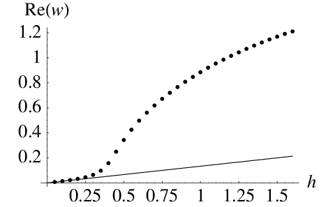 b)
b) 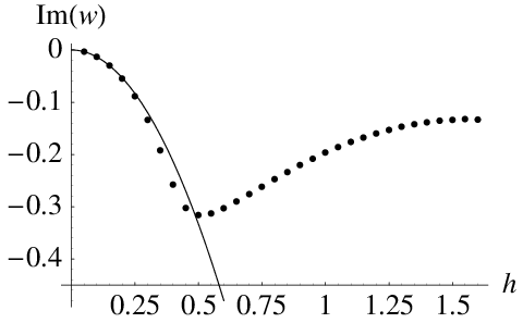
c)  d)
d) 
a)  b)
b) 
In figure 3, we investigate the location of the cyclotron pole in the limit of small and arbitrary . When both and are small, the location of the pole is well approximated by the formulae (9) which were valid precisely when was small. However, as increases, increases as well and the increase eventually takes us out of the regime where (9) is valid.
In figure 4, we look at in the limit of small and arbitrary . In this limit, is always small and the corresponding formulae (9) are expected to be valid always. Indeed, the matching between the numeric and analytic result is remarkably good for all at . This agreement confirms that the combination of limits we considered in the previous section have correctly captured the dependence of the cyclotron pole on arbitrary with small .
7 Discussion
In this paper we have used the AdS/CFT correspondence to study thermoelectric transport in a strongly coupled conformal field theory at finite temperature, electric charge density and background magnetic field. By solving the equations for perturbations about the dual dyonic black hole background, we obtained a combination of analytic and numerical results for the electrical conductivity. We have then shown that this conductivity determines the other thermoelectric transport coefficients of the CFT.
There are two important qualitative features of our results. The first is the existence of relativistic, damped cyclotron resonances due to the background magnetic field. These resonances lead to important features in the conductivity as a function of frequency, as in figure 2. We have explicitly exhibited this resonance as a pole in the complex frequency plane; analytically for small magnetic fields and numerically for general values of the magnetic field. When this pole comes close to the real frequency axis, it can result in semicircle laws for the complexified conductivities as a function of the magnetic field or the frequency.
The second important feature is that electromagnetic duality of the bulk theory acts nontrivially on the transport coefficients of the CFT. In field theory this duality exchanges the values of the background magnetic field and the charge density, and can be thought of as a particle-vortex duality [1, 17]. Under this exchange, we have shown that the complexified conductivity transforms as . Thus the duality constrains the dependence of the conductivity on the magnetic field and charge density. Looking at the conductivity in the complex frequency plane, in figure 1, we see an interesting pattern of poles and zeros that are exchanged under duality. Although exact self-duality is a special feature of CFTs with an Anti-de Sitter dual described by Einstein-Maxwell theory, in the hydrodynamic limit our expressions precisely match generic magnetohydrodynamic (MHD) expectations [16]. Thus we obtain a dual understanding of why relativistic MHD results for the transport coefficients exhibit an interesting and perhaps unexpected duality.
One motivation for our work was to make a connection with the physics of quantum critical phenomena in 2+1 dimensional condensed matter systems. Finite temperature conformal field theories are the appropriate description of such systems when the temperature is the most important scale near the critical point. One example of such critical phenomena is the vicinity of a superfluid-insulator transition in cuprate superconductors. Recent measurements of the Nernst effect in this regime [29] require better theoretical models. The Nernst coefficient measures the transverse voltage arising due to both a thermal gradient and a background magnetic field, and can be computed from and . An MHD calculation of the Nernst coefficient was presented in detail in [16], and some agreement with measurements achieved. Furthermore, the MHD analysis leads to a prediction of a cyclotron resonance which could be observed in the future. In this paper we have derived using the AdS/CFT correspondence all of the formulae that are used in such MHD computations.
Various extensions of our work are possible. For instance, it would be interesting to generalize our MHD formulae to include finite spatial momentum. It would also be of interest to apply our formalism to other asymptotically backgrounds, such as those arising in flux compactifications. Indeed, [30] already studies how Ohm’s law emerges for systems of D-brane probes where the separation of scales between the bulk and D-brane degrees of freedom leads to a finite conductivity at and , in contrast to the results here where translation invariance guarantees the conductivity diverges in this limit. To get a finite conductivity at , in another possible extension of this work, we would need to find a holographic way of adding disorder to our system. Finally, we would like to know if there are physical systems other than those discussed in [16] where relativistic MHD is an appropriate description. So far, we do not see a direct connection between the standard AdS/CFT setups and the (fractional) quantum Hall effect, but any such connection would be fascinating.
Acknowledgments
We would especially like to thank Andreas Karch for many helpful comments and collaboration in the early stages of this project. It is also a pleasure to acknowledge conversations with David Berman, Cliff Burgess, Pavel Kovtun, Markus Müller, Andy O’Bannon, Subir Sachdev, Dam Son, and Larry Yaffe. Both authors acknowledge the hospitality of the Perimeter Institute where part of this work was completed. This research was supported in part by the National Science Foundation under Grant No. PHY05-51164 and in part by the U.S. Department of Energy under Grant No. DE-FG02-96ER40956.
References
- [1] C. P. Herzog, P. Kovtun, S. Sachdev and D. T. Son, “Quantum critical transport, duality, and M-theory,” Phys. Rev. D 75, 085020 (2007) [arXiv:hep-th/0701036].
- [2] J. M. Maldacena, “The large N limit of superconformal field theories and supergravity,” Adv. Theor. Math. Phys. 2, 231 (1998) [Int. J. Theor. Phys. 38, 1113 (1999)] [arXiv:hep-th/9711200].
- [3] S. S. Gubser, I. R. Klebanov and A. M. Polyakov, “Gauge theory correlators from non-critical string theory,” Phys. Lett. B 428, 105 (1998) [arXiv:hep-th/9802109].
- [4] E. Witten, “Anti-de Sitter space and holography,” Adv. Theor. Math. Phys. 2, 253 (1998) [arXiv:hep-th/9802150].
- [5] S. Sachdev, Quantum Phase Transitions, Cambridge University Press, Cambridge (1999).
- [6] S. A. Hartnoll and P. Kovtun, “Hall conductivity from dyonic black holes,” arXiv:0704.1160 [hep-th].
- [7] R. G. Cai and K. S. Soh, “Critical behavior in the rotating D-branes,” Mod. Phys. Lett. A 14, 1895 (1999) [arXiv:hep-th/9812121].
- [8] A. Chamblin, R. Emparan, C. V. Johnson and R. C. Myers, “Charged AdS black holes and catastrophic holography,” Phys. Rev. D 60, 064018 (1999) [arXiv:hep-th/9902170].
- [9] M. Cvetic and S. S. Gubser, “Phases of R-charged black holes, spinning branes and strongly coupled gauge theories,” JHEP 9904, 024 (1999) [arXiv:hep-th/9902195].
- [10] D. T. Son and A. O. Starinets, “Minkowski-space correlators in AdS/CFT correspondence: Recipe and applications,” JHEP 0209, 042 (2002) [arXiv:hep-th/0205051].
- [11] C. P. Herzog and D. T. Son, “Schwinger-Keldysh propagators from AdS/CFT correspondence,” JHEP 0303, 046 (2003) [arXiv:hep-th/0212072].
- [12] C. P. Herzog, “The hydrodynamics of M-theory,” JHEP 0212, 026 (2002) [arXiv:hep-th/0210126].
- [13] C. P. Herzog, “The sound of M-theory,” Phys. Rev. D 68, 024013 (2003) [arXiv:hep-th/0302086].
- [14] O. Saremi, “The viscosity bound conjecture and hydrodynamics of M2-brane theory at finite chemical potential,” JHEP 0610, 083 (2006) [arXiv:hep-th/0601159].
- [15] C. P. Herzog, S. Jeon, L. G. Yaffe, to appear
- [16] S. Hartnoll, P. Kovtun, M. Müller, and S. Sachdev, “Theory of the Nernst effect near quantum phase transitions in condensed matter, and in dyonic black holes,” arXiv:0706.3215 [cond-mat].
- [17] E. Witten, “SL(2,Z) action on three-dimensional conformal field theories with Abelian symmetry,” arXiv:hep-th/0307041.
- [18] R. G. Leigh and A. C. Petkou, “SL(2,Z) action on three-dimensional CFTs and holography,” JHEP 0312, 020 (2003) [arXiv:hep-th/0309177].
- [19] S. de Haro and P. Gao, “Electric - magnetic duality and deformations of three-dimensional CFT’s,” arXiv:hep-th/0701144.
- [20] A. C. Petkou, “Holography, duality and higher-spin theories,” arXiv:hep-th/0410116.
- [21] E. Fradkin and S. Kivelson, “Modular invariance, self-duality and the phase transition between quantum Hall plateaus,” Nucl. Phys. B 474, 543 (1996).
- [22] G. Policastro, D. T. Son and A. O. Starinets, “From AdS/CFT correspondence to hydrodynamics. II: Sound waves,” JHEP 0212, 054 (2002) [arXiv:hep-th/0210220].
- [23] N. R. Cooper, B. I. Halperin, and I. M. Ruzin, “Thermoelectric response of an interacting two-dimensional electron gas in a quantizing magnetic field,” Phys. Rev. B, 55, 2344 (1997).
- [24] D. T. Son and A. O. Starinets, “Hydrodynamics of R-charged black holes,” JHEP 0603, 052 (2006) [arXiv:hep-th/0601157].
- [25] M. Hilke et al. “Semicircle: an exact relation in the Integer and Fractional Quantum Hall Effect,” Europhys. Lett. 46, 776 (1999) [arXiv:cond-mat/9810217].
- [26]
A. M. Dykhne and I. M. Ruzin,
“Theory of the fractional quantum Hall effect: The two-phase model,”
Phys. Rev. B50, 2369 (1994);
I. Ruzin and S. Feng, “Universal Relation between Longitudinal and Transverse Conductivities in Quantum Hall Effect,” Phys. Rev. Lett. 74, 154 (1995). - [27]
C. A. Lütken and G. G. Ross,
“Duality in the Quantum Hall system,”
Phys. Rev. B45, 11837 (1992);
“Delocalization, duality, and scaling in the quantum Hall system,” Phys. Rev. B48, 2500 (1993). - [28] C. P. Burgess, R. Dib and B. P. Dolan, “Derivation of the Semi-circle Law from the Law of Corresponding States,” Phys. Rev. B 62, 15359 (2000) [arXiv:cond-mat/9911476].
- [29] L. Li, J. G. Checkelsky, S. Komiya, Y. Ando, N. P. Ong, “Low-temperature vortex liquid in La2-xSrxCuO4,” Nature Physics 3, 311 (2007).
- [30] A. Karch and A. O’Bannon, “Metallic AdS/CFT,” arXiv:0705.3870 [hep-th].