The essential feature of volume weighted measures is that they reward those regions which expand most rapidly. That is, in a given increment of time, $\Delta t$, the 3-volume of each type of vacuum is increased as a function of its rate of expansion, in some proportionate way. Clearly the way in which time is measured is of primary importance here. For definiteness we will define ‘time’ as being the proper time measured by a congruence of comoving observers. This can be measured in an invariant way in units of the 11-dimensional Planck time, or by equipping each observer with a suitably constructed light clock. Inflation occurs in each vacuum until a tunneling event creates a bubble of new vacuum in the old (or on rare occasions until Minkowski space is reached, if this exists in the theory). The number of points in any particular vacuum that do not eventually undergo a transition to a bubble of new vacuum are a set of measure zero. However, due to the rapid expansion of high-energy vacua, such vanishingly small sets can still come to dominate the evolution of the universe. To make these ideas concrete, we will illustrate this behavior with an example.

Consider a simple landscape of 3 de Sitter vacua, as shown in Figure 1. Here $\kappa_{ij}$ denotes the transition rate from vacuum $i$ to vacuum $j$, and the $H_{i}$ are Hubble constants. We assume that vacuum 1 has a much higher cosmological constant than vacua 2 and 3, so that $H_{1}\gg H_{2,3}$ and $\kappa_{1i}\gg\kappa_{i1},\ \kappa_{23},\ \kappa_{32}$.

If $P_{i}$ is the (unnormalized) probability of finding a given point in the vacuum state $i$, then we can describe this dynamical system through a set of coupled ODEs [10], [11]:

	$\displaystyle\dot{P_{1}}$	$\displaystyle=$	$\displaystyle\kappa_{21}P_{2}+\kappa_{31}P_{3}-(\kappa_{12}+\kappa_{13})P_{1}+3H_{1}P_{1}\ ,$
	$\displaystyle\dot{P_{2}}$	$\displaystyle=$	$\displaystyle\kappa_{12}P_{1}+\kappa_{32}P_{3}-(\kappa_{23}+\kappa_{21})P_{2}+3H_{2}P_{2}\ ,$
	$\displaystyle\dot{P_{2}}$	$\displaystyle=$	$\displaystyle\kappa_{13}P_{1}+\kappa_{23}P_{2}-(\kappa_{32}+\kappa_{31})P_{3}+3H_{3}P_{3}.$

As long as $H_{1}\gg\kappa_{ij}$ for all $i$, $j$ (i.e. the highest energy vacuum expands much faster than it decays), the first of these equations becomes

$$\dot{P_{1}}\simeq 3H_{1}P_{1}\qquad\qquad\Rightarrow\qquad\qquad P_{1}\propto e^{-3H_{1}t}.$$

The terms dominating the RHS of the second two equations are then those which are proportional to $P_{1}$, as $t\rightarrow\infty$. These equations are solved by

$$\frac{P_{i}}{P_{1}}\simeq\frac{\kappa_{1i}}{3H_{1}}\ll 1\qquad\qquad\text{or}\qquad\qquad\frac{P_{i}}{P_{j}}\simeq\frac{\kappa_{1i}}{\kappa_{1j}}.$$

This confirms that the probability of finding a point in any particular vacuum is proportional to its rate of decay from the highest energy (fastest-growing) vacuum. Essentially, the most rapidly expanding vacuum sources all of the others – it is easier to make the lower vacua by expanding in vacuum 1 and then decaying down, than it is to do so by simply expanding with the smaller Hubble constant of the lower vacua.

These results readily generalize to more complicated systems. First, consider a landscape in which the highest energy vacuum can decay to all other vacua. In this case we have

$$\frac{P_{i}}{P_{h}}\simeq\frac{\kappa_{hi}}{3H_{h}}\ll 1\qquad\qquad\text{or}\qquad\qquad\frac{P_{i}}{P_{j}}\simeq\frac{\kappa_{hi}}{\kappa_{hj}},$$

(1)

where $h$ labels the highest energy vacuum. Now consider a landscape in which there exist vacua that cannot be created from direct decays from the highest energy state. In this case the probability of finding a point in the vacuum state $j$ is

$$\frac{P_{j}}{P_{h}}=\sum_{\stackrel{{\scriptstyle all}}{{paths}}}\frac{\kappa_{ha}}{3H_{h}}\times\frac{\kappa_{ab}}{3H_{h}}\times\frac{\kappa_{bc}}{3H_{h}}\times...\times\frac{\kappa_{ij}}{3H_{h}}\ll 1.$$

(2)

The chain of $\kappa_{ij}/3H_{h}$ gives the probability of starting in the state $h$ and finishing in $j$, following some series of decays through the vacua $a$, $b$, $c...$. To obtain the total probability of finding a point in the vacuum $j$ it is then necessary to sum over all possible paths. Clearly some paths will provide more of a contribution than others to this sum. In fact, as long as $\kappa_{ij}\ll H_{h}$, only the shortest decay chains will give a significant contribution. Every chain with additional, unnecessary, intermediary vacua will be suppressed by factors of $\kappa_{ij}/3H_{h}\ll 1$. However, if $\kappa_{ij}\sim 3H_{h}$ then the products of decay are no longer suppressed. In this case the progeny of decaying vacua will be as equally abundant as the vacua from which they decayed. Rapid transitions of this type will not contribute suppressing factors to the decay chains mentioned above.

We will consider here the Bousso-Polchinski (BP) landscape of M-Theory [2]. This model has the advantages of being relatively simple and, most importantly for our purposes, having known expressions for the transition rates.

The BP landscape consists of a discrete set of vacua, each with a different effective cosmological constant given by

$$\Lambda=-\Lambda_{0}+\frac{1}{2}\sum_{i=1}^{J}q_{i}^{2}n_{i}^{2},$$

(3)

where $J$ is the number of fluxes, $q_{i}$ the charge associated with each of them and $n_{i}$ the number of units of a particular flux. The discreteness of the $n_{i}$ arises from the quantization of four-form fluxes in M-theory compactifications, and their multiplicity from the geometry of the M-theory compactification – each non-trivial three-cycle giving rise to a different four-form flux. The number of such cycles is generically quite large. This multiplicity allows a much finer spacing of $\Lambda$ than that given by a single flux alone, which typically has a charge only a few orders of magnitude below the Planck scale [2].

From equation (3) it is clear that for a given choice of $\Lambda$, the fluxes are constrained to lie on a sphere in flux space, of radius $\sqrt{2(\Lambda+\Lambda_{0})}$. Taking $0\leqslant\Lambda\lesssim 10^{-120}$ (in 4D Planck units) we obtain a thin shell of radius $\sim\sqrt{2\Lambda_{0}}$, which corresponds to the set of vacua in the BP landscape which have an anthropically acceptable cosmological constant (see below).

Transitions in this landscape occur via the nucleation of branes. The transition rates, including gravitational effects, are given by [12]

$$\kappa_{ij}=A_{ij}e^{-B_{ij}}\ .$$

(4)

The $A_{ij}$ can be approximated by $A_{ij}\sim 1$ (any effect they have will be exponentially unimportant). Now let us consider the nucleation of bubbles which change the flux through some particular cycle by one unit, from $n_{i}$ to $n_{i}-1$, such that

$$|\Delta\Lambda_{i}|=(n_{i}-1/2)q_{i}^{2}\ .$$

The tunneling rate is then given as the product of its value in flat space, times some gravitational correction, as [13]

$$B_{i\downarrow}=B^{\textrm{flatspace}}_{i\downarrow}r(x,y),$$

(5)

where the gravitational correction factor is

$$r(x,y)=\frac{2[(1+xy)-(1+2xy+x^{2})^{1/2}]}{x^{2}(y^{2}-1)(1+2xy+x^{2})^{1/2}},$$

(6)

and the flat space rate is [14]

$$B^{\textrm{flat-space}}_{i\downarrow}=\frac{27\pi^{2}}{8}\frac{1}{(n_{i}-1/2)^{3}q_{i}^{2}}.$$

(7)

The dimensionless parameters in $r(x,y)$ are given by

$$x\equiv\frac{3q_{i}^{2}}{8|\Delta\Lambda_{i}|}=\frac{3}{8(n_{i}-1/2)}\qquad\qquad\text{and}\qquad\qquad y\equiv\frac{2\Lambda}{|\Delta\Lambda_{i}|}-1\ .$$

(8)

For our purposes $n_{i}$ will always be $\gg 1$, so that $x\simeq 3/8n\ll 1$. The variable $y$ has a clear interpretation as the energy-level of the parent vacuum. At high energies $\Lambda_{i}\gg|\Delta\Lambda_{i}|$, so that $y\gg 1$. Conversely, at the lowest energies $\Lambda_{i}\sim|\Delta\Lambda_{i}|$, so that $y\sim 1$. The combination $xy$ can be interpreted as a measure of distance from the axes of the flux space. Consider the surface defined by $xy=3/8$, we then have

$$xy\simeq\frac{3}{8n_{i}}\frac{2\Lambda_{i}}{|\Delta\Lambda_{ij}|}\simeq\frac{3}{4}\frac{\Lambda}{n_{i}^{2}q_{i}^{2}}\simeq\frac{3}{8}\qquad\Rightarrow\qquad\sum_{k\neq i}n_{k}^{2}q_{k}^{2}\simeq 2\Lambda_{0}.$$

The LHS of this second equation is the perpendicular distance (squared) away from the axis corresponding to the direction in which the transition is occurring. The RHS is the radius (squared) of the anthropic shell. Therefore when $xy\lesssim 3/8$ the transition is occurring in a cylinder around this axis, of the same cross-sectional area as the anthropic shell. When $xy\gg 3/8$ the transition is occurring well away from the axis.

Useful estimates of tunneling rates can be found in a number of different regimes [7]. Firstly, at high energies far from the axis, when $y\gg 1$ and $xy\gg 1$, it can be seen that

$$\qquad r(x,y)\simeq\sqrt{2}(xy)^{-3/2}\ll 1.$$

(9)

The tunneling rate (5) is then given by

$$\kappa_{ij}\simeq\textrm{Exp}\left[-\frac{3\sqrt{6}\pi^{2}q_{i}}{\Lambda_{i}^{3/2}}\right].$$

(10)

This expression is independent of $n_{i}$. Alternatively, closer to the axis, when $y\gg 1$ and $xy\ll 1$, we obtain the Padé approximant

$$r(x,y)\simeq\frac{1-xy}{1+xy}.$$

(11)

This approaches the flat space limit as $xy\rightarrow 0$:

$$\kappa_{ij}\sim\textrm{Exp}\left[-\frac{27\pi^{2}}{8}\frac{1}{n_{i}^{3}q_{i}^{2}}\right].$$

(12)

Another regime of interest is at low energy, when $y\sim 1$: that of the final transition, down into the anthropic shell. In this limit [12]

$$r(x,y)\simeq(1+x^{2})^{-2}=\frac{(n_{i}-1/2)^{2}}{(n_{i}-1/8)^{2}}\simeq 1,$$

such that the gravitational correction is vanishingly small. As long as this condition is met, we can then approximate the tunneling rate down into the anthropic shell by equation (12).

The flat space tunneling rate is shown graphically, as a function of angular coordinates, in figure 2.

It can be seen that $\kappa_{ij}$ is significantly larger near the axes of this space, even in these few dimensions. In more dimensions, the contrast between maximum and minimum is increased. This expression for $\kappa_{ij}$ will be used below to show that even a single transition (the last one) can produce considerable clustering of probability around the axes of the flux space. As the radius of the sphere being considered (and hence the energy level) is increased, gravitational corrections must increasingly be taken into consideration. The effect of gravity is to reduce the contrast between maxima and minima, smoothing the distribution of $\kappa_{ij}$ and producing a plot that looks more like a sphere.

As well as nucleating branes of single charge, one may also wish to consider the possibility of nucleating stacks of branes simultaneously. A study of such events has been carried out by Garriga and Megevand [15]. In this work it is concluded that the instantons for nucleating stacks of branes may well not exist, but if they do then the tunneling rates for such events will be approximately given by $B^{(k)}_{ij}\simeq kB_{ij}$, where $k$ is the number of branes in the stack and $B^{(k)}$ is the exponent of the tunneling rate for nucleating the stack. This formula was found in the limit that the bubble wall is much less than the Hubble rate of the parent vacuum, in which case the thin-wall approximation can be used. When a sufficiently large stack is nucleated (again, if this is possible), then the thin wall approximation is violated and the bound on the minimum possible tunneling rate [16] is saturated. In this limit, the exponent of the tunneling rate was found to be $B^{(k)}_{ij}\simeq\frac{8\pi^{2}}{\Lambda_{i}}$. This rate is independent of the everything except the energy of the parent vacuum, and so once it is met all unlikely tunneling events proceed with this minimum probability, if instantons for these transitions exist at all.

The possibility of nucleating stacks of branes significantly alters the dynamics of inflation, if it is allowed to occur. We consider it beyond the scope of the present study to perform a detailed analysis of this phenomenon here. Instead, we will first proceed using the standard lore of allowing only transitions between nearest neighbors in the BP landscape. After analyzing this situation we will then reflect on how nucleating multiple branes simultaneously will change this picture. We leave it to future studies to determine how likely these events really are.

In volume weighted measures of inflation the majority of the 3-volume of the universe, and the majority of new bubbles formed, are at very high energies. However, no observers can exist in these vacua. Firstly, the famous anthropic bound on the cosmological constant tells us that anthropically acceptable vacua must lie within the range $0\lesssim\Lambda\lesssim 10^{-120}$ in order for structure to be able to form [17] (we neglect the possibility of small negative cosmological constant [18], for simplicity). Secondly, these high energy vacua decay far too quickly for structure to form. If we are interested in the likely locations in the landscape for observers to find themselves we should therefore not ask simply what are the most likely vacua, but instead what are the most likely vacua that (a) have a suitably low cosmological constant, and (b) are suitably long-lived⁵⁵ 5 There are a number of other anthropic bounds that should also be applied from, for example, the fine structure constant and Newton’s constant. For simplicity, and due to the limited nature of our model, we will not consider all of these bounds here..

In order to consider the distribution of probability on a sphere it is useful to determine the moments

$$\langle f^{2}\rangle\equiv\int f^{2}\kappa_{T}d\Omega$$

(20)

where $f=f(x_{i},z)$ is any function of $x_{i}$ and $z$ on the sphere, and $d\Omega$ is the surface element of a hypersphere. This expression takes into account not only the effect of the transition rate $\kappa_{T}$, but also the effect of increasing surface area away from the axes.

We can consider the penultimate sphere as being divided into $2J$ symmetric sectors, each centered around one of the $2J$ axes of the space. Each of these sectors corresponds to the region $\sigma$ on the surface of the penultimate sphere which is closest to the axis about which it is centered. $z$ is then given, in each respective region, as the corresponding value of the Cartesian coordinate along its central axis, and the whole sphere is built up by evaluating $\langle n^{2}\rangle$ in any one of the regions and multiplying it by $2J$. The integral that we are now required to evaluate is

$$\langle f^{2}\rangle=\int_{0}^{1}dz\prod_{i}^{J-1}\int_{-z}^{z}dx_{i}f^{2}e^{-12/z^{2}}\delta\left(\sum_{i}^{J-1}x_{i}^{2}+z^{2}-1\right),$$

(21)

where we have taken $\Lambda_{0}=1/2$. The Cartesian coordinates $x_{i}$ correspond to all of those directions which are orthonormal to the central axis $z$. The limits of integration, $-z$ and $z$, then pick out the sector discussed above. Included in the integrand is a delta function intended to select the surface at $\sim\sqrt{2\Lambda_{0}}=1$, which corresponds to the anthropic shell. Here $\langle f^{2}\rangle$ is being evaluated in any one of the $2J$ symmetric regions. We will be interested in the choices $f=z$ and $f=x$, where $x$ is any Cartesian coordinate orthonormal to $z$. The moments $\langle z^{2}\rangle$ and $\langle x^{2}\rangle$ then give us the expectation values of these quantities, and their ratio gives us a measure of the peaking of probability on the anthropic sphere due to tunneling down from high energy to the penultimate sphere before the anthropic one.

In appendix B we find that the expectation values for $\langle z^{2}\rangle$ and $\langle x^{2}\rangle$ can be given in terms of one-dimensional integrals as

$$\langle z^{2}\rangle=\frac{2}{\Gamma(\frac{J+2}{2})}\int_{0}^{\infty}dyy^{2}\left[\frac{\sqrt{\pi}y}{\sqrt{12+y^{2}}}E(\sqrt{12+y^{2}})\right]^{J-1}e^{-(12+y^{2})}$$

(22)

and

	$\displaystyle\langle x^{2}\rangle$	$\displaystyle=\frac{2}{\Gamma(\frac{J+2}{2})}\int_{0}^{\infty}dyy^{2}\left(\frac{1}{2(12+y^{2})}-\frac{e^{-(12+y^{2})}}{\sqrt{\pi}\sqrt{12+y^{2}}E(\sqrt{12+y^{2}})}\right)$
		$\displaystyle\hskip 200.0pt\times\left[\frac{\sqrt{\pi}y}{\sqrt{12+y^{2}}}E(\sqrt{12+y^{2}})\right]^{J-1}e^{-(12+y^{2})}.$		(23)

Here the function $E(p)$ is the integral of a Gaussian distribution, or error function, given by $2\pi^{-1/2}\int_{0}^{p}e^{-q^{2}}dq$.

The measure of peaking that we are interested in is given by the ratio of these two expressions, $\langle z^{2}\rangle/\langle x^{2}\rangle$. This is shown graphically in figure 4. It can be seen from this plot that the peaking produced by tunneling down to the penultimate sphere is extremely sharp, and increases with the dimensionality of the flux space.

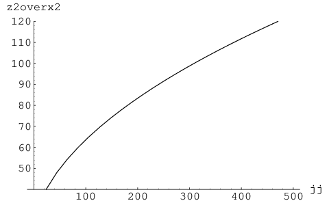
A flat distribution of probability would produce the result $\langle z^{2}\rangle/\langle x^{2}\rangle=1$. The large values of this quantity here show that there exists a strong peak in probability on the anthropic shell.

We are now in a good position to investigate approximations that will make these quantities more transparent. A particularly useful simplification is to extend the domain of integration of equation (21), to make it independent of $z$. If we were to allow the limits of integration for the coordinates $x_{i}$ to run from $-1$ to $1$, instead of $-z$ to $z$, then this would allow us to transform to a hyper-cylindrical coordinate system in which $J-1$ of the dimensions could be integrated over in a straightforward fashion. This would leave a simple one-dimensional integral that can be solved by saddle point approximation. We will call this the single peak approximation, as we will be integrating over a larger region that should contain several peaks of probability; we will, however, ignore all but the single central peak of the initial region and show that this is a good approximation to integrating over the correct domain, as in (21). The reason why this is a plausible approximation to consider is that the rate of transitions (19) can be seen to become very small at low $z$. The extra region being integrated over in the single peak approximation is all at low $z$, and so it is a reasonable proposition to ask if integrating over such an extended domain yields similar results to integrating over the actual domain of interest. We will argue that it does.

The single peak approximation yields the results

	$\displaystyle\langle\bar{z}^{2}\rangle$	$\displaystyle=\frac{2}{\Gamma(\frac{J+2}{2})}\int_{0}^{\infty}dz\prod_{i}^{J-1}\int_{-\infty}^{\infty}dx_{i}z^{2}e^{-(\sum_{i}x_{i}^{2}+z^{2})(1+12z^{-2})}$
		$\displaystyle=\frac{2}{\Gamma(\frac{J+2}{2})}\int_{0}^{\infty}dzz^{2}\left[\frac{\sqrt{\pi}z}{\sqrt{12+z^{2}}}\right]^{J-1}e^{-(12+z^{2})},$		(24)

which can be compared to equation (22), and

	$\displaystyle\langle\bar{x}^{2}\rangle$	$\displaystyle=\frac{2}{\Gamma(\frac{J+2}{2})}\int_{0}^{\infty}dz\prod_{i}^{J-1}\int_{-\infty}^{\infty}dx_{i}x^{2}e^{-(\sum_{i}x_{i}^{2}+z^{2})(1+12z^{-2})}$
		$\displaystyle=\frac{2}{\Gamma(\frac{J+2}{2})}\int_{0}^{\infty}dz\frac{z^{2}}{2(12+z^{2})}\left[\frac{\sqrt{\pi}z}{\sqrt{12+z^{2}}}E(\sqrt{12+z^{2}})\right]^{J-1}e^{-(12+z^{2})},$		(25)

which can be compared to equation (23). We denote quantities evaluated in the single peak approximation by an over-bar. The fractional error of considering this approximation can then be written as

$$\delta\equiv\frac{\langle z^{2}\rangle/\langle x^{2}\rangle-\langle\bar{z}^{2}\rangle/\langle\bar{x}^{2}\rangle}{\langle z^{2}\rangle/\langle x^{2}\rangle}.$$

(26)

This quantity is vanishingly small for all $J$, showing that the single peak approximation is very good.

Using the single peak approximation we will now find analytic expressions for these moments. Recall the tunneling rate is given by

$$\kappa_{T}\sim\textrm{Exp}\left[-\frac{12}{z^{2}}\right]=\textrm{Exp}\left[-\frac{K}{z^{2}}\right],$$

(27)

where $K=12$, and to be concise we have replaced $z_{0}$ with $z$. The normalization of the probability distribution is then

$$N=\int\kappa d\Omega=2J\int_{0}^{1}dz\prod_{i}^{J-1}\int_{-1}^{1}dx_{i}e^{-K/z^{2}}\delta\left(\sum_{j}^{J-1}x_{i}^{2}+z^{2}-1\right)\ .$$

(28)

In the single peak approximation, the limits on the $x_{i}$ integrals are replaced with -1 and 1. Changing coordinates from Cartesian to hyper-cylindrical, and defining $r^{2}=\sum_{i}^{J-1}x_{i}^{2}$, we can rewrite $N$ as

$$N=2JV_{J-2}\int_{0}^{1}dz\int_{0}^{1}drr^{J-2}e^{-K/z^{2}}\delta(r^{2}+z^{2}-1)\ ,$$

(29)

where $V_{J-2}$ is the volume of a $(J-2)$-sphere. Eliminating the delta function with the $r$-integral leaves us with an integral over $z$:

$$N=2JV_{J-2}\int_{0}^{1}dz(1-z^{2})^{\frac{J-3}{2}}e^{-K/z^{2}}\sim 2JV_{J-2}\int_{0}^{1}dze^{-\left(K/z^{2}-\frac{J}{2}\textrm{ln}(1-z^{2})\right)}\ .$$

(30)

This integral can be approximated by a saddle point, which is at

$$z^{2}=\frac{K}{J}\left(-1+\sqrt{1+\frac{2J}{K}}\right)\sim\sqrt{\frac{2K}{J}}=\left(\frac{24}{J}\right)^{1/4}.$$

(31)

At first glance it may seem that this result is in contradiction with the validity of the single peak approximation. After all, $z$ is small for any reasonable $J$ ($\tilde{C}\lesssim 1$) and therefore $r$ is close to 1. However, although $z$ is small, a typical $x_{i}$ ($\sim 1/\sqrt{J}$) is much smaller and so the peak in the distribution on the sphere is, in general, closer to the $z$-axis than to any of the other $x_{i}$ axes. This issue is discussed in more detail in section 6.

We can similarly calculate the expectation values of powers of the fluxes:

$$\langle z^{k}\rangle=\frac{1}{N}V_{J-2}\int_{0}^{1}dzz^{k}(1-z^{2})^{\frac{J-3}{2}}e^{-K/z^{2}}\sim\frac{1}{N}V_{J-2}\int_{0}^{1}dze^{-\left(K/z^{2}-\frac{J}{2}\textrm{ln}(1-z^{2})-k\,\textrm{ln}(z)\right)}\ .$$

(32)

This should be normalized using the $N$ calculated above. The integrand is again extremized at $z\sim\left(\frac{2K}{J}\right)^{1/4}$ (with an $O((2K/J)^{1/4}(k/J))$ correction). Substituting this back into the integral above, and evaluating the saddle point, gives us

$$\langle z^{k}\rangle\sim\left(\frac{2K}{J}\right)^{k/4}=\left(\frac{24}{J}\right)^{k/4}\ .$$

(33)

Here the normalization $N$ cancels the exponential, the remaining integral and various other numerical factors. In a flat measure the same expectation value is given by

$$\langle z^{k}\rangle_{\textrm{flat}}=\frac{V_{J-2}}{N_{\textrm{flat}}}\int_{0}^{\infty}dr(1-r^{2})^{(k-1)/2}r^{J-2}\ .$$

(34)

The scaling with $J$ can again be obtained, and is now found to be

$$\langle z^{k}\rangle_{\textrm{flat}}\sim\left(\frac{1}{J}\right)^{k/2}.$$

(35)

Symmetry considerations then give the expected values of the remaining fluxes as

$$\langle x_{i}^{k}\rangle\sim\frac{1}{J^{k/2}},$$

(36)

and a typical flux vector can be estimated as

$$q\vec{n}\sim\left(\left(\frac{2K}{J}\right)^{1/4}\ ,\ \frac{1}{J^{1/2}}\ ,\ \ldots\ ,\ \frac{1}{J^{1/2}}\right)\ ,$$

(37)

which, for $J=500$ and $q=10^{-2}$, is

$$\vec{n}\sim\left(45\ ,\ 4.5\ ,\ \ldots\ ,\ 4.5\right)\ .$$

(38)

Therefore, the most likely vacua produced by tunneling down from high energies to the penultimate sphere are those with one flux approximately ten times as large as the others. The spread of probability about this most likely point will be addressed in section 6. Here we have assumed that all charges are the same. Allowing different charges will produce sharper peaking near the axes associated with smaller $q$.

Working in the single peak approximation we can use saddle points methods, as before, to estimate the level of peaking from the final transition. We begin with the integral

$$N=\int\kappa d\Omega=2J\int_{0}^{1}dz\prod_{i}^{J-1}\int_{-z}^{z}dx_{i}e^{-\tilde{C}/z^{3}}\delta\left(\sum_{j}^{J-1}x_{i}^{2}+z^{2}-1\right)\ ,$$

(41)

which has its integrand extremized at

$$z\sim\left(\frac{3\tilde{C}}{J-2}\right)^{1/5}\ .$$

(42)

Again, the integral has most of it’s support relatively close to the $z$ axis, consistent with the single peak approximation.

Once again we can calculate the expected fluxes from the integral

$$\langle z^{k}\rangle=\frac{V_{J-2}}{N}\int_{0}^{\infty}dr(1-r^{2})^{(k-1)/2}r^{J-2}e^{-\tilde{C}/(1-r^{2})^{3/2}}\ ,$$

(43)

which has its saddle point given by 42 (with an $O(\epsilon k^{2}/J)$ correction), and thus

$$\langle z^{k}\rangle\sim\left(\frac{3\tilde{C}}{J-2}\right)^{k/5}\sim\left(\frac{1}{J}\right)^{k/5}.$$

(44)

This allows us to write a typical vector as

$$q\vec{n}\sim\left(\frac{1}{J^{1/5}}\ ,\ \frac{1}{J^{1/2}}\ ,\ \ldots\ ,\ \frac{1}{J^{1/2}}\right)\ .$$

(45)

For $J=500$ and $q=10^{-2}$ we should then typically expect to find one set of preferred fluxes to be over 6 times greater than the others:

$$\vec{n}\sim\left(29\ ,\ 4.5\ ,\ \ldots\ ,\ 4.5\right)\ .$$

(46)

These saddle point approximations are shown graphically in figure 5, where they are compared to direct numerical integrations.

The peaking found here is clearly less than that found in the previous section, and we will now show that its effects are negligible in comparison. The total tunneling rate from combining (19) and (39) is

$$\kappa\simeq\text{Exp}\left[-\frac{12}{z_{0}^{2}}-\frac{0.3}{z_{0}^{3}}\right].$$

It can be seen that the second term in this expression only becomes important at about $z_{0}\sim 1/40$. Before this the first term dominates, and the expression is well approximated by (19). This critical value of $z_{0}$ can be seen to be an order of magnitude smaller than the location of the saddle points involved in either this, or the previous, section. As both of the saddle-points are located comfortably in the region where (19) is a good approximation to the total tunneling rate, we consider the effects of this last transition to be negligible in comparison to those considered in the last section. This is supported by the relatively mild peaking found above.

We will now refine our assertion that the measure on the anthropic sphere is sharply peaked, and give a demonstration of the level of this peaking. We begin our argument by considering the tunneling down from high to low energies, as discussed in section 4. We do this by noting that near the peak the distribution is Gaussian, and then calculating the standard deviation.

We begin with the integral (30) and note that the saddle point approximation gives us not only the position of the peak, but also the width. The leading contribution to this is found to be

$$\sigma^{2}\sim\frac{1}{8J}.$$

(47)

Now consider the flat probability distribution on the sphere, where

$$N_{\textrm{flat}}=V_{J-2}\int dz(1-z^{2})^{(J-3)/2},$$

(48)

at $z\ll 1$ this can be approximated by

$$N_{\textrm{flat}}\sim V_{J-2}\int dz\textrm{Exp}[-Jz^{2}/2]\ .$$

(49)

Evidentally the integrand falls at least exponentially for $z\gtrsim J^{-1}$, and grows rapidly above $z\lesssim J^{-1}$. Roughly speaking, this means that whilst the probability distribution integral has most of its support around $z^{4}=24/J$, most of the volume of the sphere lies further out, around $z=1/J$. This is represented graphically in figure 6, where it is clear that the overlap between the probability peak and the volume peak decreases as $J$ is increased – i.e. more and more of the volume of the anthropically acceptable parts of the multiverse come from smaller and smaller fractions of the surface of the anthropic sphere.

We can then estimate what fraction, $f$, of the sphere is covered by $m\sigma$ of the probability distribution, by evaluating the volume integral (49) between the limits $\langle z\rangle-m\sigma$ and $\langle z\rangle+m\sigma$:

$$f=2J\frac{V_{J-2}}{V_{J-1}}\int_{\langle z\rangle-m(8J)^{-1/2}}^{\langle z\rangle+m(8J)^{-1/2}}dz\textrm{Exp}[-Jz^{2}/2]\ .$$

(50)

We can bound this integral by multiplying the maximum of volume integrand (which is at $z=(2K)^{1/4}/J^{1/4}+m(8J)^{-1/2}$) by the total range of the integral ($2m\sigma$). The leading contribution is given by

$$f\sim 2J\frac{V_{J-2}}{V_{J-1}}\frac{2m}{J}e^{-Jz^{2}/2}\sim 2J\frac{V_{J-2}}{V_{J-1}}\frac{2m}{J}e^{-\frac{(24J)^{1/2}}{2}}\sim 4m\sqrt{J}e^{-\frac{(24J)^{1/2}}{2}}.$$

(51)

For $J=500$ we find that 99.9999% of the volume of the universe (5 standard deviations) covers $\sim 10^{-23}$ of the anthropic region.

This argument can be repeated for the final transition down onto the anthropic sphere, discussed in section 5. Here the fraction of vacua on the anthropic sphere within $m\sigma$ of the peak is

$$f\sim 2J\frac{V_{J-2}}{V_{J-1}}\frac{2m}{J^{7/10}}e^{-\frac{J^{3/5}}{2}}\sim 4mJ^{4/5}e^{-\frac{J^{3/5}}{2}},$$

(52)

where $\sigma\sim J^{-7/10}$. For $J=500$ we then find that 99.9999% of the volume covers only $\sim 10^{-6}$ of the anthropic sphere. Evidentally, this is considerably less than that due to tunneling down from higher energies.

In the preceding sections we have found the most probable vacua that have a cosmological constant in the anthropically acceptable range $0\lesssim\Lambda\lesssim 10^{-120}$. However, for observers to appear we require not only an anthropically acceptable value of $\Lambda$, but also a vacuum that is long enough lived for life to evolve. In section 2.3 this was taken to be $\sim 10$ Gyr. The vacua located at the peaks of probability (found in the previous sections) do not satisfy the bound $\tau>10$ Gyr, and so are unlikely to be stable enough for observers of our type to occur. If we wish to determine the probability of vacua that have both an acceptably small $\Lambda$, and an acceptably large life-time, then we must calculate probabilities only up to the boundary at which $\tau\simeq 10Gyr$. Using our knowledge that there exists a sharp peak of probability outside of this region, we should expect to find a selection pressure pushing against the anthropic life-time barrier (so that vacua closer to the peak are favored). Here we will investigate how strong this selection pressure is, and use it to make a prediction for the half-life of acceptable vacua.

In order to establish the extent to which vacua near the life-time boundary are favored we will consider a thin region next to it. The life-time boundary is at a constant value of $z$, and we will label it by $z_{1}$. The thin region we are considering next to this boundary will extend down to a constant $z=z_{2}$, where $z_{2}<z_{1}$. The volume contained within this region can be approximated by

$$\Delta V\simeq V_{J-2}\int_{z_{2}}^{z_{1}}e^{-\frac{J}{2}z^{2}}dz,$$

(53)

where $V_{J-2}$ is the volume of a $(J-2)$-sphere. The probability of finding a vacuum in this region can then be estimated using the formula (19), and by integrating over the thin band:

$$\Delta P\simeq\int_{z_{2}}^{z_{1}}\kappa_{T}d\Omega\simeq\int_{z_{2}}^{z_{1}}e^{-\frac{J}{2}z^{2}-\frac{12}{z^{2}}}dz.$$

(54)

These integrals can be performed numerically, the results of which are shown in figure 7. Here we have normalized $\Delta P$ so that $\Delta P/P\rightarrow 1$ as $z_{2}\rightarrow 0$. The volume $\Delta V$ is presented as a fraction of the volume of the unit sphere.

It can be seen from the figure that the probability is pressed up against the boundary, within a fractional volume of $\sim 0.001$.

In order to determine the typical distance of an anthropically acceptable vacuum from this boundary we will find the width of strip that is required for half of the probability to be within it, and half outside of it: The half-life of the distribution. The value of $z_{2}$ for such a band is $\sim 0.9995z_{1}$. The life-time of vacua at this value of $z$ is $\sim 12.2$ Gyr. Given the model we have been investigating, with the parameters chosen and assumptions made, we should therefore expect a typical anthropically acceptable vacuum to decay after about $2.2$ billion years from the moment when the first observers appear (at $10$Gyr).

One may have initially suspected that the exponential pressure up against the boundary should cause decay of vacua after a very short time. However, the exponential sensitivity of life-time on $z$ counters this pressure, and results in vacua being reasonably long lived.

References

- [1] For a review see M. Douglas and S. Kachru, “Flux Compactification,” [arXiv:hep-th/0610102].
- [2] R. Bousso and J. Polchinski, “Quantization of Four-Form Fluxes and Dynamical Neutralisation of the Cosmological Constant,” JHEP 0006, 006 (2000) [arXiv:hep-th/0004134].
- [3] T. Clifton, A. Linde and N. Sivanandam, “Islands in the Landscape,” JHEP 0702, 024 (2007) [arXiv:hep-th/0701083].
- [4] A. Linde, “Eternally Existing Self-Reproducing Chaotic Inflationary Universe,” Phys. Lett. B175, 395 (1986).
- [5] A. Linde, “Towards a Gauge Invariant Volume-Weighted Probability Measure for Eternal Inflation,” [arXiv:0705.1160].
- [6] J. Garriga, D. Schwartz-Perlov, A. Vilenkin and S. Winitzki, “Probabilities in the Inflationary Multiverse,” JCAP 0601, 017 (2006) [arXiv:hep-th/0509184].
- [7] D. Schwartz-Perlov and A. Vilenkin, “Probabilities in the Bousso-Polchinski Multiverse,” JCAP 0606, 010 (2006) [arXiv:hep-th/0601162].
- [8] R. Bousso, “Holographic Probabilities in Eternal Inflation,” Phys. Rev. Lett. 97, 191302 (2006) [arXiv:hep-th/0605263].
- [9] R. Bousso and I.-S. Yang, “Landscape Predictions from Cosmological Vacuum Selection,” [arXiv:hep-th/0703206].
- [10] J. Garriga and A. Vilenkin, “Recycling Universe,” Phys. Rev. D 57, 2230 (1998) [arXiv:astro-ph/9707292].
- [11] A. Linde, “Sinks in the Landscape, Boltzmann Brains, and the Cosmological Constant Problem,” JCAP 0701, 022 (2007) [arXiv:hep-th/0611043].
- [12] S. Coleman and F. De Luccia, “Gravitational Effects on and of Vacuum Decay,” Phys. Rev. D 21, 3305 (1980).
- [13] S. Parke, “Gravity and the Decay of False Vacuum,” Phys. Lett. 121B, 313 (1983).
- [14] J. Brown and C. Teitelboim, “Dynamical Neutralization of the Cosmological Constant,” Phys. Lett B195, 177 (1987).
- [15] J. Garriga and A. Megevand, “Coincident Brane Nucleation and Neutralisation of ,” Phys. Rev. D 69, 083510 (2004) [arXiv:hep-th/0310211].
- [16] S. Kachru, R. Kallosh, A. Linde and S. Trivedi, “De Sitter Vacua in String Theory,” Phys. Rev. D 68, 046005 (2003) [arXiv:hep-th/0301240].
- [17] A. Linde, “The Inflationary Universe,” Rept. Prog. Phys. 47, 925 (1984), T. Banks, “T C P, Quantum Gravity, the Cosmological Constant and All That..,” Nucl. Phys. B 249, 332 (1985), S. Weinberg, “Anthropic Bound on the Cosmological Constant,” Phys. Rev. Lett. 59, 2607 (1987).
- [18] A. Linde, “Inflation and Quantum Cosmology,” Print-86-0888 (June 1986), in 300 Years of Gravitation, ed. by S. Hawking and W. Israel, Cambridge University Press, Cambridge (1987).
- [19] K. Olum and D. Schwartz-Perlov, “Anthropic Prediction in a Large Toy Landscape,” [arXiv:0702.2562].
- [20] R. Bousso, R. Harnik, G. Kribs and G. Perez, “Predicting the Cosmological Constant from the Causal Entropic Principle,” [arXiv:hep-th/0702115].