Collider Phenomenology of Unparticle Physics

It was demonstrated in georgi1 that scale invariance can be used to fix the two-point functions of the unparticle operators. Let us consider a two-point function for a scalar unparticle operator $O_{\cal U}$

where $\rho_{\cal U}(P^{2})$ is the spectral density and is formally given by

Inverse Fourier transformation gives

where $\alpha$ is an index to be determined based on scale invariance and $A_{d_{\cal U}}$ is a normalization factor also required to be fixed. Under a scale transformation $x\to s\,x$ and $O_{\cal U}(sx)\to s^{-d_{\cal U}}O_{\cal U}(x)$, we have

Requiring scale invariance implies $\alpha=d_{\cal U}-2$, since the step functions are invariant. Therefore, we obtain

where $A_{d_{\cal U}}$ is normalized to interpolate the $d_{\cal U}$-body phase space of massless particle georgi1. The phase space factor for $n$ massless particle with $(p_{1}+p_{2}+\cdots+p_{n})^{2}=s^{2}$ and $p_{i}^{2}=0$ can be written as

which for the first few $n$’s are $A_{n\to 1}\to 2\pi(n-1)$, $A_{2}={1\over 8\pi}$ and $A_{3}={1\over 256\pi^{3}}$, etc. Based on the similar scale dependence, the unparticle spectral density is identified with the phase space of $d_{\cal U}$-body massless particle in a convention advocated in georgi1: $d_{\cal U}\to n$ and $A_{n}\to A_{d_{\cal U}}$. So the factor $A_{d_{\cal U}}$ in Eq. (8) is given by

Note that $d_{\cal U}$ can now take on non-integral value as well. This is a peculiar feature of unparticle physics since one can now speak of something like fractional particles.

The differential cross section for a process involving the collision of two massless particles in the initial state and producing an unparticle plus a few other massless particles in the final state can be written as

where

with $s=(p_{1}+p_{2})^{2}$ and $|\overline{\cal M}|^{2}$ is spin- and color-averaged matrix element squared. Note that in the limit $d_{\cal U}\to 1$ from above

so that the phase-space factor associated with the unparticle behaves just like a single massless particle in this limit. If there are only one massless particle and an unparticle in the final state, the phase space factor is further simplified to

The derivation of the virtual unparticle propagator is also based on scale invariance. Without loss of generality we consider a scalar propagator. The extensions to spin-1 and spin-2 propagators simply include the appropriate spin structures and will be presented in the next subsection. The Feynman propagator $\Delta_{F}(P^{2})$ of the unparticle is determined by the spectral formula

where $R(M^{2})=A_{d_{\cal U}}(M^{2})^{d_{\cal U}-2}$ is the spectral density given in Eq. (9). The appropriate form for $\Delta_{F}(P^{2})$ to be scale invariant is $\Delta_{F}(P^{2})=Z_{d_{\cal U}}(-P^{2})^{d_{\cal U}-2}$, where $Z_{d_{\cal U}}$ is the factor to be determined. Note that our polar angle of complex number is restricted to $[-\pi,\pi)$. The complex function $(-P^{2})^{d_{\cal U}-2}$ is analytic for negative $P^{2}$, but needs a branch cut for positive $P^{2}$:

This choice guarantees a propagator with a space-like momentum is real without cuts. We can then determine the factor $Z_{d_{\cal U}}$ by comparing with the imaginary part of $\Delta_{F}(P^{2})$ for a time-like momentum $(P^{2}>0)$:

We thus obtain

and the unparticle propagator is given by

where the definition of $(-P^{2})^{d_{\cal U}-2}$ is given in Eq. (17). In $t$- or $u$- channel process, $(-P^{2})$ is positive and so there is no complex phase associated with the propagator. On the other hand, for an $s$-channel process $(-P^{2})$ is negative and so there is a complex phase associated with the propagator. This will lead to interesting interference effects with the standard model amplitudes. For instance, in $e^{-}e^{+}\to\mu^{-}\mu^{+}$ georgi2 or Drell-Yan process ours, the unparticle propagator can interfere with the real photon propagator and with both the real and imaginary parts of the unstable $Z$ boson propagator. We note that since $Z_{d_{\cal U}}\to-1$ as $d_{\cal U}\to 1^{+}$, Eq.(20) reproduces the familiar result

In Eq. (9), the operator $O_{\cal U}$ is a scalar. It is straight-forward to extend to spin-1 and spin-2 unparticle operators by including appropriate tensor structures:

where

The forms of $\pi^{\mu\nu}(P)$ and $T^{\mu\nu,\rho\sigma}$ are chosen such that $P_{\mu}\pi^{\mu\nu}(P)=0$, $P_{\mu}T^{\mu\nu,\rho\sigma}(P)=0$, and $T^{\mu\;,\rho\sigma}_{\;\;\mu}=0$. The unparticle operators are all taken to be Hermitian, and $O^{\mu}_{\cal U}$ and $O^{\mu\nu}_{\cal U}$ are assumed to be transverse. In addition, the spin-2 unparticle operator is taken to be traceless $O^{\mu}_{{\cal U}\,\mu}=0$. The propagators for vector and tensor operators can be derived as in Eq. (20) for the scalar case using spectral decomposition:

The common effective interactions that satisfy the standard model gauge symmetry for the scalar, vector, and tensor unparticle operators with standard model fields are given, respectively, by

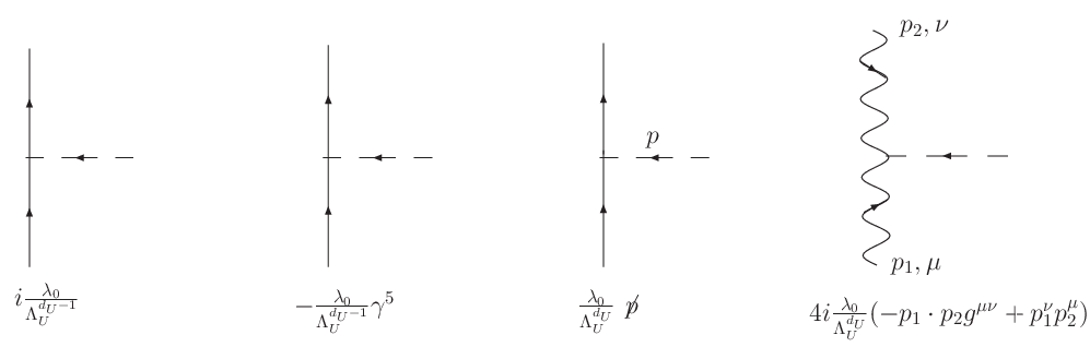
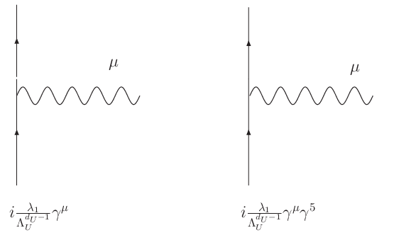
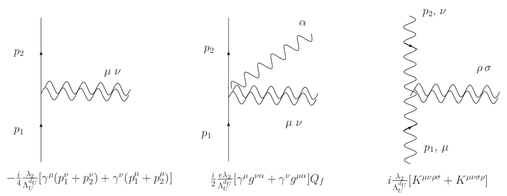
where the covariant derivative $D_{\mu}=\partial_{\mu}+ig\frac{\tau^{a}}{2}W^{a}_{\mu}+ig^{\prime}\frac{Y}{2}B_{\mu}$, $G^{\alpha\beta}$ denotes the gauge field strength (gluon, photon and weak gauge bosons), $f$ stands for a standard model fermion, $\psi$ stands for a standard model fermion doublet or singlet, and $\lambda_{i}$ are dimensionless effective couplings $C_{O^{i}_{\cal U}}\Lambda_{\cal U}^{d_{\cal BZ}}/M_{\cal U}^{d_{\rm SM}+d_{\cal BZ}-4}$ with the index $i=0,1$ and $2$ labeling the scalar, vector and tensor unparticle operators, respectively. Here we label each coupling constant $\lambda_{i}\;(i=0,1,2)$ the same for various operators of each spin. In principle, they can be different and they are then distinguished by additional indices. For simplicity we will also assume universality that $\lambda_{i}$’s are flavor blind. The Feynman rules for the operators in Eqs. (28), (29), and (30) are shown in Figs. 1, 2, and 3, respectively. Conventional wisdom tells us that the scalar operator $O_{\cal U}$ coupled to fermion is suppressed by the fermion mass. As already studied in georgi1,georgi2,ours, some of the operators listed above can give rise to interesting phenomenology, including real emission of unparticle as well as effective 4-fermion contact interactions. Phenomenology of unparticles that couple to flavor changing neutral currents have also been studied in georgi1, Luo-Zhu, Chen-Geng, Aliev-Cornell-Gaur, Li-Wei, Lu-Wang-Wang, Choudhury-Ghosh-Mamta. More gauge invariant operators that couple the spin-0 and spin-1 unparticle operators to SM fields are listed in Chen-He.

Virtual exchange of unparticle corresponding to the vector operator $O_{\cal U}^{\mu}$ between two fermionic currents can result in the following 4-fermion interaction (Fig. 4a) ours

The 4-momentum flowing along the unparticle propagator is $P_{\cal U}\equiv(p_{1}-p_{2})$. The contribution from the longitudinal piece $P_{\cal U}^{\mu}P_{\cal U}^{\nu}/P_{\cal U}^{2}$ in Eq. (24) has been dropped for massless external fermions. The convention of the fractional exponent of a complex number is already given in Eq. (17). The $(-)$ sign in front of $P_{\cal U}^{2}$ of the unparticle propagator in Eq. (31) gives rise to a phase factor $\exp(-i\pi d_{\cal U})$ for time-like momentum $P_{\cal U}^{2}>0$, but not for space-like momentum $P_{\cal U}^{2}<0$. For example, in Drell-Yan production the virtual exchange of unparticle in the $s$-channel will have $P_{\cal U}^{2}$ taken as the $\hat{s}$ of the subprocess and therefore will contain a phase. The most important feature is that the high energy behavior of the amplitude scales as $(\hat{s}/\Lambda_{\cal U}^{2})^{d_{\cal U}-1}$. For $d_{\cal U}=1$ the tree amplitude behaves like that of a massless photon exchange, while for $d_{\cal U}=2$ the amplitude reduces to the conventional 4-fermion interaction Eichten,contact, i.e., its high-energy behavior scales like $s/\Lambda_{\cal U}^{2}$. If $d_{\cal U}$ is between 1 and 2, say $3/2$, the amplitude has the unusual behavior of $\sqrt{\hat{s}}/\Lambda_{\cal U}$ at high energy. If $d_{\cal U}=3$ the amplitude’s high energy behavior becomes $(\hat{s}/\Lambda_{\cal U}^{2})^{2}$, which resembles the exchange of Kaluza-Klein tower of gravitons km. In principle, we can allow different couplings in different chirality combinations in the 4-fermion contact interactions, denoted by $LL,RR,LR,RL$, which can produce parity violation and therefore the forward-backward asymmetries. The combination of $LL+RR+LR+RL$ gives $VV$ interaction while $LL+RR-LR-RL$ gives $AA$ interaction that correspond to the vector and axial-vector interactions introduced in Ref. georgi2.

One can also consider the exchange of spin-2 unparticle between a pair of fermionic currents. The operator is given in Eq. (30) and the Feynman rule in Fig. 3. After simplification we arrive at the following 4-fermion interaction

for massless external fermions, where $p_{i}$ denotes the 4-momentum of the fermion $f_{i}$ along the fermion line (Fig. 4b). Note that the 4-fermion interaction induced by the spin-2 unparticle operator is further suppressed by $(s/\Lambda_{\cal U})^{2}$ relative to that induced by spin-1 unparticle operator. This is similar to the exchange by a spin-2 graviton (which corresponds exactly when $d_{\cal U}$ is set to 2 in Eq. (32).) Similarly, different chirality combinations are possible for the 4-fermion contact interactions with spin-2 unparticle exchange.

The above 4-fermion amplitudes can interfere with the standard model amplitudes of $\gamma$, $W$ and $Z$ exchange, and thus leads to interesting interference effects. In particular, the different spin structures could be differentiated by studying various angular distributions. Based on these spin-1 and spin-2 unparticle exchange amplitudes one can study the Drell-Yan process at hadron colliders, deep-inelastic scattering at $ep$ colliders, fermion pair production at $e^{-}e^{+}$ colliders, atomic parity violation, as well as many other low-energy $eq$ scattering processes, just in similar ways as the conventional 4-fermion contact interactions contact or as the Kaluza-Klein states of graviton km2. Modification of the Newton’s inverse square law in the sub-millimeter range due to spin-2 unparticle exchange and its possible tests at low energy gravity experiments have been studied in ungravity.

The close similarity between the unparticle and Kaluza-Klein (KK) modes of the large extra dimensions Arkani-Hamed:1998rs (LED) has been recognized ours in the calculation of the production cross sections and in virtual effects. The unparticle and the KK states Han:1998sg,Giudice:1998ck share analogous phase space integrations km, in particular the integration over the invariant mass squared $P^{2}$. It would be interesting to relate the unparticle with the KK modes in LED.

Let us first set up all fields of the standard model to be confined on a flat 3 dimensional spatial brane with coordinates $\bf x$. A scalar unparticle field can be identified as a massless scalar bulk field $\Phi(t,{\bf x},y)$ permeating into the LED described by extra coordinates $y_{i}$ $(i=1,\cdots,n)$. We study the simplest case that the space of LED is flat and periodic in each $y_{i}$ with periodicity $L$. The massless energy-momentum relation is

where ${\bf p}$ is the momentum in the ordinary 3-space and $k_{i}$ is the momentum component in LED. Periodic conditions on the extra dimensions require all the momenta $k_{i}$ to be quantized such that they are integral multiples of $2\pi/L$. As SM physics only operates on the 3-brane, the term $\sum_{i=1}^{n}(k_{i})^{2}$ of the corresponding KK modes effectively becomes the mass-squared of a particle propagating in the 3+1 spacetime. For large $L$, the summation over the KK modes turns into an integral and the density of states is introduced as

Identifying the power of $m^{2}$ in the density of states with the power of $P^{2}$ in the spectral density of the unparticle, we obtain

With one extra dimension we can have the notion of one-and-a-half particle viewed from the 3-brane, and so on. It is also tempting to make the following identification

with $d_{\cal U}$ given by Eq.(35). Perhaps hidden higher dimension spacetime reveals itself through the unparticle physics. It might be interesting to see if realistic models can be built based on this alternative interpretation of unparticle. Recently, it has been demonstrated in Stephanov that other values of $d_{\cal U}$ related to a dimensionless mass parameter can be achieved by deconstructing the unparticle in the 5 dimensional warped anti-de Sitter space using the AdS/CFT correspondence.

The energy spectrum of the mono-photon from the process $e^{-}(p_{1})\;e^{+}(p_{2})\;\to\gamma(k_{1})\;{\cal U}(P_{\cal U})$ can be used to probe the unparticle ours. Similarly, the mono-$Z$ production is also sensitive to the presence of some unknown particles or unparticle. Let us first derive the cross section formulas for mono-$Z$ production.

The differential cross section for $f(p)\,\bar{f}(p^{\prime})\to Z(k)\,{\cal U}(P_{\cal U})$ is given by

where $|\overline{{\cal M}}|^{2}$ is the spin- and color-averaged matrix element squared. Note that the invariant mass squared $P^{2}_{\cal U}$ of the unparticle is not fixed but is related to the energy $E_{Z}$ of the $Z$ boson via the recoil mass relation,

where the energy range of $E_{Z}$ is

As usual, we define $s=(p+p^{\prime})^{2}$, $t=(p-k)^{2}$ and $u=(p-P_{\cal U})^{2}$. Moreover, $s+t+u=M_{Z}^{2}+P_{\cal U}^{2}$.

As $d_{\cal U}$ approaches unity, we recover the on-mass-shell condition in the phase space

Thus, the integral over $E_{Z}$ is trivial and the cross section becomes

This reproduces the usual formula for $2\to 2$ cross section. This is expected since $d_{\cal U}\to 1$ corresponds to unparticle $\to$ particle. In this case, the energy spectrum for the $Z$ boson is just a delta function localized at $E_{Z}=E_{Z}^{\rm max}$.

References

- (1) S. Coleman and E. Weinberg, Phys. Rev. D7, 1888 (1973).
- (2) H. Georgi, Phys. Rev. Lett. 98:221601 (2007) [arXiv:hep-ph/0703260].
- (3) T. Banks and A. Zaks, Nucl. Phys. B196, 189 (1982).
- (4) H. Georgi, arXiv:0704.2457 [hep-ph]. (To appear in Phys. Lett. B)
- (5) K. Cheung, W. Y. Keung and T. C. Yuan, arXiv:0704.2588 [hep-ph]. (To appear in Phys. Rev. Lett.)
- (6) M.-x. Luo and G.-h. Zhu, arXiv:0704.3532 [hep-ph].
- (7) C.-H. Chen and C.-Q. Geng, arXiv:0705.0689 [hep-ph]; arXiv:0706.0850 [hep-ph].
- (8) G.-J. Ding and M.-L. Yan, arXiv:0705.0794 [hep-ph]; arXiv:0706.0325 [hep-ph].
- (9) Y. Liao, arXiv:0705.0837 [hep-ph].
- (10) T. M. Aliev, A. S. Cornell and N. Gaur, arXiv:0705.1326 [hep-ph]; arXiv:0705.4542 [hep-ph].
- (11) X.-Q. Li and Z.-T. Wei, arXiv:0705.1821 [hep-ph].
- (12) C.-D. Lu, W. Wang and Y.-M, Wang, arXiv:0705.2909 [hep-ph].
- (13) P. J. Fox, A. Rajaraman and Y. Shirman arXiv:0705.3092 [hep-ph].
- (14) N. Greiner, arXiv:0705.3518 [hep-ph].
- (15) H. Davoudiasl, arXiv:0705.3636 [hep-ph].
- (16) D. Choudhury, D. K. Ghosh and Mamta, arXiv:0705.3637 [hep-ph].
- (17) S.-L. Chen and X.-G. He, arXiv:0705.3946 [hep-ph]; S.-L. Chen, X.-G. He and H. C. Tsai, work in progress.
- (18) P. Mathews and V. Ravindran, arXiv:0705.4599 [hep-ph].
- (19) S. Zhou, arXiv:0706.0302 [hep-ph].
- (20) Y. Liao and J.-Y. Liu, arXiv:0706.1284 [hep-ph].
- (21) R. Foadi, M. T. Frandsen, T. A. Ryttov and F. Sannino, arXiv:0706.1696 [hep-ph].
- (22) M. Bander, J. L. Feng, A. Rajaraman and Y. Shirman arXiv:0706.2677 [hep-ph].
- (23) T. G. Rizzo, arXiv:0706.3025 [hep-ph].
- (24) H. Goldberg and P. Nath, arXiv:0706.3898 [hep-ph].
- (25) G. Mack, Commun. Math. Phys. 55, 1 (1977).
- (26) E. Eichten, K. D. Lane and M. E. Peskin, Phys. Rev. Lett. 50, 811 (1983).
- (27) V. D. Barger, K. m. Cheung, K. Hagiwara and D. Zeppenfeld, Phys. Rev. D 57, 391 (1998) [arXiv:hep-ph/9707412].
- (28) K. Cheung, arXiv:hep-ph/0409028.
- (29) K. Cheung, Phys. Lett. B 460, 383 (1999) [arXiv:hep-ph/9904510].
- (30) N. Arkani-Hamed, S. Dimopoulos and G. R. Dvali, Phys. Lett. B 429, 263 (1998) [arXiv:hep-ph/9803315].
- (31) T. Han, J. D. Lykken and R. J. Zhang, Phys. Rev. D 59, 105006 (1999) [arXiv:hep-ph/9811350].
- (32) G. F. Giudice, R. Rattazzi and J. D. Wells, Nucl. Phys. B 544, 3 (1999) [arXiv:hep-ph/9811291].
- (33) M. A. Stephanov, arXiv:0705.3049 [hep-ph].
- (34) K. m. Cheung and W. Y. Keung, Phys. Rev. D 60, 112003 (1999) [arXiv:hep-ph/9903294].
- (35) K. m. Cheung, W. Y. Keung and T. C. Yuan, Phys. Rev. Lett. 76, 877 (1996); S. Fleming, Phys. Rev. D 50, 5808 (1994); K. Hagiwara, A. D. Martin and W. J. Stirling, Phys. Lett. B 267, 527 (1991).
- (36) A. Heister et al. [ALEPH Collaboration], Eur. Phys. J. C 28, 1 (2003); J. Abdallah et al. [DELPHI Collaboration], Eur. Phys. J. C 38, 395 (2005) [arXiv:hep-ex/0406019]; P. Achard et al. [L3 Collaboration], Phys. Lett. B 587, 16 (2004) [arXiv:hep-ex/0402002]; G. Abbiendi et al. [OPAL Collaboration], Eur. Phys. J. C 18, 253 (2000) [arXiv:hep-ex/0005002].
- (37) K. m. Cheung, Phys. Lett. B 517, 167 (2001) [arXiv:hep-ph/0106251].
- (38) Particle Data Group, Review of Particle Physics, J. Phys. G: Nucl. Part. Phys. 33, 1 (2006).